Abstract
The rising popularity of machine learning has resulted in quality data becoming increasingly valuable. However, in some cases, the data are too sparse to effectively train an algorithm or the data cannot be disclosed to unaffiliated researchers due to privacy concerns. The sparsity of data may also affect various data analyses that require a certain volume of data to be accurate. One possible solution to the aforementioned problems is data generation. However, to be a viable solution, data generation must simulate real-life data well. To this end, this paper tests whether a previously presented iterative data generation method that generates synthetic data sets based on the attribute distributions and correlations of a real-life data set can faithfully reproduce a clustered data set. The approach is shown to be ineffective for the proposed application, and consequently, a new method is introduced that might preserve the clusters present in the real-life data set. The new method is demonstrated to not only preserve the clusters within the synthetic data set, but also improve the similarity of the attribute correlations of the synthetic data set and the real-life data set.
1. Introduction
Synthetic data are often utilized to thoroughly test and evaluate the robustness of a model or solution. The tests could require, for example, incorporating numerous edge cases, utilizing large volumes of data, testing with data that fulfill certain criteria, etc. When testing solutions, the focus is often on robustness—if a method is proved to be robust, it is deemed to be accurate enough. However, the similarity of the synthetic data to the real-life data can easily be overlooked. Any solution that will, once deployed, process real-life data should be tested with synthetic data that are as similar as possible in volume, type, and relationships to those the solution will ultimately be processing. Generating quality synthetic data is not a simple task for multiple reasons, such as privacy concerns [1], data sparsity, or data volume. However, if researchers can obtain an amount of real-life data relevant for their model, these data should be used to generate synthetic data sets that are large enough for testing.
Synthetic data prove especially useful when any kind of model is being developed with identifying data. Since synthetic data can retain valuable features without sacrificing privacy [2], they can enable other experts that do not have direct access to a real-life data set to analyze patterns and provide solutions without endangering the privacy of those whose data the data set contains [3]. Synthetic data are especially valuable in healthcare [4] and finance [5]. However, both fields require data of high quality to create models that are of high quality.
Two important questions arise when the goal is generating quality synthetic data that reproduce any of the characteristics of a real-life data set being used as a starting point:
- Which parameters are needed to generate a quality synthetic data set that reproduces the features of the real-life data set?
- How can the quality of a synthetic data set be measured or even determined?
Neither of the questions have a definite answer. The answer to the first question depends on either the researchers who are generating the synthetic data set or those who are providing the parameters for data generation. A perfect reproduction of the real-life data set may not only lead to data duplication, since the synthetic data set would be the same as the real-life data set, but also privacy concerns, which is why a level of variation in the generated data is welcome. This variation simulates naturally occurring variation present in real-life data. Each additional parameter that defines the features that should be reproduced in the synthetic data could lead to overfitting, which is why a precise number of parameters cannot be defined outright. Similarly, the quality of a synthetic data set is dependent on the task the data set will be used for. Nonetheless, if the inter-attribute correlations or attribute distributions of a real-life data set are not reproduced in a synthetic data set, the synthetic data cannot be considered a good substitute for the real-life data and should not be used as such. This reasoning led to interest in the Ruscio–Kaczetow method [6], which reproduces the aforementioned measures well. The method also reproduces non-normal distributions, an important aspect when simulating real-life data, since they are often not distributed normally. However, the method directly generates a synthetic data set from real-life data, an unsuitable characteristic when working with real-life data sets that are not open to the public or that have sparse anomalies. Therefore, a modification enabling synthetic data generation based on inter-attribute correlations and attribute distributions was proposed in [7], wherein the authors show those parameters are enough to generate a synthetic data set that reproduces inter-attribute correlations and attribute distributions well.
Another important aspect that should be reproduced in synthetic data are the clusters or classes present in a real-life data set (if the data set contains clusters or classes), which is why this paper expands on previous research by exploring how clusters can be maintained within the synthetic data. The method described in [7] is thoroughly tested alongside a further modified approach that should reproduce clusters. Additional measures and evaluations on downstream tasks are also provided to ensure the synthetic data are similar to real-life data. It is shown that the method described in this paper reproduces clusters in synthetic data, unlike the method described in previous research.
This paper is organized as follows: Section 2 defines the terms frequently used in the paper and provides related work; Section 3 describes the method presented in this paper; Section 4 describes the data set used as the basis for data generation; Section 5 shows the results of the conducted tests; Section 6 analyzes the results; and Section 7 concludes the paper and describes future work.
2. Basic Term Definitions and Related Work
Terms coined for or frequently used in this paper are defined or clarified in the next subsection. The definitions are followed by an overview of various researched data generation methods, with a focus on modern, deep-learning-based generative methods. The methods preceding the method presented in this paper are also examined.
2.1. Basic Term Definitions and Explanations
The term real-life data (or real-life data set) is used to denote data that can be observed, measured, or obtained from real-world sources or events. They are the opposite of the data in a synthetic data set; a data set constructed by an algorithm or a method that can create data. The terms generated synthetic data set and generated data set are also used for the aforementioned definition. A starting data set is the input required for a data generation method that creates data according to the characteristics of another data set (real-life or synthetic). Furthermore, the method that produces a synthetic data set is called a synthetic data generator or simply a data generator.
Please note that cluster and class are used interchangeably in this paper due to the nature of the real-life data set used for data generation. One class corresponds to one cluster in the example data set.
2.2. Different Approaches to Data Generation
The way synthetic data are generated varies depending on the downstream task they are generated for. In some cases, the characteristics of the data are less relevant than the number of data points, whereas in other cases reproducing the characteristics of real-life data is the main goal. Therefore, various algorithms and methods were reviewed to gain an overview of the field and further insight into the goals and challenges of data generation. The approaches were grouped according to apparent similarities. The following is a list of simplified data generation categories observed during research:
- Methods that use a small sample or a small starting data set, the contents of which they replicate and add a certain amount of noise to [8,9];
- Methods that input the starting data set into a simpler machine learning algorithm and train it, then extract elements of the trained solution to use for synthetic data generation [10,11,12,13,14];
- Methods that leverage the capabilities of deep learning solutions to learn the characteristics of real-life data for tabular data synthesis, such as Generative Adversarial Networks (GANs) [15,16,17,18,19,20,21,22,23], Variational AutoEncoders (VAEs) [24,25,26,27], and Large Language Models (LLMs) [28,29,30,31];
- Methods that rely on lists of values extracted from relevant (starting) data sets, where each attribute value of a synthetic data set is sampled from a corresponding value list [32,33,34,35,36,37,38,39,40,41,42];
- Methods that use characteristics obtained from a starting data set to generate synthetic data [6,43,44,45].
In recent years, deep learning solutions have gained popularity due to the accessibility of generative models. Transfer learning and the possibility of fine-tuning existing models to specific tasks have also aided the adoption of such architectures. However, the variety of data and downstream tasks the data will be used for leads to great variety in the field [46]. Generalization is still an active problem due to the characteristics of the algorithms. In particular, deep learning solutions are prone to overfitting, mainly when their training sample is small [47], which is a possibility when using real-life data. In such cases, deep learning solutions are often outperformed by classic statistical methods [48]. Furthermore, they often require substantially more resources to achieve quality results, both when considering the size of the starting data set and the necessary processing power, especially when using an LLM [49] (such as in [28]). Another LLM specific issue is their susceptibility to hallucinations [50,51], which could greatly impact the quality of the synthetic data. GAN-based solutions can have issues reproducing the distributions of the original data set [25], as well as being particularly susceptible to model collapse [49]. Moreover, due to the adversarial nature of the training process, GAN models require careful hyperparameter tuning to achieve stable convergence [52]. Synthetic data generators based on VAEs often produce data that are too similar to the data from the original data set, often reducing overall synthetic data quality [25,49]. Therefore, machine learning solutions are frequently made to solve a particular problem or generate a particular type of data set based on examples. In those cases when the examples are of real-life data, their tendency to overfit can lead to privacy concerns [53,54]. Also, explainability in deep learning is still lacking [55], especially in LLMs, a characteristic that could lead to further risks when generating synthetic data [56]. However, requiring real-life data is not unique to machine learning solutions; in the aforementioned list, only the last category can generate data without direct access to a starting (real-life) data set.
The aforementioned overview and working with personal data led the authors to explore methods from Category 5 in [7]. In this work, the authors used summary data (inter-attribute correlations and attribute distributions) to test generating quality synthetic inter-user relationship data based on real-life Facebook relationships. The authors showed that the method presented in [6] can be modified to generate data without using a real-life data set. This modification is necessary due to the original method resampling the real-life data set to form the basis of the synthetic data set. The modification of the method described in [7] uses the quantiles of each of the attributes of the starting data set, creating new data points by interpolating the quantiles. After analyzing the synthetic data sets generated by the modified approach, it was concluded the approach was a viable way of generating synthetic data without a direct need for a real-life data set.
The following subsection describes the original method presented in [6], and the steps needed to develop the modified method from [7]. The two approaches are the basis of the method proposed in this paper.
2.2.1. Ruscio–Kaczetow Method
The Ruscio–Kaczetow method (or the original method) is the method first proposed by Ruscio and Kaczetow in [6]. This method is a slight modification of the approach proposed by Ruscio et al. in [57]. The input of the Ruscio–Kaczetow method is a data set whose correlation matrix is calculated and whose data points are first sampled with repetition per each attribute. The sampled data points are the basis of the synthetic data set and there are as many of them as there are data points in the starting data set. After the sampling, the method instantiates three matrices: two are populated with normal values, and the third matrix temporarily stores the result of each iteration of the method. The matrices enable switching from calculation with normal values to calculation with non-normal values. The two random value matrices and the correlation matrix of the data set are used to calculate a weighted normal value for each sampled data point. The calculated values are saved into a placeholder matrix, then sorted and replaced with values from the sample data set. The correlation matrix of the resulting data set is calculated and compared to the correlation matrix of the starting data set. The comparison is based on the following formula:
where denotes the elements under the main diagonal from the difference of the correlation matrix of the resulting data set and the correlation matrix of the starting data set, and k is the number of attributes present in the starting data set. If the stopping criterion of the method is met (the value has not reduced for several iterations), the result of the calculation is the generated synthetic data set. The described steps have been written out in pseudocode form in Algorithm 1. Certain parts of the algorithm have been abstracted for easier viewing and understanding. A starting data set is the only requirement for generating synthetic data with this method.
For a clear and concise view of the steps necessary to generate synthetic data using the original Ruscio–Kaczetow method, a flowchart has been provided in Figure 1.
| Algorithm 1: Ruscio–Kaczetow data generation algorithm |
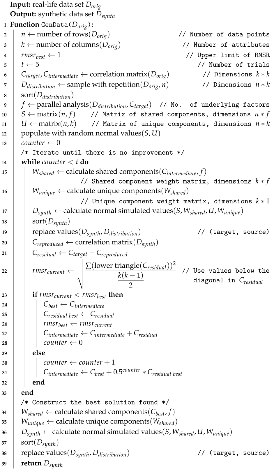 |
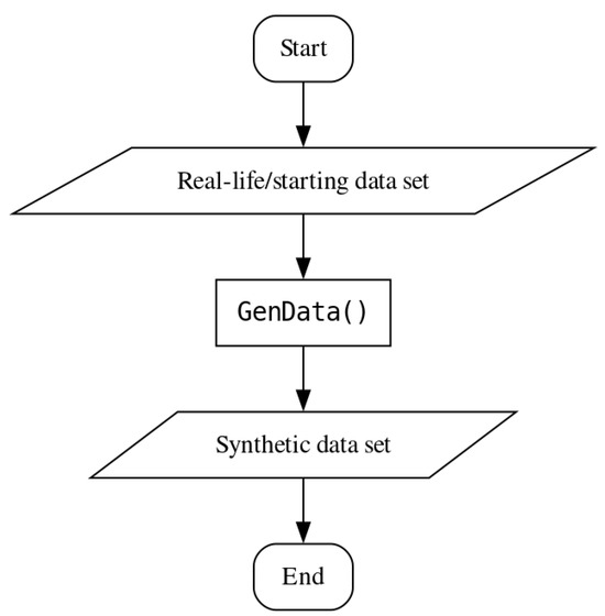
Figure 1.
Flowchart for using the original synthetic data generation method.
2.2.2. Modified Ruscio–Kaczetow Method
The modified method, first proposed in [7], adds elements to and changes parts of the previously described method. Namely, instead of generating a synthetic data set from the starting data set directly, the modified method requires the correlation matrix and the quantiles of each of the attributes of the starting data set as input. The attribute quantiles are interpolated very finely and used as the basis of the synthetic data set. A dilation factor is set to create a large data set of interpolated values, from which the desired number of data points is sampled. This change of approach enables generating synthetic data sets of desired size. The sampling to form the attribute distributions from the original method is eliminated and the sampled interpolated data points are used for all the calculations directly. The correlation matrix of the starting data set is also calculated in advance and used as part of the input. These modifications offer several benefits when compared to the original method:
- The method does not require a starting data set as direct input;
- The data points used for data set generation are calculated and, therefore, less likely to exist in the starting data set;
- There is no limit on the size of the data set the method can generate.
This method could allow researchers to work with data they cannot directly use due to privacy concerns since it does not require a starting data set as direct input. The synthetic data sets the modified method generates are more varied than those produced by the original method due to the use of calculated values instead of values sampled directly from the starting data set. The theoretically limitless size of the synthetic data sets should be useful when an application requires more data points than are originally available.
This paper uses the described modified method as a benchmark to illustrate the effects of the proposed further changes to the method. It will be referred to as the benchmark method further in text.
Algorithm 2 describes the method used to interpolate the quantiles of a starting data set. It incorporates the possibility of choosing how numerous the resulting interpolated data should be (variable n), as well as how much larger the data set they are sampled from should be (variable d).
| Algorithm 2: Data interpolation algorithm |
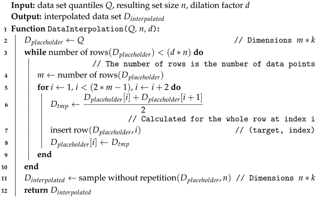 |
Algorithm 3 details the changes made to Algorithm 1 when switching from generating synthetic data directly from a real-life data set to generating the data from an interpolated data set. Only the lines that need to be changed in Algorithm 1 are included.
| Algorithm 3: Changes made to the Ruscio–Kaczetow algorithm |
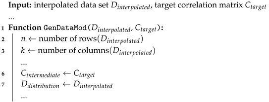 |
For a simple overview of the steps necessary for using the benchmark method, please refer to Figure 2. The steps below the dashed line do not require direct access to the starting data set, which enables external researchers to generate synthetic data based on attribute quantiles and inter-correlations.
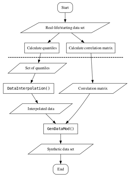
Figure 2.
Flowchart for using the benchmark synthetic data generation method.
3. Methodology
After extensively testing the benchmark method with the correlations and distributions of a data set describing user interactions on Facebook (the analysis of the data set is available in [58]; benchmark method testing in [7]), it was not clear whether class or cluster information remained within the synthetic data. A suitable data set with clear clusters was required for determining whether the information was still extant after data generation. The clear clusters are necessary both for human readability and for clear clustering results when determining the quality of the resulting synthetic data set. The freely available “texture” data set was chosen for testing due to having suitably distinct clusters. The data set was filtered for greater result clarity.
Firstly, the benchmark method was used to generate a synthetic equivalent of the filtered “texture” data set. Analyses indicated that no clusters present in the real-life data set were preserved in the synthetic data set, even though the distributions and correlations were. Therefore, additional changes were made to the already modified method (following some of the recommendations from [57]).
When using the proposed approach, referred to as the cluster preserving method in the following text, the starting data set needs to be split into subsets according to class. The inter-attribute quantiles and correlation matrices of each subset need to be calculated separately, as well as the proportion of the subset in the starting data set. The quantiles and proportions are used to interpolate and sample a desired number of points that serve as the basis for data generation. The interpolated data points are then paired with the correlation matrix of the originating subset and run through the modified data generation algorithm (Algorithm 3). The resulting generated subsets are combined into a single synthetic data set after data generation. This change in approach results in the following advantages when compared to the benchmark method:
- The method preserves class or cluster information in the synthetic data;
- The method maintains class or cluster proportions in the synthetic data.
The method even allows changing class proportions in the synthetic data set by providing different proportions during the interpolation step of data generation.
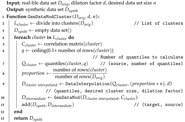
Algorithm 4 outlines the whole process of data generation with the cluster preserving method. The data generation starts with the real-life data set and the desired resulting synthetic data set size for clarity. However, the synthetic data set can be generated with a list of cluster quantiles, list of cluster correlation matrices, list of cluster proportions, a desired dilation factor, and the desired resulting synthetic data set size, entirely removing the need for directly using a real-life data set.
| Algorithm 4: Generating a synthetic data set with preserved clusters |
 |
To enable quick comparison between the three described methods, a flowchart for the cluster preserving method can be seen in Figure 3. As with Figure 2, all the elements drawn underneath the dashed line do not require direct access to the starting data set. Also, if the starting data set does not contain clusters or classes, synthetic data generation should follow the steps outlined in Figure 2, as indicated by the right branch of the conditional block in Figure 3.
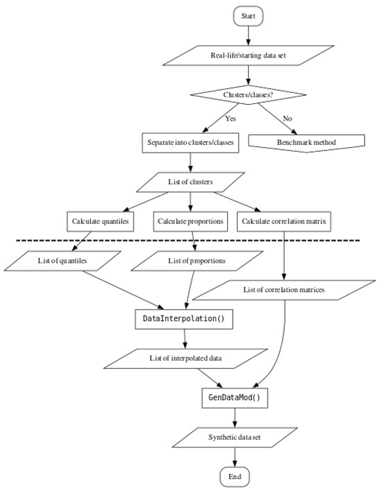
Figure 3.
Flowchart for using the cluster preserving synthetic data generation method.
The cluster preserving method was used to generate a synthetic equivalent of the filtered “texture” data set as well. The synthetic data set was analyzed to determine whether the resulting distributions, correlations, and clusters were comparable to the correlations, distributions, and clusters of the real-life data set, as well as whether the resulting synthetic data set approximated the real-life data set more closely than the synthetic data set generated by the benchmark method.
Implementation and Comparisons
Algorithm 4 was implemented in the programming language R (“a free software environment for statistical computing and graphics”, https://www.r-project.org/, version 4.4.2), as were the previous versions. The flowcharts were created with the Graphviz software (“open source graph visualization software”, https://graphviz.org/, version 12.1.0).
The quality of the generated synthetic data sets was determined through multiple analyses. The quantiles of the synthetic data sets were calculated and compared to the quantiles of the starting data set. The differences between the correlation matrices of the synthetic data sets and the correlation matrix of the starting data set were visualized. Statistical tests were used to determine the similarity of the synthetic data and the real-life data. The package “twosamples” (“Fast randomization based two sample tests.”, https://cran.r-project.org/web/packages/twosamples/twosamples.pdf, accessed on 23 April 2025) was chosen due to enabling the comparison of two data samples with a different number of data points. The two statistical methods chosen from the package were “DTS” [59] and the Anderson–Darling statistical test [60]. The tests were used to test the hypothesis that two samples come from the same distribution with an alpha value of . Finally, the synthetic data sets were evaluated on a downstream task.
4. Data Set
The data set “texture” was used for data generation. The primary characteristics of the data set are: a sizable number of attributes (40), no missing values, numerous instances per class (500; overall 5500 instances), and clearly labeled classes (11; each corresponds to a real-life texture). It is also a real-life data set, which makes it suitable for data generation in the context of this paper. A spatial distribution of the data set can be seen in Figure 4 in three dimensions. The class labels can be seen on the right-hand side of the figure. Attributes ‘V10’, ‘V23’, and ‘V30’ (labeled as ‘A10’, ‘A23’, and ‘A30’ in the data set file) are used as the x-, y-, and z-axes, respectively.
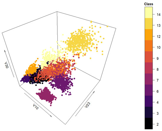
Figure 4.
Three-dimensional view of the “texture” data set.
In order to make the preliminary results more human-readable and interpretable, 6 of the 40 attributes and 4 of the 11 classes were chosen for data generation—attributes ‘A10’, ‘A19’, ‘A23’, ‘A25’, ‘A30’, and ‘A35’ (renamed ‘V10’, ‘V19’, ‘V23’, ‘V25’, ‘V30’, and ‘V35’ in this paper) and classes ‘6’, ‘7’, ‘12’, and ‘13’. The chosen attributes provide the most distance between the classes, and the chosen classes are spatially far apart. Both characteristics enable visual analysis by humans. The filtered data set has 2000 instances. The spatial relationship of the filtered data set can be seen in Figure 5 in three dimensions.
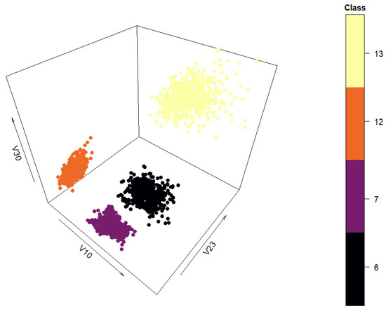
Figure 5.
Three-dimensional view of the classes selected from the “texture” data set.
A second data set, the “yeast” data set, was also used to evaluate the proposed method. The description of the data set, the results of data generation, and their analysis can be found in Appendix A.
5. Results
Firstly, the entire filtered data set was used as the input for the benchmark method—201 quantiles were calculated for each of the attributes of the data set and the correlation matrix of the data set was calculated, after which both were used to generate a synthetic data set. The resulting data set can be seen in Figure 6.
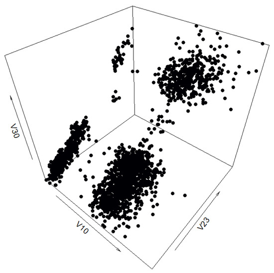
Figure 6.
Three-dimensional view of the synthetic “texture” data set generated by the benchmark method without prior cluster separation for data interpolation.
However, after plotting the synthetic data set generated without any prior separation according to cluster, it was decided comparing synthetic data sets generated by the benchmark method and the cluster preserving method using the same interpolated data points would yield clearer and more mathematically sound results. Since the interpolation step can be separated from the generation step, the data points can be interpolated cluster by cluster, but then treated as a singular data set that can be used by the benchmark method (please note this paper compares the benchmark method and the cluster preserving method using the same data points obtained by interpolating cluster by cluster, unless otherwise stated). Therefore, 51 quantiles were calculated for each of the clusters chosen when filtering the data set, as were correlation matrices (both for the whole data set, to be used by the benchmark method, and one for each cluster, to be used by the cluster preserving method). The quantiles were then interpolated cluster by cluster. After this step, two synthetic data sets were generated from the same data points: one was generated by combining all the interpolated data points and using them and the calculated correlation matrix of the filtered real-life data set as the input for the benchmark method, whereas the other was generated by using the sets of data points interpolated from cluster quantiles and the corresponding correlation matrices as input for the cluster preserving method.
The synthetic data set generated by the benchmark method has 2000 data points and can be seen in Figure 7. Figure 8 is a comparison plot of the quantiles calculated from the real-life data set and the ones calculated from the synthetic data set. Figure 9 is the residual correlation matrix, which is the result of the following calculation:
where denotes the matrix of correlation residuals, the correlation matrix of the starting data set and the correlation matrix of the synthetic data set. The Anderson–Darling and DTS statistical tests were also used to determine the similarity of the attributes of the real-life data set and the synthetic one. The p-values obtained from the tests can be observed in Table 1.
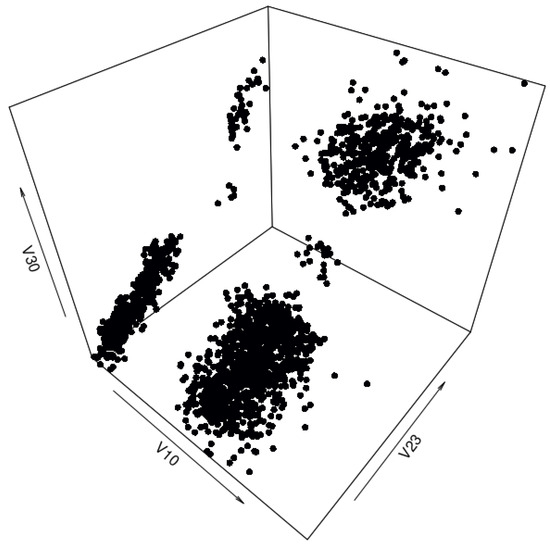
Figure 7.
Three-dimensional view of the synthetic “texture” data set generated by the benchmark method with prior cluster separation for data interpolation.
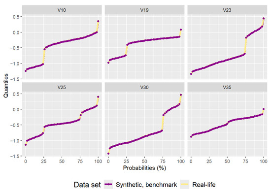
Figure 8.
Plot of quantiles calculated for the real-life data set and the synthetic data set generated by the benchmark method.
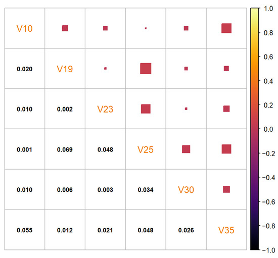
Figure 9.
Residual correlation matrix of the synthetic “texture” data set generated by the benchmark method.

Table 1.
Table of p-values calculated by the Anderson–Darling and DTS statistical tests comparing the distributions of the attributes of the filtered data set and the attributes of the synthetic data set generated by the benchmark method.
The synthetic data set generated by the cluster preserving method also has 2000 data points, with 500 data points being generated per each cluster (to correspond to the real-life data set). After generation, the individual cluster data sets were combined into a single synthetic data set that can be seen in Figure 10. A quantile comparison graph (Figure 11) and a residual correlation graph (Figure 12) were also plotted for this synthetic data set. Please note that the residual correlation matrix was plotted for the combined data set. The matrix was calculated using (2). The results of the statistical tests can be seen in Table 2.
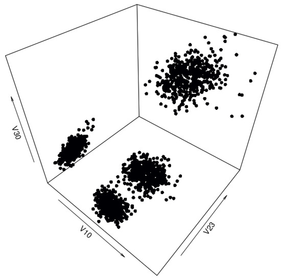
Figure 10.
Three-dimensional view of the synthetic “texture” data set generated by the cluster preserving method.
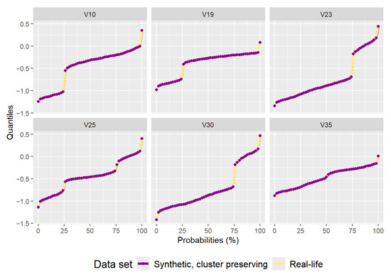
Figure 11.
Plot of quantiles calculated for the real-life data set and the synthetic data set generated by the cluster preserving method.
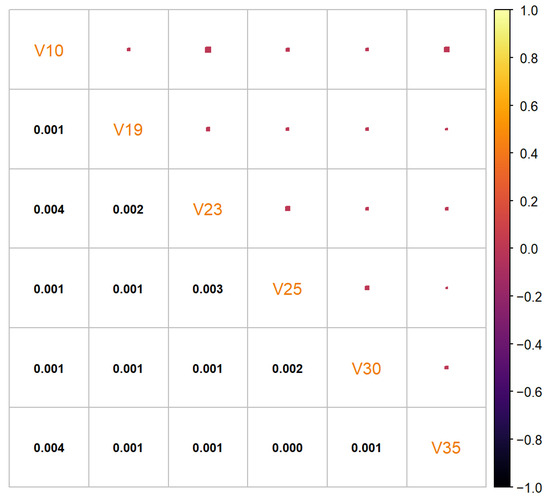
Figure 12.
Residual correlation matrix of the synthetic “texture” data set generated by the cluster preserving method.
Table 2.
Table of p-values calculated by the Anderson–Darling and DTS statistical tests comparing the distributions of the attributes of the filtered data set and the attributes of the synthetic data set generated by the cluster preserving method.
For a final comparison between the real-life data set, data set generated by the benchmark method, and data set generated by the cluster preserving method, the densities of each of the attributes were calculated and plotted on the same graph, as can be seen in Figure 13. The three densities overlap almost completely, an expected outcome that highlights the importance of choosing the right synthetic data set quality measures, an issue further discussed in detail in Section 6.
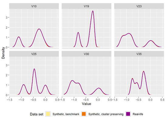
Figure 13.
Comparison of the densities of the attributes of the real-life data set and the attributes of the synthetic data sets (one generated by the benchmark method, the other generated by the cluster preserving method).
Since the clusters in the synthetic data set generated by the benchmark method are not comparable with the ones present in the real-life data set, statistical tests calculated for each set of values an attribute takes for each of the distinct classes (and therefore, clusters) were calculated for the real-life data set and the synthetic data set with the preserved clusters. The results can be seen in Table 3.
Table 3.
Table of p-values calculated by the Anderson–Darling and DTS statistical tests comparing the distributions of each of the attributes (“Attr.” in table) of the filtered data set and the synthetic data set (cluster preserving method) depending on the class (“Cls.” in table).
Multiple views of the filtered real-life data set, synthetic data set produced by the benchmark method, and the synthetic data set produced by the cluster preserving method can be found in Appendix B.
Downstream Task—Clustering
To test the hypothesis that the synthetic data generated by the cluster preserving method can be used for tasks that real-life data would otherwise be necessary for, both the real-life data set and the generated synthetic data set were subjected to clustering. Both were clustered using the k-means clustering method (the built-in kmeans function of the R programming language was used). Since both data sets retain the information which cluster the data points belong to, one random data point from each cluster was used as the initial center for each cluster. The results of the clustering can be seen in Figure 14. Each of the clusters in both cases has 500 data points.
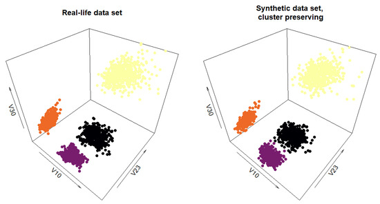
Figure 14.
Plot of the clustering results for the real-life data set and the synthetic data set generated by the cluster preserving method.
The centroids of each of the clusters identified in the data sets were calculated as well and can be seen in Table 4.
Table 4.
Calculated coordinates per attribute ("Attr." in table) for (“Cnt.” in table) for both the real-life data set and the synthetic data set generated by the cluster preserving method, in tabular form.
The within-cluster sum of squares can be seen in Table 5.
Table 5.
Within-cluster sums of squares for both the real-life data set and the synthetic data set generated by the cluster preserving method, in tabular form.
6. Discussion
Comparing Figure 5, Figure 6 and Figure 7 leads to a clear conclusion that generating a synthetic data set using the benchmark method does not retain the spatial distribution of the data set used for generation. However, the following images, namely Figure 8 and Figure 9, indicate that the quantiles and correlation matrix of the synthetic data set are still similar to those of the real-life data set. Table 1 also corroborates the possibility of the synthetic data set being a good reproduction of the real-life data set. The results of the various tests, both visual and statistical, show the importance of choosing a humanly legible data set for initial tests. Without the clear visual comparison, the results could have been considered good enough, and an important aspect of the real-life data set would have been lost.
The synthetic data set generated by the cluster preserving method is visually similar to the real-life data set, unlike the synthetic data set generated by the benchmark method. A visual comparison of Figure 5, Figure 7, and Figure 10 leads to the conclusion that the starting data set should be separated into clusters (when it is a data set with clusters). It is important to note that the quantiles visible in Figure 11 are the quantiles for the full synthetic data set; therefore, even though the quantiles used to generate each of the clusters were exclusively the quantiles of that cluster, the full synthetic data set retains attribute distributions overall with minimal variation. Furthermore, since both of the synthetic data sets were generated from the same data points, the quantiles for each of the attributes are essentially the same. Therefore, even though the quantiles of the synthetic data sets are very similar to the quantiles of the real-life data set, they cannot help identify whether there is a difference in synthetic data set quality between the two data generation methods. However, the residual correlation matrices indicate a difference. A visual comparison of Figure 9 and Figure 12 determines that splitting the starting data set by cluster when generating a synthetic data set results in the correlation matrix of the synthetic data set more closely matching the correlation matrix of the starting data set. When comparing the two numerically, the residual correlation matrix of the synthetic data set generated using the benchmark method has a sum of residuals above the main diagonal of with an average residual of , whereas the residual correlation matrix of the synthetic data set generated using the cluster preserving method has a sum of above the main diagonal with an average residual of . Therefore, generating the synthetic data set cluster by cluster yields a reduction of correlation matrix residuals by at least an order of magnitude. Once again, even though the synthetic data set was generated with the correlation matrices of each of the clusters, the values of the correlation matrix of the full synthetic data set are almost equal to the values of the correlation matrix of the real-life data set.
The results of the statistical tests available in Table 1 and Table 2 once again do not conclusively show whether one of the synthetic data sets simulates the real-life data set more closely. Neither the Anderson–Darling test nor the DTS test give a clear indication which of the two synthetic data sets is of better quality. However, since both tests randomly resample the data sets they are calculated with, the differences between the observed p-values are likely due to the seed the two test functions are seeded within the R programming language. The hypothesis that the synthetic attributes of either of the synthetic data sets belong to the distribution of the attributes of the real-life data set cannot be rejected. It is important to note that, even though the Anderson–Darling statistical test is one of the most frequently used statistical tests in scientific literature, DTS likely has more stable properties when presented with various distributions [59]. Since the distributions of the real-life data set are distributions of real-life properties, they cannot be expected to conform to standard mathematical distributions, which could explain the lower p-values observed in the Anderson–Darling test results.
Additionally, Figure 13 confirms both the synthetic data generation and subsequent quality analyses of synthetic data sets need to be executed carefully. Using the same data points for both synthetic data sets ensures their densities overlap completely. Similarly, due to the interpolation step of the synthetic data generation methods, the densities of the synthetic attributes correspond to the densities of the real-life attributes.
Finally, the p-values comparing the real-life data set and the synthetic data set generated using the cluster preserving method, calculated for each of the attributes depending on the cluster the data belong to (Table 3), show that the hypothesis the two samples are part of the same distribution cannot be rejected. The difference between the two statistical tests is consistent with the trend of the results of the previous tests (Table 1 and Table 2), where the results of the Anderson–Darling test are poorer than the results of the DTS test. Even though each of the clusters of the synthetic data set was generated with the corresponding real-life cluster attributes, the overall distributions of the attributes are mathematically more similar than the distributions of the attributes within the clusters. It is possible this is due to the number of data points in each of the clusters.
The downstream task (Section 5) further corroborates the assessment that the synthetic data retain a significant number of the qualities of the real-life data set. The clusters were perfectly identified, the calculated centroid coordinates for both the real-life data set and the synthetic data set are very close in value, as are the within-cluster sums of squares.
The analyses indicate that the chosen number of quantiles calculated from the real-life data set (51 per cluster with four clusters, therefore 204—around 10% of the number of data points in the real-life data set) is enough to create a synthetic data set whose attribute distributions, correlations, and classes correspond to those of the real-life data set. Even though the attributes were separated by cluster, resulting in the interpolated data points being sampled from a segment of the real-life attribute distributions and the final synthetic clusters being generated with just the cluster correlation matrices, the overall measures conform to the measures of the real-life data set.
All the tests run on the three data sets also emphasize the importance of thoroughly analyzing the data set being used as the starting data set for synthetic data generation. The method described in this paper is not only suitable but necessary when generating a data set with clustered data. On the other hand, if the starting data set does not have clusters, it should be generated outright, without splitting into clusters. A synthetic data set that could be substituted for a real-life data set can only be generated from the characteristics of a well-studied data set. Furthermore, once the synthetic data set is generated, multiple characteristics of this data set should be compared to those of the real-life data set, especially if the final goal is to have a synthetic data set that could in fact be used for analyses instead of the real-life data set. This can only be performed by researchers that have direct access to the real-life data set.
7. Conclusions
This paper presents an adaptation of the synthetic data set generation method presented in [7] that ensures the preservation of clusters in the synthetic data it generates. The previously proposed method generates a synthetic data set based on the distributions of individual attributes as well as the inter-attribute correlations of a starting data set, and achieves significant overlap between those measures in the synthetic and starting data sets. However, it demonstrates limited effectiveness when applied to starting data sets that contain clusters. In such cases, although correlations and attribute distributions are retained, the clusters characteristic of the original data set are typically lost in the synthetic counterpart.
The method proposed in this paper addresses this deficiency by introducing an adaptation that preserves not only attribute distributions and inter-attribute correlations, but also the inherent clustering structure of the original data set.
An important advantage of the proposed cluster preserving method is that it enables the generation of data sets larger than the original, while maintaining the relative proportions of all classes present in the source data.
Additionally, an important feature of the proposed approach is also its ability to alleviate data scarcity, which is useful in contexts where machine learning algorithms require large quantities of data to effectively learn relevant patterns. Since the method produces previously unseen data points, it could also help mitigate overfitting in artificial neural networks and similar models.
Another notable benefit is the potential to facilitate greater data sharing. The method could allow organizations to generate synthetic data sets that obscure sensitive real-life data while retaining the analytical value of said data. This could enable external researchers to develop solutions based on these data sets without compromising privacy—an especially valuable feature in sensitive domains such as healthcare and finance.
It is also worth emphasizing that, unlike many deep-learning-based synthetic data generators, the method presented here is explainable.
Future study should investigate the assumptions related to machine learning and further assess how the proposed method could address common issues associated with such algorithms. Moreover, extending the method to support data sets with multiple nominal attributes beyond the class label represents a promising direction for future research. Such an enhancement would significantly broaden the range of data sets which this method could be applied to.
Author Contributions
Conceptualization, L.H., M.V. and L.P.; methodology, M.V., L.H. and L.P.; software, L.P.; validation, L.P., L.H. and M.V.; formal analysis, L.P., L.H. and M.V.; investigation, L.P., L.H. and M.V.; resources, M.V., L.H. and L.P.; writing—original draft preparation, L.P.; writing—review and editing, L.H., M.V. and L.P.; visualization, L.P. and L.H.; supervision, M.V. and L.H.; funding acquisition, M.V. and L.H. All authors have read and agreed to the published version of the manuscript.
Funding
This research has been supported by the European Regional Development Fund under the grant PK.1.1.10.0007 (DATACROSS).
Informed Consent Statement
Not applicable.
Data Availability Statement
The “texture” data set, used to test the hypotheses presented in this work, is freely available as part of the repository of the Knowledge Extraction based on Evolutionary Learning (KEEL) software tool at: https://sci2s.ugr.es/keel/dataset.php?cod=72 (accessed on 13 March 2025). Furthermore, the “yeast” data set, used to further test the hypotheses, is also freely available as part of the same repository at: https://sci2s.ugr.es/keel/dataset.php?cod=1063 (accessed on 21 April 2025).
Conflicts of Interest
The authors declare no conflicts of interest.
Abbreviations
The following abbreviations are used in this manuscript:
| GAN | Generative Adversarial Network |
| LLM | Large Language Model |
| RMSR | Root Mean Square Residual |
| SVM | Support Vector Machine |
| VAE | Variational AutoEncoder |
Appendix A. Analysis and Synthetic Data Generation for the “Yeast” Data Set
The “yeast” data set is an additional data set used to test the method described in this paper. The data set consists of 8 attributes, 1484 instances, and 10 classes the instances can belong to. There are no missing values in the data set. All the attributes are numerical in value. The number of instances per class is highly imbalanced, as can be seen in Table A1. As with the “texture” data set, the “yeast” data set is a real-life data set.
Table A1.
Number of instances per class in the “yeast” data set.
Table A1.
Number of instances per class in the “yeast” data set.
| Class | CYT | ERL | EXC | ME1 | ME2 | ME3 | MIT | NUC | POX | VAC |
| No. of instances | 463 | 5 | 35 | 44 | 51 | 163 | 244 | 429 | 20 | 30 |
The spatial distribution of the data set can be seen in Figure A1. Since the graph clearly indicates clustering would not be an appropriate downstream task for this data set, classification was chosen instead.
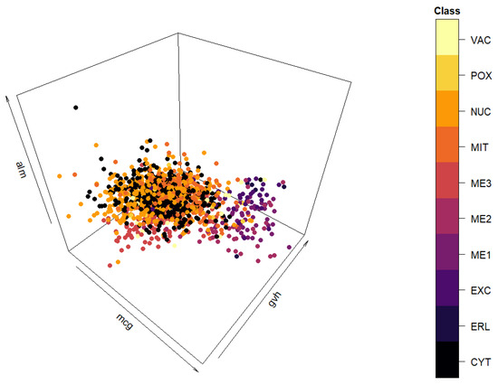
Figure A1.
Three-dimensional view of the “yeast” data set.
This data set posed two challenges when generating synthetic data. The first challenge was that the values of the attributes ‘erl’ and ‘pox’ have very little variation. When splitting the data into classes before data generation, some of the subsets had only one value of these attributes, which led to the occurrence of undefined values (denoted by the logical constant NA in the R programming language) when calculating the class correlation matrices. There is a simple solution that can be built into the synthetic data generation methods (either the benchmark method or the cluster preserving one) without losing any previous functionality or generality—the attributes with no variance are excluded from the data interpolation and data generation step. Once data generation has been carried out, the attributes are added back into the synthetic data set. The second challenge stems from the smallest cluster having only five instances. Namely, Algorithm 3 uses parallel analysis to determine the number of underlying factors in a starting data set (if the value is not explicitly stated when calling the function in a program). This entails creating an (number of instances * number of attributes) sized matrix and populating it with attribute instances sampled with replacement from the starting data set. This matrix is used to calculate a correlation matrix whose eigenvalues are then computed. The small size of the ‘ERL’ class makes the probability of sampling the same value for all the instances of an attribute fairly likely. This leads to a higher likelihood of NA values occurring in the correlation matrix. The solution to this challenge can also be built into the approaches without changing their prior behavior and generality—the matrix populated with randomly sampled values should be checked for value uniqueness. If the values of the instances of an attribute are all the same, the value sampling should be redone. The sampling should be repeated until there are no columns (attributes) with just one value. Once the two challenges have been solved, a synthetic “yeast” data set can be generated.
Synthetic data set generation closely followed the approach described in Section 3. The real-life data set was split by class. Quantiles, class proportions, and correlation matrices were calculated for each of the classes (the correlation matrix of the whole real-life data set was calculated for the benchmark method). The quantiles and the class proportions were used to create an interpolated data set for each of the classes. Those data and the corresponding correlation matrices were used to generate synthetic classes that were combined into a single data set (the interpolated data were also combined into one starting data set and used alongside the whole data set correlation matrix to generate a synthetic data set using the benchmark method).
The synthetic data set generated by the benchmark method can be seen in Figure A2. It has 1483 data points. Even though the data points are not of different colors, it is visible that the data do not follow the distribution of the real-life data set. The quantiles are almost perfectly replicated, as can be seen in Figure A3, as with the “texture” data set. The very low variance of the ‘erl’ and ‘pox’ attributes can clearly be seen in the quantiles. The residual correlation matrix can be seen in Figure A4. The sum of the residuals in the matrix above the main diagonal is and the average residual value is . The results of the statistical tests can be seen in Table A2. Due to the low variance of some of the attributes the statistical tests reject (Anderson–Darling) or almost reject (DTS) the hypothesis the synthetic data are from the same distribution as the real-life data set.
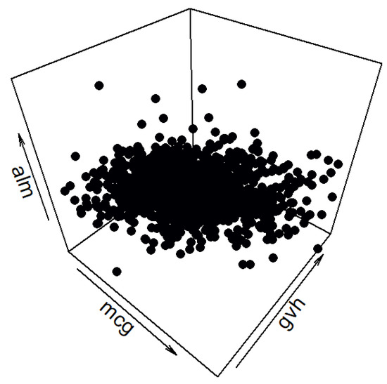
Figure A2.
Three-dimensional view of the synthetic “yeast” data set generated by the benchmark method.
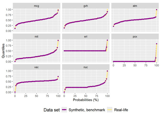
Figure A3.
Plot of quantiles calculated for the real-life “yeast” data set and the synthetic data set generated by the benchmark method.
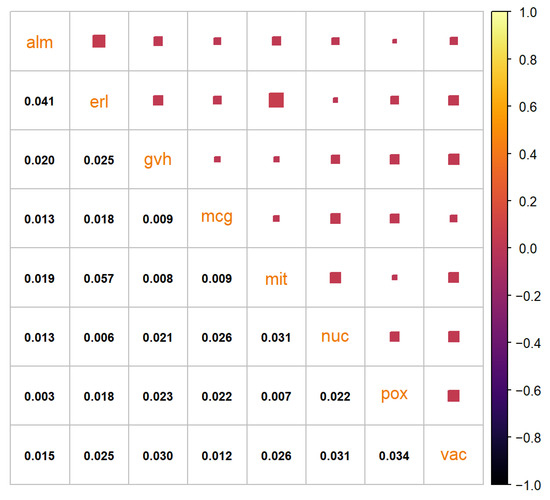
Figure A4.
Residual correlation matrix of the synthetic “yeast” data set generated by the benchmark method.
Table A2.
Table of p-values calculated by the Anderson–Darling and DTS statistical tests comparing the distributions of the attributes of the real-life “yeast” data set and the attributes of the synthetic data set generated by the benchmark method.
Table A2.
Table of p-values calculated by the Anderson–Darling and DTS statistical tests comparing the distributions of the attributes of the real-life “yeast” data set and the attributes of the synthetic data set generated by the benchmark method.
| Attribute | Anderson–Darling | DTS |
|---|---|---|
| mcg | 0.7715 | 0.7390 |
| gvh | 0.8530 | 0.5705 |
| alm | 0.9485 | 0.8020 |
| mit | 0.6165 | 0.7790 |
| erl | 0.0025 | 0.0615 |
| pox | 0.0020 | 0.0530 |
| vac | 0.6205 | 0.2050 |
| nuc | 0.2915 | 0.8525 |
The synthetic data set generated by the cluster preserving method can be seen in Figure A5. Even though it is not immediately evident, the spatial distribution of the synthetic data is closer to that of the real-life data. The synthetic data set has 1483 data points. The quantiles of the synthetic data set correspond to the quantiles of the real-life data set, as can be seen in Figure A6. As with the “texture” data set, using the cluster preserving method to generate the synthetic “yeast” data set results in smaller correlation residuals, as evidenced by Figure A7. The sum of residuals above the main diagonal is and the average residual value is —both a significant reduction from the residual values of the synthetic data set generated by the benchmark method. However, the apparent improvement in correlation matrix residuals is absent from the p-values in Table A3.
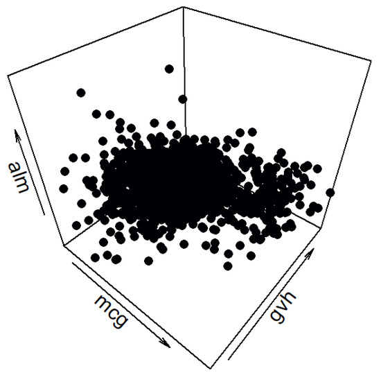
Figure A5.
Three-dimensional view of the synthetic “yeast” data set generated by the cluster preserving method.
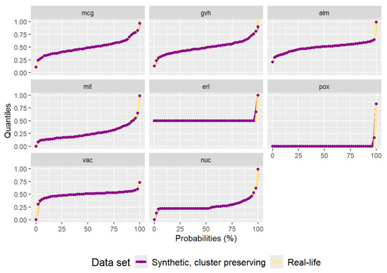
Figure A6.
Plot of quantiles calculated for the real-life “yeast” data set and the synthetic data set generated by the cluster preserving method.

Figure A7.
Residual correlation matrix of the synthetic “yeast” data set generated by the cluster preserving method.
Table A3.
Table of p-values calculated by the Anderson–Darling and DTS statistical tests comparing the distributions of the attributes of the real-life “yeast” data set and the attributes of the synthetic data set generated by the cluster preserving method.
Table A3.
Table of p-values calculated by the Anderson–Darling and DTS statistical tests comparing the distributions of the attributes of the real-life “yeast” data set and the attributes of the synthetic data set generated by the cluster preserving method.
| Attribute | Anderson–Darling | DTS |
|---|---|---|
| mcg | 0.7805 | 0.7450 |
| gvh | 0.8515 | 0.5760 |
| alm | 0.9555 | 0.7910 |
| mit | 0.6370 | 0.7785 |
| erl | 0.0005 | 0.0620 |
| pox | 0.0045 | 0.0465 |
| vac | 0.6410 | 0.1965 |
| nuc | 0.3130 | 0.8315 |
The densities of each attribute in the three data sets can be seen in Figure A8. There are clear similarities between the “yeast” data set and the “texture” data set when comparing the effects of data generation. All the densities of the three data sets are nearly impossible to separate from one another. Furthermore, the results of the statistical tests in Table A4 and Table A5 show the heterogeneous nature of the data set.
Table A4.
Table of p-values calculated by the Anderson–Darling statistical test comparing the distributions of each of the attributes (“Attr.” in table) of the real-life data set and the synthetic data set (cluster preserving method) depending on the class (“Cls.” in table).
Table A4.
Table of p-values calculated by the Anderson–Darling statistical test comparing the distributions of each of the attributes (“Attr.” in table) of the real-life data set and the synthetic data set (cluster preserving method) depending on the class (“Cls.” in table).
| Anderson–Darling | |||||||||||
|---|---|---|---|---|---|---|---|---|---|---|---|
| Cls. | CYT | ERL | EXC | ME1 | ME2 | ME3 | MIT | NUC | POX | VAC | |
| Attr. | |||||||||||
| mcg | 0.972 | 0.424 | 0.622 | 0.975 | 0.764 | 0.538 | 0.707 | 0.922 | 0.769 | 0.316 | |
| gvh | 0.958 | 0.318 | 0.886 | 0.626 | 0.500 | 0.517 | 0.743 | 0.986 | 0.692 | 0.364 | |
| alm | 0.947 | 0.311 | 0.990 | 0.747 | 0.560 | 0.497 | 0.846 | 0.942 | 0.897 | 0.541 | |
| mit | 0.987 | 0.290 | 0.844 | 0.845 | 0.521 | 0.562 | 0.828 | 0.970 | 0.827 | 0.146 | |
| erl | 0.264 | 1.000 | 1.000 | 1.000 | 0.020 | 0.067 | 1.000 | 0.240 | 1.000 | 1.000 | |
| pox | 0.039 | 1.000 | 1.000 | 1.000 | 1.000 | 1.000 | 0.304 | 1.000 | 0.006 | 1.000 | |
| vac | 0.936 | 1.000 | 0.838 | 0.464 | 0.810 | 0.316 | 0.714 | 0.928 | 0.350 | 0.122 | |
| nuc | 0.658 | 0.408 | 0.330 | 0.806 | 0.238 | 0.616 | 0.807 | 0.983 | 0.006 | 0.010 | |
Table A5.
Table of p-values calculated by the DTS statistical test comparing the distributions of each of the attributes (“Attr.” in table) of the real-life data set and the synthetic data set (cluster preserving method) depending on the class (“Cls.” in table).
Table A5.
Table of p-values calculated by the DTS statistical test comparing the distributions of each of the attributes (“Attr.” in table) of the real-life data set and the synthetic data set (cluster preserving method) depending on the class (“Cls.” in table).
| DTS | |||||||||||
|---|---|---|---|---|---|---|---|---|---|---|---|
| Cls. | CYT | ERL | EXC | ME1 | ME2 | ME3 | MIT | NUC | POX | VAC | |
| Attr. | |||||||||||
| mcg | 0.970 | 0.386 | 0.929 | 0.909 | 0.903 | 0.576 | 0.848 | 0.760 | 0.706 | 0.383 | |
| gvh | 0.885 | 0.278 | 0.954 | 0.651 | 0.493 | 0.427 | 0.428 | 0.983 | 0.912 | 0.337 | |
| alm | 0.722 | 0.277 | 0.989 | 0.579 | 0.768 | 0.785 | 0.800 | 0.901 | 0.853 | 0.299 | |
| mit | 0.914 | 0.388 | 0.961 | 0.426 | 0.606 | 0.786 | 0.836 | 0.773 | 0.705 | 0.178 | |
| erl | 0.355 | 1.000 | 1.000 | 1.000 | 0.083 | 0.141 | 1.000 | 0.337 | 1.000 | 1.000 | |
| pox | 0.136 | 1.000 | 1.000 | 1.000 | 1.000 | 1.000 | 0.336 | 1.000 | 0.034 | 1.000 | |
| vac | 0.728 | 1.000 | 0.888 | 0.418 | 0.728 | 0.566 | 0.262 | 0.528 | 0.402 | 0.272 | |
| nuc | 0.938 | 0.600 | 0.749 | 0.419 | 0.364 | 0.587 | 0.513 | 0.875 | 0.267 | 0.187 | |
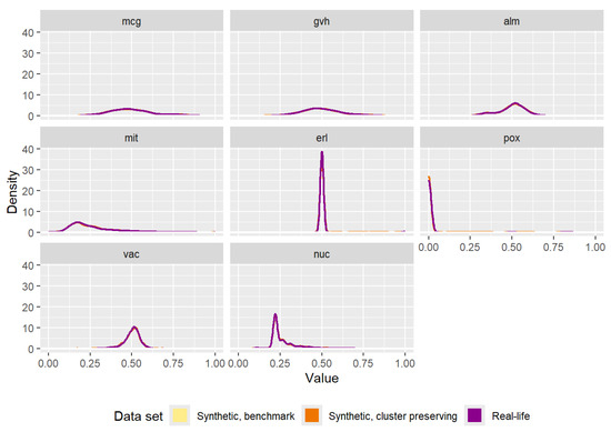
Figure A8.
Comparison of the densities of the attributes of the real-life data set and the attributes of the synthetic data sets (one generated by the benchmark method, the other generated by the cluster preserving method).
Appendix A.1. Downstream Task—Classification
To test the hypothesis a model could be trained on the synthetic data generated by the cluster preserving method and then evaluated on the real-life data set, a simple classification was performed using Support Vector Machines (SVM) from the R package “e1071” (“Misc Functions of the Department of Statistics, Probability Theory Group (Formerly: E1071), TU Wien.”, https://cran.r-project.org/web/packages/e1071/e1071.pdf, accessed on 25 April 2025). Both the real-life data set and the synthetic data set generated by the cluster preserving method were split into training and testing subsets, with of the data set being used for training and the remainder for testing. All the attributes were used to predict the class and no further optimizations were implemented.
Evaluating the model trained on the real-life training set on the real-life test set yielded an accuracy of . Evaluating the model trained on the synthetic training set on the synthetic test set yielded an accuracy of . Finally, evaluating the model trained on the synthetic training set on the real-life test set yielded an accuracy of . These results indicate the hypothesis that the synthetic data generated by the cluster preserving method can be used to train a model that can then function well with real-life data holds.
Appendix B. Additional Graphs for the “Texture” Data Set
As was stated in Section 4, only a selection of variables and classes of the full real-life data set was used to make the results visually interpretable. This section provides more detailed three-dimensional graphs to further illustrate the differences between the benchmark method (Section 2.2.2) and the cluster preserving method (Section 3).
Figure A9 shows four different views of the filtered real-life data set. Each of the four different classes is presented in a different color to make it more easily distinguishable from the others. Variables ‘V10’ and ‘V23’ were chosen as the x- and y-axis because they provide the most open and easily interpretable plane. The additional four variables are used as the z-axis to provide more comprehensive views. Graphs (a,b) show that even the filtered classes have a certain amount of overlap, depending on how the data points are plotted.
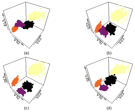
Figure A9.
Three-dimensional view of classes selected from “texture” data set. Plotted with different z-axes.
Figure A10 shows four different views of the synthetic data set generated by the benchmark method. As can be seen, the synthetic data roughly follow the orientation of the real-life data, and, in some cases (graph (c)), even mostly replicate the layout of the real-life data set. However, this method produces multiple artifacts as well, which result in data points being present in places the filtered real-life data set does not have any.
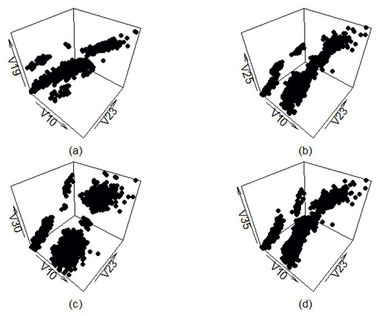
Figure A10.
Three-dimensional view of classes generated by the benchmark method. Plotted with different z-axes.
Figure A11 shows four different views of the synthetic data set generated by the cluster preserving method. There is very little visual difference between this data set and the filtered real-life data set (apart from the classes being of different color in Figure A9). The cluster shapes do not correspond to the cluster shapes of the real-life data set completely, but that is expected and even desired. It is likely the generated data points are not present in the real-life data set, indicating that using data generated by the cluster preserving method to test the abilities of machine learning or clustering methods could be worthwhile.
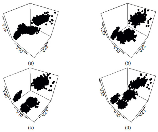
Figure A11.
Three-dimensional view of classes generated by the cluster preserving method. Plotted with different z-axes.
References
- Chen, R.J.; Lu, M.Y.; Chen, T.Y.; Williamson, D.F.K.; Mahmood, F. Synthetic data in machine learning for medicine and healthcare. Nat. Biomed. Eng. 2021, 5, 493–497. [Google Scholar] [CrossRef] [PubMed]
- Liu, Q.; Khalil, M.; Jovanovic, J.; Shakya, R. Scaling While Privacy Preserving: A Comprehensive Synthetic Tabular Data Generation and Evaluation in Learning Analytics. In Proceedings of the 14th Learning Analytics and Knowledge Conference, Kyoto, Japan, 18–24 March 2024; LAK ’24. pp. 620–631. [Google Scholar] [CrossRef]
- Morley-Fletcher, E. New Solutions to Biomedical Data Sharing: Secure Computation and Synthetic Data. In Personalized Medicine in the Making: Philosophical Perspectives from Biology to Healthcare; Beneduce, C., Bertolaso, M., Eds.; Springer International Publishing: Cham, Switzerland, 2022; pp. 173–189. [Google Scholar] [CrossRef]
- Giuffrè, M.; Shung, D.L. Harnessing the power of synthetic data in healthcare: Innovation, application, and privacy. NPJ Digit. Med. 2023, 6, 186. [Google Scholar] [CrossRef] [PubMed]
- Potluru, V.K.; Borrajo, D.; Coletta, A.; Dalmasso, N.; El-Laham, Y.; Fons, E.; Ghassemi, M.; Gopalakrishnan, S.; Gosai, V.; Kreačić, E.; et al. Synthetic Data Applications in Finance. arXiv 2024, arXiv:2401.00081. [Google Scholar] [CrossRef]
- Ruscio, J.; Kaczetow, W. Simulating multivariate nonnormal data using an iterative algorithm. Multivar. Behav. Res. 2008, 43, 355–381. [Google Scholar] [CrossRef]
- Petricioli, L.; Humski, L.; Vranić, M.; Pintar, D. Data Set Synthesis Based on Known Correlations and Distributions for Expanded Social Graph Generation. IEEE Access 2020, 8, 33013–33022. [Google Scholar] [CrossRef]
- Iftikhar, N.; Liu, X.; Nordbjerg, F.E.; Danalachi, S. A Prediction-Based Smart Meter Data Generator. In Proceedings of the 19th International Conference on Network-Based Information Systems, NBiS 2016, Ostrava, Czech Republic, 7–9 September 2016; pp. 173–180. [Google Scholar] [CrossRef]
- Syahaneim; Hazwani, R.A.; Wahida, N.; Shafikah, S.I.; Zuraini; Ellyza, P.N. Automatic Artificial Data Generator: Framework and implementation. In Proceedings of the 1st International Conference on Information and Communication Technology, ICICTM 2016, Kuala Lumpur, Malaysia, 16–17 May 2016; IEEE: Piscataway, NJ, USA, 2017; pp. 56–60. [Google Scholar] [CrossRef]
- Liu, R.; Fang, B.; Tang, Y.Y.; Chan, P.P. Synthetic data generator for classification rules learning. In Proceedings of the 7th International Conference on Cloud Computing and Big Data, CCBD 2016, Macau, China, 16–18 November 2016; IEEE: Piscataway, NJ, USA, 2017; pp. 357–361. [Google Scholar] [CrossRef]
- Nowok, B.; Raab, G.M.; Dibben, C. Synthpop: Bespoke creation of synthetic data in R. J. Stat. Softw. 2016, 74, 1–26. [Google Scholar] [CrossRef]
- Robnik-Sikonja, M. Data Generators for Learning Systems Based on RBF Networks. IEEE Trans. Neural Netw. Learn. Syst. 2016, 27, 926–938. [Google Scholar] [CrossRef]
- Sagduyu, Y.E.; Grushin, A.; Shi, Y. Synthetic social media data generation. IEEE Trans. Comput. Soc. Syst. 2018, 5, 605–620. [Google Scholar] [CrossRef]
- Yang, S.; Zhou, Y.; Guo, Y.; Farneth, R.A.; Marsic, I.; Randall, B.S. Semi-Synthetic Trauma Resuscitation Process Data Generator. In Proceedings of the IEEE International Conference on Healthcare Informatics, ICHI 2017, Park City, UT, USA, 23–26 August 2017; IEEE: Piscataway, NJ, USA, 2017; p. 573. [Google Scholar] [CrossRef]
- Xu, L.; Veeramachaneni, K. Synthesizing Tabular Data using Generative Adversarial Networks. arXiv 2018, arXiv:1811.11264. [Google Scholar]
- Xu, L.; Skoularidou, M.; Cuesta-Infante, A.; Veeramachaneni, K. Modeling tabular data using conditional GAN. In Proceedings of the 33rd International Conference on Neural Information Processing Systems, Vancouver, BC, Canada, 8–14 December 2019; Curran Associates Inc.: Red Hook, NY, USA, 2019. Number 659. pp. 7335–7345. [Google Scholar]
- Zhao, Z.; Kunar, A.; Birke, R.; Chen, L.Y. CTAB-GAN: Effective Table Data Synthesizing. In Proceedings of the 13th Asian Conference on Machine Learning, Virtual, 17–19 November 2021; PMLR: New York, NY, USA, 2021; pp. 97–112. [Google Scholar]
- Rajabi, A.; Garibay, O.O. TabFairGAN: Fair Tabular Data Generation with Generative Adversarial Networks. Mach. Learn. Knowl. Extr. 2022, 4, 22. [Google Scholar] [CrossRef]
- Rai, R.; Sural, S. Tool/Dataset Paper: Realistic ABAC Data Generation using Conditional Tabular GAN. In Proceedings of the 13th ACM Conference on Data and Application Security and Privacy, Charlotte, NC, USA, 24–26 April 2023; pp. 273–278. [Google Scholar] [CrossRef]
- He, G.; Zhao, Y.; Yan, C. Application of tabular data synthesis using generative adversarial networks on machine learning-based multiaxial fatigue life prediction. Int. J. Press. Vessel. Pip. 2022, 199, 104779. [Google Scholar] [CrossRef]
- Gao, N.; Xue, H.; Shao, W.; Zhao, S.; Qin, K.K.; Prabowo, A.; Rahaman, M.S.; Salim, F.D. Generative Adversarial Networks for Spatio-temporal Data: A Survey. ACM Trans. Intell. Syst. Technol. 2022, 13, 22:1–22:25. [Google Scholar] [CrossRef]
- Liu, T.; Fan, J.; Li, G.; Tang, N.; Du, X. Tabular data synthesis with generative adversarial networks: Design space and optimizations. VLDB J. 2023, 33, 255–280. [Google Scholar] [CrossRef]
- Zhou, Y.; Qi, J. Synthesizing Tabular Data Using Selectivity Enhanced Generative Adversarial Networks. arXiv 2025, arXiv:2502.21034. [Google Scholar] [CrossRef]
- Suh, N.; Lin, X.; Hsieh, D.Y.; Honarkhah, M.; Cheng, G. AutoDiff: Combining Auto-encoder and Diffusion model for tabular data synthesizing. arXiv 2023, arXiv:2310.15479. [Google Scholar] [CrossRef]
- Anshelevich, D.; Katz, G. Synthetic Tabular Data Generation Using a Vae-Gan Architecture. 2024. Available online: https://papers.ssrn.com/sol3/papers.cfm?abstract_id=4902016 (accessed on 13 March 2025).
- Tazwar, S.; Knobbout, M.; Quesada, E.; Popa, M. Tab-VAE: A Novel VAE for Generating Synthetic Tabular Data. In Proceedings of the 13th International Conference on Pattern Recognition Applications and Methods, Rome, Italy, 24–26 February 2024; pp. 17–26. [Google Scholar] [CrossRef]
- Wang, A.X.; Nguyen, B.P. Deterministic Autoencoder using Wasserstein loss for tabular data generation. Neural Netw. 2025, 185, 107208. [Google Scholar] [CrossRef] [PubMed]
- Borisov, V.; Sessler, K.; Leemann, T.; Pawelczyk, M.; Kasneci, G. Language Models are Realistic Tabular Data Generators. In Proceedings of the 11th International Conference on Learning Representations, Kigali, Rwanda, 1–5 May 2023. [Google Scholar]
- Wang, Y.; Feng, D.; Dai, Y.; Chen, Z.; Huang, J.; Ananiadou, S.; Xie, Q.; Wang, H. HARMONIC: Harnessing LLMs for Tabular Data Synthesis and Privacy Protection. In Proceedings of the 38th Conference on Neural Information Processing Systems, Datasets and Benchmarks Track, Vancouver, BC, Canada, 10–15 December 2024. [Google Scholar]
- Cromp, S.; GNVV, S.S.S.N.; Alkhudhayri, M.; Cao, C.; Guo, S.; Roberts, N.; Sala, F. Tabby: Tabular Data Synthesis with Language Models. arXiv 2025, arXiv:2503.02152. [Google Scholar] [CrossRef]
- Zhao, Z.; Birke, R.; Chen, L. TabuLa: Harnessing Language Models for Tabular Data Synthesis. arXiv 2025, arXiv:2310.12746. [Google Scholar] [CrossRef]
- Ayala-Rivera, V.; McDonagh, P.; Cerqueus, T.; Murphy, L. Synthetic Data Generation using Benerator Tool. arXiv 2013. [Google Scholar] [CrossRef]
- Eno, J.; Thompson, C.W. Generating synthetic data to match data mining patterns. IEEE Internet Comput. 2008, 12, 78–82. [Google Scholar] [CrossRef]
- Erling, O.; Averbuch, A.; Larriba-Pey, J.; Chafi, H.; Gubichev, A.; Prat, A.; Pham, M.D.; Boncz, P. The LDBC social network benchmark: Interactive workload. In Proceedings of the ACM SIGMOD International Conference on Management of Data, Melbourne, VIC, Australia, 31 May–4 June 2015; pp. 619–630. [Google Scholar] [CrossRef]
- Hoag, J.E.; Thompson, C.W. A Parallel General-Purpose Synthetic Data Generator. SIGMOD Rec. 2007, 36, 19–24. [Google Scholar] [CrossRef]
- Jeske, D.R.; Lin, P.J.; Rendón, C.; Xiao, R.; Samadi, B. Synthetic data generation capabilities for testing data mining tools. In Proceedings of the IEEE Military Communications Conference MILCOM, Washington, DC, USA, 23–25 October 2006; IEEE: Piscataway, NJ, USA, 2007; pp. 1–6. [Google Scholar] [CrossRef]
- Khan, J.; Lee, S. Online Social Networks (OSN) evolution model based on homophily and preferential attachment. Symmetry 2018, 10, 654. [Google Scholar] [CrossRef]
- Maciejewski, R.; Hafen, R.; Rudolph, S.; Tebbetts, G.; Cleveland, W.S.; Grannis, S.J.; Ebert, D.S. Generating synthetic syndromic-surveillance data for evaluating visual-analytics techniques. IEEE Comput. Graph. Appl. 2009, 29, 18–28. [Google Scholar] [CrossRef] [PubMed]
- Nettleton, D.F. A synthetic data generator for online social network graphs. Soc. Netw. Anal. Min. 2016, 6, 44. [Google Scholar] [CrossRef]
- Petermann, A.; Junghanns, M.; Müller, R.; Rahm, E. FoodBroker-Generating synthetic datasets for Graph-Based business analytics. In Big Data Benchmarking; Lecture Notes in Computer Science (Including Subseries Lecture Notes in Artificial Intelligence and Lecture Notes in Bioinformatics); Springer: Cham, Switzerland, 2015; Volume 8991, pp. 145–155. [Google Scholar] [CrossRef]
- Pham, M.D.; Boncz, P.; Erling, O. S3G2: A scalable structure-correlated social graph generator. In Selected Topics in Performance Evaluation and Benchmarking; Lecture Notes in Computer Science (Including Subseries Lecture Notes in Artificial Intelligence and Lecture Notes in Bioinformatics); Springer: Berlin/Heidelberg, Germany, 2013; Volume 7755, pp. 156–172. [Google Scholar] [CrossRef]
- Spasić, M.; Jovanovik, M.; Prat-Pérez, A. An RDF dataset generator for the social network benchmark with real-world coherence. CEUR Workshop Proc. 2016, 1700, 1–8. [Google Scholar]
- Lee, J.; Hong, J.; Hong, B.; Ahn, J. A generator of test data set for tactical moving objects based on velocity. In Proceedings of the IEEE International Conference on Big Data, Big Data 2016, Washington, DC, USA, 5–8 December 2016; pp. 4011–4013. [Google Scholar] [CrossRef]
- Pérez-Rosés, H.; Sebé, F. Synthetic generation of social network data with endorsements. J. Simul. 2015, 9, 279–286. [Google Scholar] [CrossRef]
- Vale, C.D.; Maurelli, V.A. Simulating multivariate nonnormal distributions. Psychometrika 1983, 48, 465–471. [Google Scholar] [CrossRef]
- Eigenschink, P.; Reutterer, T.; Vamosi, S.; Vamosi, R.; Sun, C.; Kalcher, K. Deep Generative Models for Synthetic Data: A Survey. IEEE Access 2023, 11, 47304–47320. [Google Scholar] [CrossRef]
- Rohlfs, C. Generalization in neural networks: A broad survey. Neurocomputing 2025, 611, 128701. [Google Scholar] [CrossRef]
- Wang, A.X.; Chukova, S.S.; Simpson, C.R.; Nguyen, B.P. Challenges and opportunities of generative models on tabular data. Appl. Soft Comput. 2024, 166, 112223. [Google Scholar] [CrossRef]
- Goyal, M.; Mahmoud, Q.H. A Systematic Review of Synthetic Data Generation Techniques Using Generative AI. Electronics 2024, 13, 3509. [Google Scholar] [CrossRef]
- Perković, G.; Drobnjak, A.; Botički, I. Hallucinations in LLMs: Understanding and Addressing Challenges. In Proceedings of the 47th MIPRO ICT and Electronics Convention (MIPRO), Opatija, Croatia, 20–24 May 2024; pp. 2084–2088. [Google Scholar] [CrossRef]
- Xu, Z.; Jain, S.; Kankanhalli, M. Hallucination is Inevitable: An Innate Limitation of Large Language Models. arXiv 2025, arXiv:2401.11817. [Google Scholar] [CrossRef]
- Miyato, T.; Koyama, M. cGANs with Projection Discriminator. arXiv 2018, arXiv:1802.05637. [Google Scholar] [CrossRef]
- Raghunathan, T.E. Synthetic Data. Annu. Rev. Stat. Its Appl. 2021, 8, 129–140. [Google Scholar] [CrossRef]
- Wang, Z.; Myles, P.; Tucker, A. Generating and evaluating cross-sectional synthetic electronic healthcare data: Preserving data utility and patient privacy. Comput. Intell. 2021, 37, 819–851. [Google Scholar] [CrossRef]
- Hosain, M.T.; Jim, J.R.; Mridha, M.F.; Kabir, M.M. Explainable AI approaches in deep learning: Advancements, applications and challenges. Comput. Electr. Eng. 2024, 117, 109246. [Google Scholar] [CrossRef]
- Zhao, H.; Chen, H.; Yang, F.; Liu, N.; Deng, H.; Cai, H.; Wang, S.; Yin, D.; Du, M. Explainability for Large Language Models: A Survey. ACM Trans. Intell. Syst. Technol. 2024, 15, 20:1–20:38. [Google Scholar] [CrossRef]
- Ruscio, J.; Ruscio, A.M.; Meron, M. Applying the bootstrap to taxometric analysis: Generating empirical sampling distributions to help interpret results. Multivar. Behav. Res. 2007, 42, 349–386. [Google Scholar] [CrossRef] [PubMed]
- Humski, L.; Pintar, D.; Vranić, M. Analysis of Facebook Interaction as Basis for Synthetic Expanded Social Graph Generation. IEEE Access 2019, 7, 6622–6636. [Google Scholar] [CrossRef]
- Dowd, C. A new ECDF Two-Sample test statistic. arXiv 2020, arXiv:2007.01360. [Google Scholar] [CrossRef]
- Anderson, T.W.; Darling, D.A. Asymptotic Theory of Certain “Goodness of Fit” Criteria Based on Stochastic Processes. Ann. Math. Stat. 1952, 23, 193–212. [Google Scholar] [CrossRef]
Disclaimer/Publisher’s Note: The statements, opinions and data contained in all publications are solely those of the individual author(s) and contributor(s) and not of MDPI and/or the editor(s). MDPI and/or the editor(s) disclaim responsibility for any injury to people or property resulting from any ideas, methods, instructions or products referred to in the content. |
© 2025 by the authors. Licensee MDPI, Basel, Switzerland. This article is an open access article distributed under the terms and conditions of the Creative Commons Attribution (CC BY) license (https://creativecommons.org/licenses/by/4.0/).