MESC-DETR: An Improved RT-DETR Algorithm for Steel Surface Defect Detection

Abstract

Accurate detection of steel surface defects is crucial for ensuring safety and efficiency in steel production. In this study, we propose a multi-scale edge-enhanced structured composite detection Transformer (MESC-DETR) based on the RT-DETR framework for steel surface defect detection. Three primary improvements are introduced, as follows: (1) a Composite-ConvNeXtV2 backbone network architecture is developed, which integrates ConvNeXtV2 networks through a dense higher-level composition (DHLC) method to enhance multi-scale feature extraction capabilities; (2) an edge enhancement module (EEM) is proposed, incorporating a scale sequence feature fusion (SSFF) structure to design an edge-enhanced feature fusion (EEFF) architecture, thereby improving multi-scale defect detection and edge information perception; (3) a novel Focal-MPDIoU loss function is formulated by optimizing focal loss and MPDIoU, which further enhances model convergence speed and localization accuracy. Experimental results demonstrate that on GC10-DET and NEU-DET datasets, the proposed algorithm achieves 7.2% and 3.7% improvements in mean average precision (mAP) at IoU = 0.50, along with 2.9% and 1.5% mAP enhancements under IoU = 0.50:0.95. These findings indicate that MESC-DETR exhibits superior performance in steel surface defect detection, holding significant implications for steel manufacturing processes.

1. Introduction

The issue of overcapacity in the global steel industry is becoming increasingly prominent, primarily due to the slowdown in global economic growth, which results in lackluster demand growth, making capacity difficult to absorb in the short term. Steel companies face intense competition and operational pressure, necessitating measures such as reducing production costs, improving product quality, and achieving intelligent and standardized production to address these challenges. Moreover, steel production often encounters issues related to continuity, smoothness, and uniformity, such as rolling scale, blotches, inclusions, cracking, dents, and scratches [1], which are surface defects affecting not only the appearance quality of steel but also its mechanical and corrosion resistance properties, thereby reducing the lifespan and safety of related industrial products. The causes of these defects include improper control of smelting temperature, raw material quality issues, operational errors, and process defects. Therefore, efficiently and intelligently detecting defects during steel production is critical for enhancing production efficiency and quality.

With the continuous advancement of computer vision technologies and hardware devices, increasing scholarly attention has been directed toward deep learning-based steel surface defect detection methodologies. Existing research predominantly focuses on object detection frameworks that simultaneously achieve defect localization and classification while meeting real-time operational requirements in production environments. However, significant limitations persist in current approaches. Primarily, mainstream deep learning-based detection models, originally developed for natural scene objects (e.g., household items, vehicles, and humans), face substantial challenges when applied to steel surface defects characterized by intricate morphological contours and complex textural patterns. Current technical implementations in this specialized domain remain underexplored, particularly in comprehensive feature extraction from industrial datasets. To address this critical gap, this study proposes an optimized backbone network architecture specifically designed to enhance defect feature representation capabilities. Furthermore, prior investigations have inadequately addressed the unique characteristics of steel defects, including edge ambiguity and extreme scale variations within individual specimens. In response, we developed an edge-enhanced feature fusion (EEFF) module to improve multi-scale defect detection and edge perception, complemented by a novel loss function, Focal-MPDIoU, to refine detection accuracy. By strategically modifying the real-time RT-DETR detection framework, our methodology achieves an optimal balance between detection precision and computational efficiency, demonstrating superior performance in practical industrial applications. In conclusion, this study’s main contributions are summarized as follows:

• We employ ConvNeXtV2 as the backbone network of MESC-DETR and incorporate a DHLC structure, thereby proposing a novel composite backbone network termed Composite-ConvNeXtV2 (C-ConvNeXt). The proposed architecture significantly enhances the feature extraction capability of the model and improves detection performance for small-scale defects. Experimental validation on the GC10-DET benchmark demonstrates that these improvements yield a 3.4% increase in mAP50 compared to baseline configurations.
• We introduce a scale sequence feature fusion (SSFF) module to optimize multi-scale feature integration, enabling the detection algorithm to achieve robust performance across defects of varying scales. Furthermore, a bypass edge-enhanced feature fusion architecture is specifically designed within the encoder component of the model to enhance the model’s capability in recognizing defects with ambiguous boundaries. These architectural improvements demonstrate effectiveness through a 1.8% increase in mAP50 on the GC10-DET dataset.
• We optimize the loss function of RT-DETR by integrating focal loss with MPDIoU, proposing a Focal-MPDIoU loss that effectively mitigates the impact of low-quality negative samples while enhancing model convergence rate and object localization accuracy, resulting in a 2.0% improvement in mAP50 on the benchmark.
• We conduct comprehensive evaluations of the MESC-DETR algorithm and its constituent modules on the GC10-DET benchmark, supplemented by generalizability evaluation on the NEU-DET dataset. The proposed method demonstrates mAP50 improvements of 7.2% and 3.7% over RT-DETR on respective datasets, while outperforming state-of-the-art object detection algorithms in model accuracy, validating its superior performance in steel surface defect inspection tasks.

The remainder of this study is organized as follows: Section 2 reviews related studies and discusses their limitations. Section 3 presents the architecture and underlying principles of the proposed MESC-DETR framework. Section 4 presents the experimental validation of the MESC-DETR algorithm, detailing the experimental datasets and evaluation metrics, and providing comparative analyses of the results. Finally, Section 5 concludes this study with key findings and research contributions.

2. Related Works

In order to meet the demands of the steel industry, both domestic and international scholars have conducted extensive research on the detection of surface defects in steel. Currently, most companies use traditional visual inspection methods for steel defect detection. Traditional automated surface inspection systems (ASISs) detect regions of interest (ROI) in images, extract features, and classify defects. These manually designed features include texture features such as the gray level co-occurrence matrix (GLCM) and local binary patterns (LBPs). Typically, multiple features are combined to thoroughly describe defects; however, these methods rely on the expertise of algorithm designers and perform inadequately when faced with complex tasks. Furthermore, as industrial intelligence develops, its detection accuracy no longer meets actual needs. With the development of DL technology, an increasing number of researchers are adopting deep learning algorithms for detecting steel surface defects [2]. Deep learning algorithms boast a broad range of applications and strong scalability, able to adapt to different inspection tasks and scenarios. More importantly, deep neural networks significantly enhance detection accuracy, enabling more precise identification and localization of defects on steel surfaces. Overall, deep learning-based approaches can be divided into two major categories: CNN-based object detection methods and Transformer-based object detection methods. CNN-based methods primarily employ CNN architectures as their backbone, encompassing algorithms that emphasize real-time efficiency, such as YOLOv9 [3] and TTFNet [4], while also including high-precision algorithms exemplified by Cascade R-CNN [5]. Transformer-based methods currently primarily focus on the DETR [6] framework, with notable algorithms including Deformable DETR [7] and DINO [8]. Among existing frameworks, RT-DETR [9] stands out as a promising baseline for industrial defect detection due to its unique design trade-offs. Unlike conventional DETR variants that suffer from high computational complexity, RT-DETR achieves real-time performance through an efficient hybrid encoder–decoder architecture and adaptive feature selection mechanisms. Compared to YOLO series models, RT-DETR eliminates the need for non-maximum suppression (NMS), which is particularly advantageous for detecting densely distributed or overlapping defects—a common challenge in steel surface inspection.

With the advancement of computer vision and artificial intelligence, deep learning-based object detection algorithms have become mainstream, and defect detection has emerged as a critical technology in the field of computer vision, widely utilized in industrial production. Within traditional computer vision approaches, contemporary research efforts are increasingly focused on developing deep neural network architectures tailored for anomaly identification by leveraging domain-specific attributes of inspection datasets. Cao et al. [10] introduced a new method named TAFFNet, which captures multi-scale context through attention convolutional features (ACF), integrates a convolutional block attention module (CBAM) to reduce noise, and incorporates a boundary refinement module to optimize prediction results. This network outperformed 13 advanced methods across three public datasets. Liu et al. [11] proposed a defect detection algorithm for hot-rolled strip steel based on YOLOv5, utilizing deformable convolutional networks (DCNs) and dual attention modules to significantly enhance the detection accuracy for irregular and minute defects, achieving mAP of 0.974 and a speed of 60.51 FPS, outperforming Faster R-CNN, YOLOv3, and other algorithms. Wan et al. [12] introduced the DFINet model, which expands the receptive field through a multi-scale global feature enhancement module (MGFEM) and uses multi-scale features combined with two bidirectional branches and attention modules to filter background information, ultimately generating high-quality defect images. On public datasets, DFINet outperformed 15 advanced methods in effectively detecting strip steel surface defects. Wu et al. [13] proposed a lightweight algorithm combining multi-scale feature fusion attention modules, optimizing the YOLOX architecture to reduce model parameters and computation while improving detection accuracy and speed. On the NEU-DET dataset, the mAP was improved from 76.29% to 81.21%, and the speed from 70.14 FPS to 82.87 FPS. Zhang et al. [14] developed an enhanced YOLOv5s-based detection network, CSWFFN, for hot-rolled steel surface defects. The model utilizes Laplacian sharpening for feature enhancement and introduces an improved BiFPN module, achieving high-precision detection (NEU-DET dataset mAP of 86.8%) and relatively fast speed (51 FPS), with good generalizability on DAGM and MT datasets. Tang et al. [15] presented a method for detecting multi-type, multi-scale surface defects on steel plates based on the Transformer, integrating the Swin Transformer, FPN, RPN, and ROI heads for high precision detection, achieving an mAP of 81.1% on the NEU-DET dataset, outperforming classical methods.

Although these methods have been applied in certain domains, challenges persist due to the diverse types of steel surface defects, significant differences between defect images and traditional object detection images, wide variations in sample scales with both extremely small and large samples, and unclear boundaries. The issues include the following:

• Poor uniformity in defect sample scales, leading to low feature extraction performance and difficulty in precise localization;
• Low contrast between defect edges and background in some samples, resulting in weak edge feature capture in existing technologies and risks of false detection and missed detection;
• Abundance of low-quality negative samples during model training, which can reduce algorithm convergence speed and performance.

To address the aforementioned issues, we proposed an enhanced multi-scale edge-enhanced structured composite DETR (MESC-DETR) algorithm, which is built upon the RT-DETR framework. The proposed method aims to improve the accuracy and robustness of surface defect detection in industrial samples by incorporating a composite backbone network and multi-scale edge enhancement mechanisms.

3. Methods

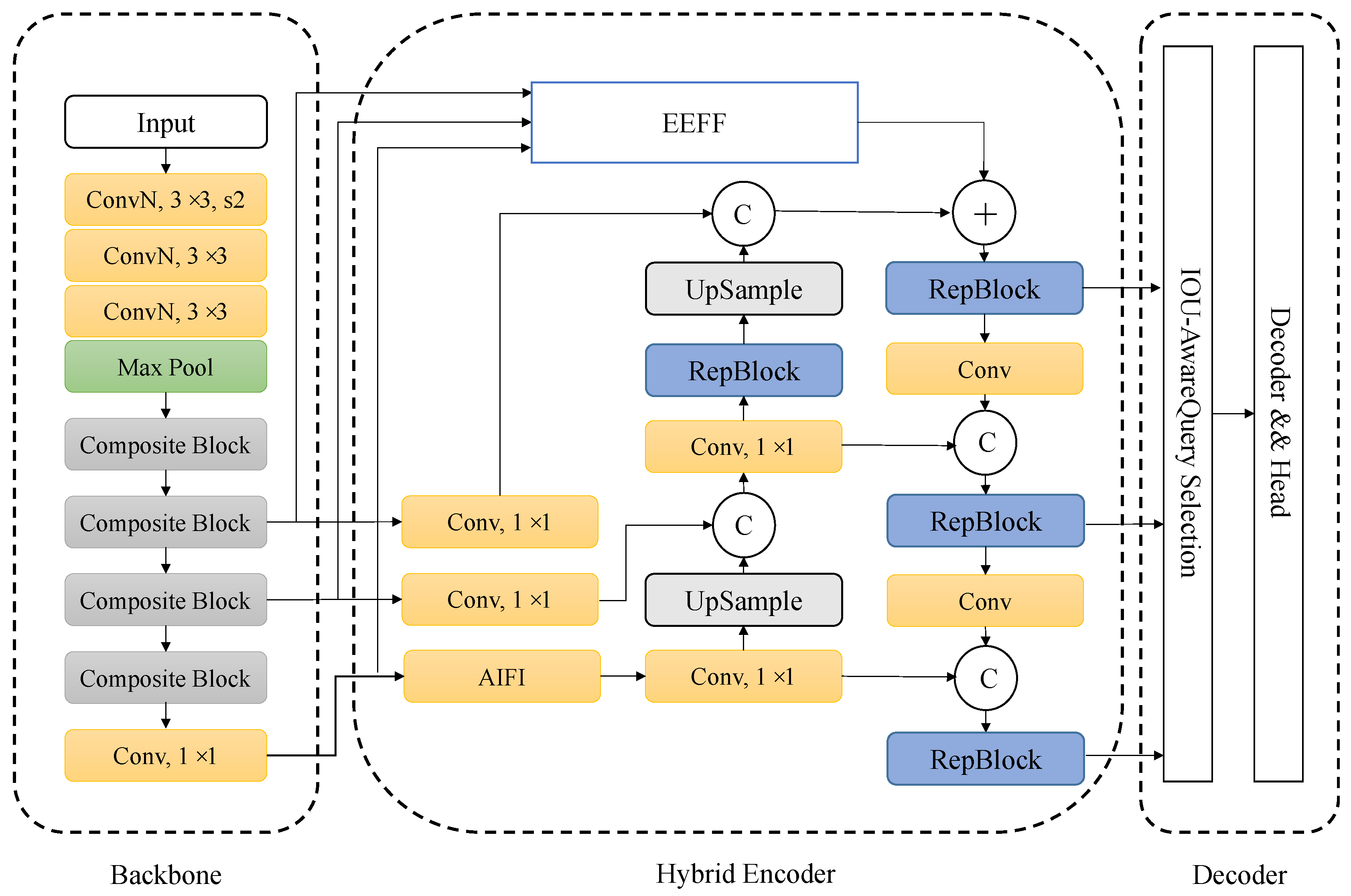
In this section, we provide a detailed introduction to our proposed MESC-DETR model and elaborate on the functional description of each module in the network. First, we present the RT-DETR model, which serves as the foundation of our algorithm. Subsequently, we offer comprehensive descriptions of key enhancements, including the composite backbone structure C-ConvNeXt, the edge-enhanced feature fusion (EEFF) structure, and the improved loss function Focal-MPDIoU loss.

3.1. Overview

The architecture of the improved RT-DETR algorithm (MESC-DETR) proposed in this study is illustrated in Figure 1. The input image is first processed through a series of convolutional layers into the composite block. This block consists of two identical ConvNeXtV2 models connected via the DHLC configuration (detailed architecture can be found in Figure 1. Subsequently, three lower-level feature maps are selected and fed into the edge-enhanced feature fusion (EEFF) structure, which enhances the model’s edge-aware capabilities while improving detection performance for small targets. The EEFF outputs are then combined with the original cross-scale feature fusion (CCFF) structure of RT-DETR to generate fused feature maps. Finally, these fused features, along with the other two outputs from the CCFF structure, are fed into the decoder to produce the final detection results.

3.2. RT-DETR

RT-DETR (real-time detection Transformer) was proposed by Lv et al. [9] in 2023. As a real-time end-to-end object detection model, RT-DETR aims to resolve the speed-accuracy trade-off inherent in conventional detection models (e.g., YOLO series) while simultaneously overcoming the high computational complexity and poor real-time performance limitations of DETR series models. Its core objective is to achieve NMS-free and end-to-end detection through efficient architectural design, fulfilling real-time requirements in industrial applications. The structure of RT-DETR is shown in Figure 2.

3.3. C-ConvNeXt

The original RT-DETR algorithm employs two backbone variants, namely, the classical ResNet network and Baidu’s proprietary HGNetV2, with ResNet being the predominantly adopted version in current implementations. However, through empirical analysis, this study reveals that the baseline RT-DETR configuration demonstrates suboptimal performance in defect image feature learning. This limitation may stem from the significant domain gap between conventional detection datasets (e.g., COCO) and steel defect imagery, coupled with the inadequate transfer learning performance of ResNet-like architectures in industrial defect detection scenarios. Our experimental findings identify that the incorporation of ConvNeXtV2 networks effectively addresses this problem, substantially improving detection performance. Furthermore, by introducing the DHLC structure, we propose the novel Composite-ConvNeXtV2 (C-ConvNeXt) architecture, which significantly increases the backbone’s feature extraction capabilities beyond the baseline ConvNeXtV2.

ConvNeXt (the convolutional network), proposed by Liu et al. [16] in 2020, demonstrated the untapped potential of CNNs by surpassing both Vision Transformers (ViT) and Swin Transformers using a pure CNN architecture. The key modifications include the following: (1) redesigning the block ratio distribution by adjusting the original ResNet-50 configuration from (3,4,6,3) blocks to an optimized (3,3,9,3) arrangement; and (2) revamping the initial convolutional layer with a 4 × 4 kernel and stride 4 to downsample 224 × 224 inputs to 56 × 56 resolution. Furthermore, ConvNeXt enhances network performance through grouped convolution operations and inverted bottleneck structures. ConvNeXtV2 was proposed by Woo et al. [17] in 2023, and serves as the architectural foundation for our redesigned backbone in RT-DETR. The ConvNeXtV2 framework integrates a fully convolutional masked autoencoder (FCMAE) mechanism whose core principle involves randomly masking specific regions of input images and training the model to reconstruct these occluded areas. Compared to conventional masked autoencoder (MAE) architectures, FCMAE replaces fully-connected layers with fully convolutional operations, thereby enhancing feature extraction capabilities without computational overhead inflation. Additionally, FCMAE incorporates multi-scale masking strategies to enable hierarchical feature perception. ConvNeXtV2 further introduces global response normalization (GRN) layers to strengthen inter-channel feature competition through channel-wise excitation mechanisms. Given the specialized training paradigm of FCMAE, our implementation selectively adopts ConvNeXtV2’s backbone architecture while deliberately excluding its self-supervised training methodology. This redesigned backbone demonstrates significantly enhanced defect feature extraction capabilities compared to RT-DETR’s original ResNet and HGNetV2 implementations. The performance advantages of the ConvNeXtV2-based architecture will be empirically validated in subsequent experimental analyses.

In object detection systems, the performance of detection algorithms is predominantly contingent upon the backbone network architecture, where more effective structural designs can yield substantial performance gains. To further enhance the network capabilities beyond ConvNeXtV2, this study introduces the dense higher-level composition (DHLC) methodology for interconnecting dual backbone networks. Originally proposed by Liang et al. [18] in CBNet, the DHLC mechanism enables dense integration of multi-level features from multiple homogeneous backbones. Through progressively expanding receptive fields across cascaded networks, this architectural framework facilitates more effective detection via hierarchical feature integration.

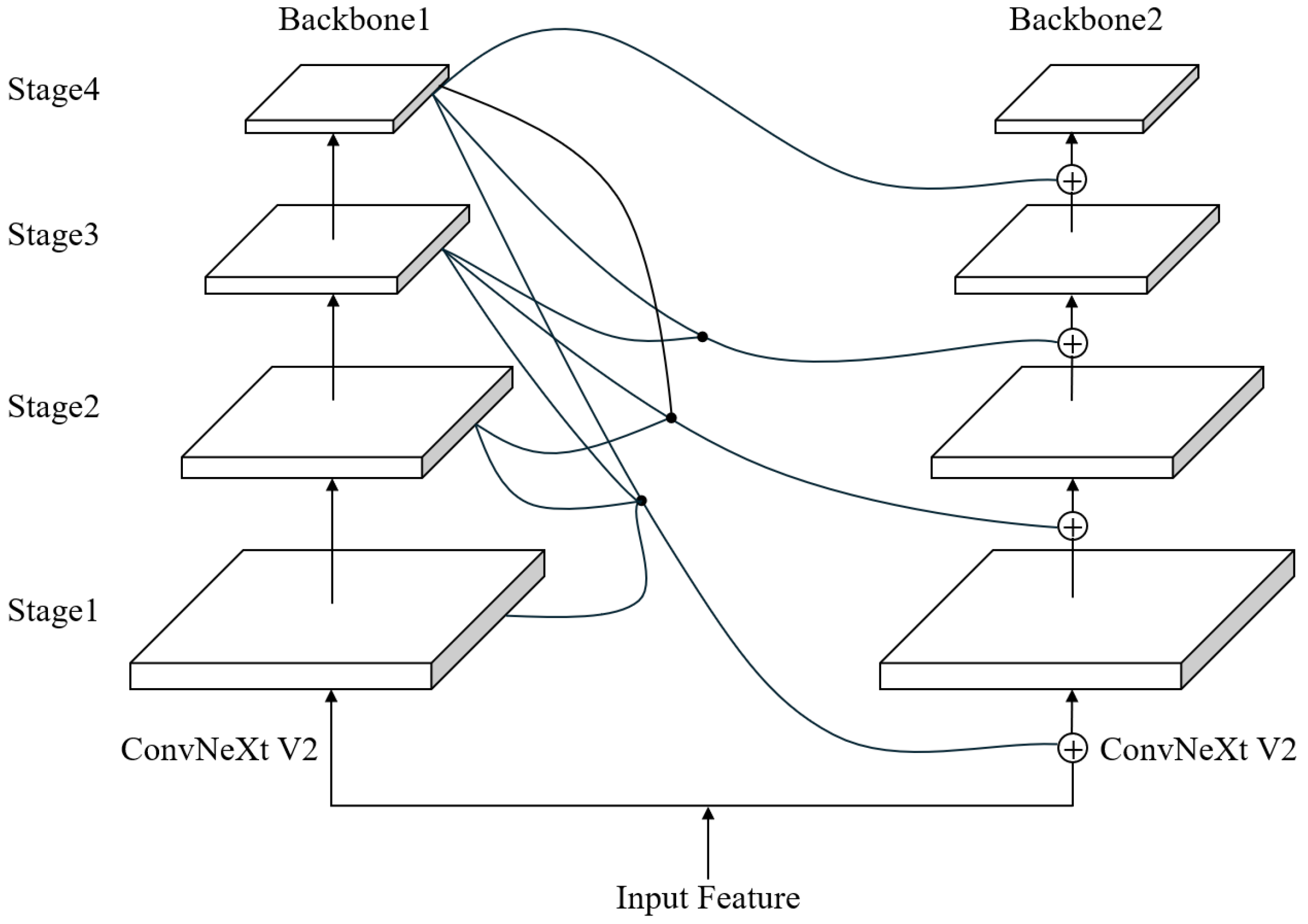
Inspired by this, this study proposes a backbone as Composite-ConvNeXt (C-ConvNeXt), which is formed by combining two ConvNeXtV2 networks through the DHLC connection method, with its architecture illustrated in Figure 3. For the composite connection $g^l(x)$, it takes $x=\{x^i\mid i=1,2,\dots ,L\}$ from the previous auxiliary backbone as input and outputs a feature of the same size as $x^l$. The specific operations of DHLC are detailed in (1). Here, each backbone model consists of L stages, where $Conv$ denotes a $1\times 1$ convolutional layer, and $GN$ represents a group normalization layer. For example, in the left backbone network, each layer is upsampled to the same resolution and summed with the input feature maps. These combined results then undergo convolution and group normalization ($GN$) to form the first-layer output of the right backbone network. Finally, this processed output is fed into the subsequent EEFF architecture as part of its input features.

$$g^l(x)=\sum _{i=l+1}^{L}upsample(GN\left(Con{v}_i\left(x^i\right)\right)),l\ge 1$$

(1)

Composite-ConvNeXt combines higher-level features from the previous backbone network and incorporates them into lower-level layers of the subsequent backbone. this study employs Composite-ConvNeXt to replace the original feature extraction backbone in RT-DETR, thereby enhancing the global defect feature acquisition capability. In the experimental section that follows, we will analyze the rationality of backbone replacement and investigate the performance and speed characteristics of composite structures with varying numbers of backbone components.

3.4. EEFF Module

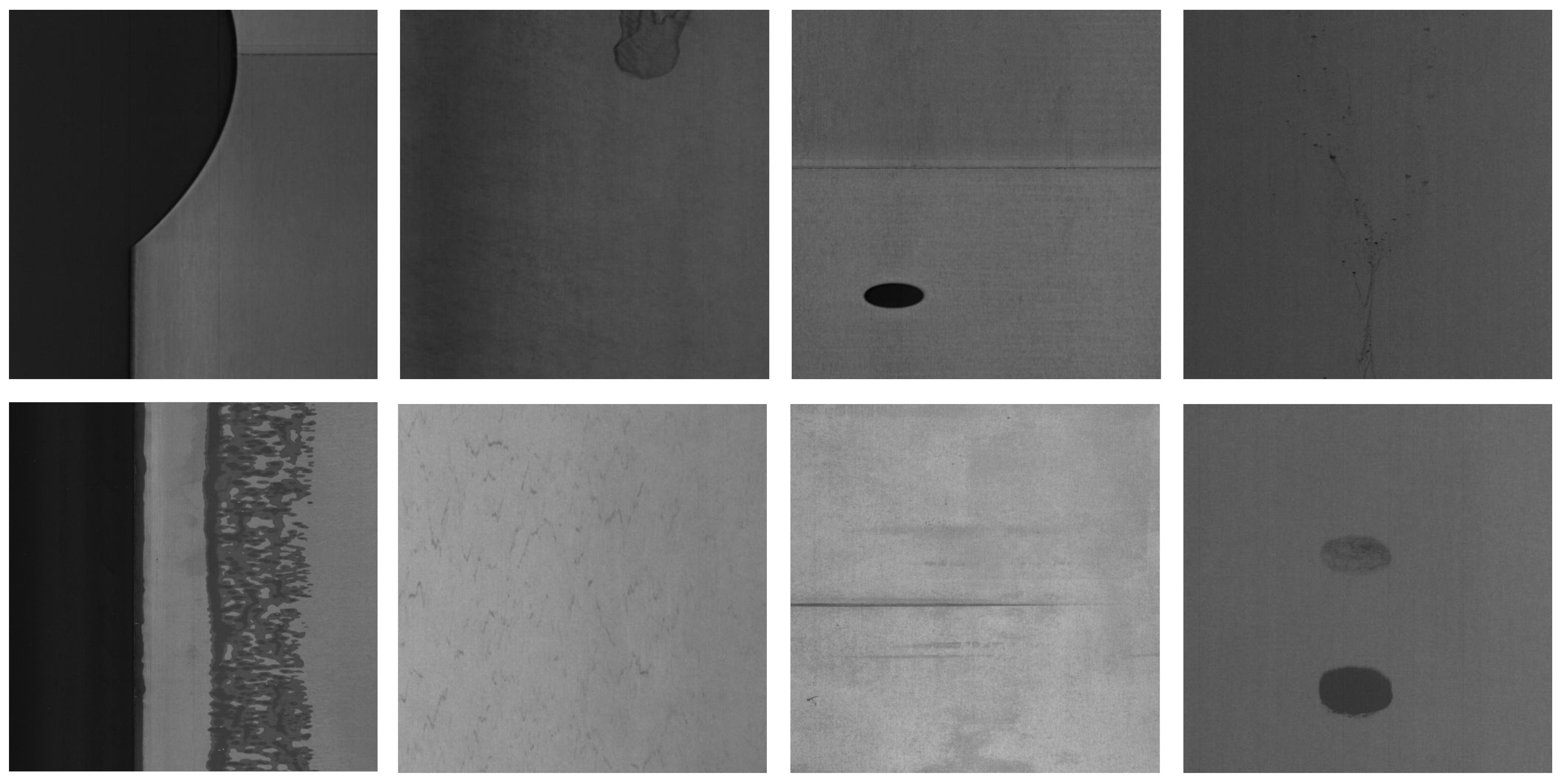
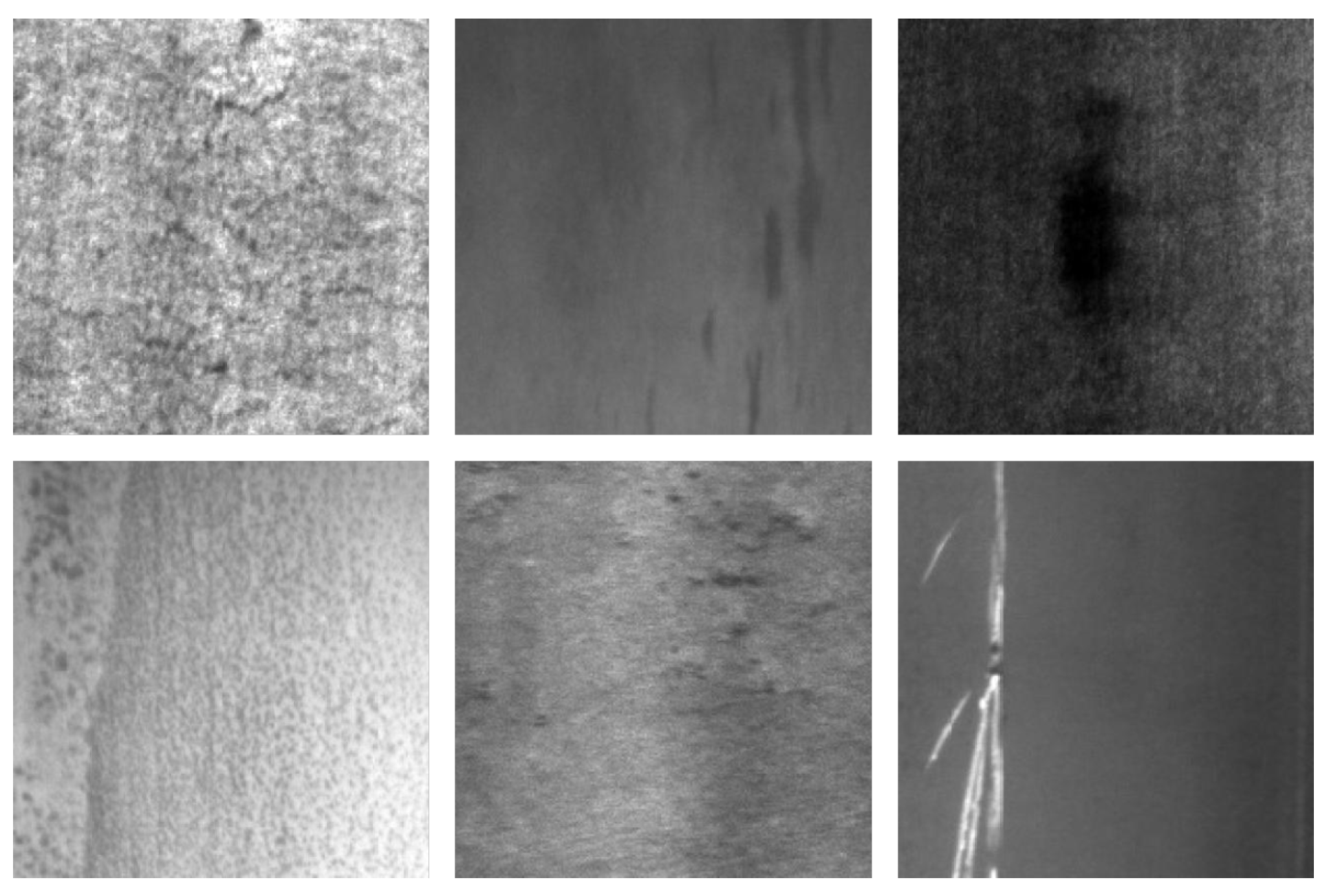
In defect detection tasks, defect images differ significantly from traditional object detection images. Metal defect images exhibit large variations in scale, including extremely small defect samples, and some defect categories have blurry edges, making accurate recognition and localization a major challenge. To address these issues, this study proposes an edge-enhanced feature fusion (EEFF) structure to solve the aforementioned two problems, with the overall module architecture shown in Figure 4. The EEFF comprises the two following components: the SSFF feature fusion architecture and the EEM (edge enhancement module).

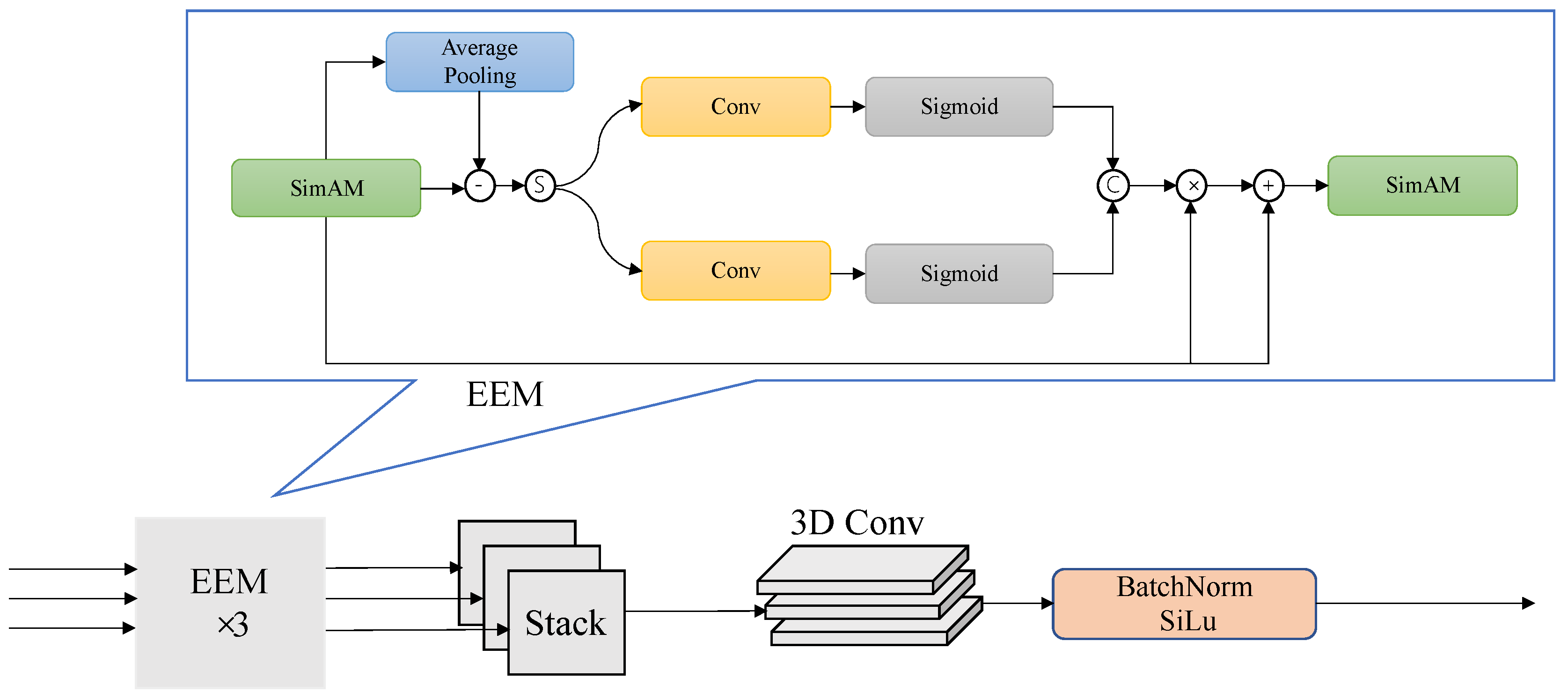
To address the challenge of capturing feature information from numerous small and medium-sized defects in the dataset, we introduce an SSFF module [19] into the algorithm to capture multi-scale feature information. The SSFF module takes three-layer feature maps from the backbone as input. Among these three layers, two are derived from the intermediate backbone layers processed through the DHLC structure, whereas the third layer is obtained by applying dimensionality adjustment via a 1 × 1 convolution to the output of the entire backbone network. Specifically, the method adopts the central layer as a reference framework, leveraging 1 × 1 convolutional filters and nearest-neighbor interpolation to modify channel counts and feature map dimensions in neighboring upper/lower levels, synchronizing them with the central layer while maintaining cross-layer feature alignment consistency. Subsequently, an unsqueeze operation transforms the feature maps into a 4D format (dimensions: depth, height, width, channels), which concatenates them along the depth dimension to form a 3D feature map, preserving multi-scale information. This 3D feature map is further processed using 3D convolutions, 3D batch normalization, and Leaky ReLU activation to effectively capture multi-scale defect target information.

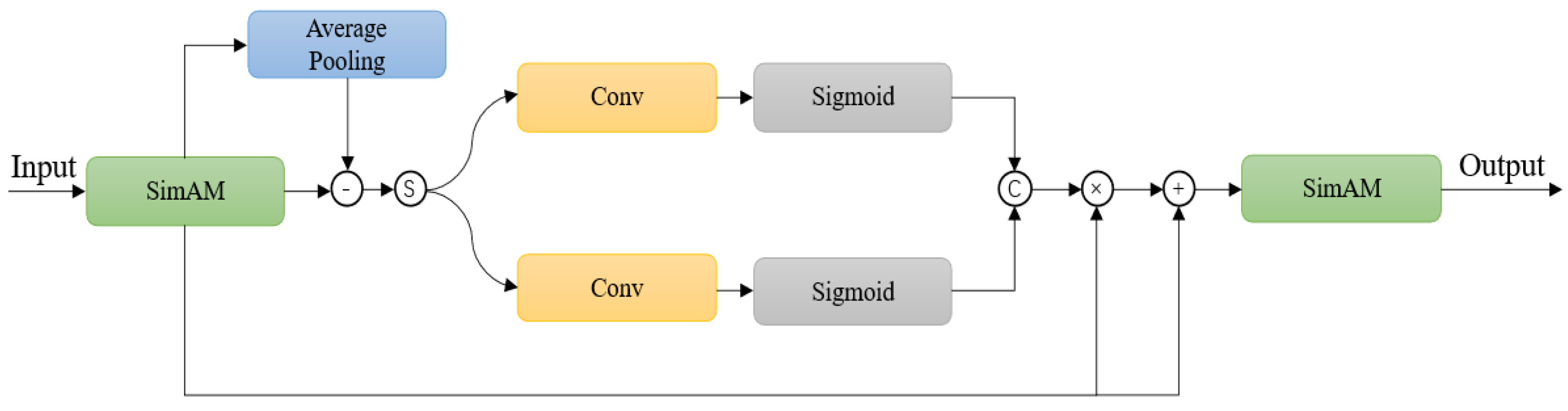
To address the issue of blurred defect edges, we propose an Edge Enhancement Module (EEM) to extract and enhance edge information in features. The overall workflow of the module is illustrated in Figure 5. In the EEM, the first-level input features are initially preprocessed using SimAM attention to identify regions of interest. After SimAM processing, the EEM employs pooling, subtraction, and convolution to extract edge features. Edge features typically manifest as high gradient values. By applying average pooling, the features are smoothed, and then a subtraction operation is performed to subtract the averaged features, thereby highlighting the edge regions. The workflow transitions into a dual-branch structure, employing a 1 × 1 convolutional layer fused with a sigmoid activator to amplify edge feature clarity and prominence. Subsequent refinement occurs via element-wise product and summation mechanisms to intensify these processed signals. Finally, the SimAM attention mechanism is reapplied to focus on critical regions, yielding the refined output feature ${\widehat{X}}_e^t$. The overall workflow of the EEM module is as follows:

$$\begin{array}{c}\widehat{X}=\mathrm{SimAM}\left(X_i\right)\end{array}$$

(2)

$$\begin{array}{c}{X}_e^t=Concat(\sigma ·Con{v}_{1\times 1}\left(Split(\widehat{X}-AP\left(\widehat{X}\right))\right))\times \widehat{X}+\widehat{X}\end{array}$$

(3)

$$\begin{array}{c}{\widehat{X}}_e^t=\mathrm{SimAM}\left(X_e^t\right)\end{array}$$

(4)

where $Con{v}_{1\times 1}$ stands for the 1 × 1 convolution; $AP$ for the average pool; $\sigma$ for the activation function of the sigmoid. Unlike other edge feature extraction methods (e.g., TAFFNet), our method explicitly extracts edge gradients through SimAM-guided pooling-subtraction operations and dual-branch amplification, enabling precise localization of blurred defect contours.

3.5. Focal-MPDIoU Loss

To enhance the model’s training accuracy and convergence speed, this section proposes a novel regression loss. The overall loss function is defined in Equation (5). Where $L_{Focal-MPDIoU}$ represents the proposed bounding box regression loss, and $L_{cls}$ retains the original uncertainty-minimization selection algorithm from RT-DETR. Here, $\widehat{y}$ and y denote the predicted and ground truth values, respectively, while $\{\widehat{b},\widehat{c}\}$ and $\{b,c\}$ correspond to the predicted and ground truth bounding box coordinates and class labels.

$$L\left(\widehat{x},\widehat{y},y\right)=L_{Focal-MPDIoU}\left(\widehat{b},b\right)+L_{cls}\left(U\left(\widehat{x},\widehat{c},c\right)\right)$$

(5)

The cross-entropy loss (CEL) is widely used in classification tasks, and its formulation is defined in Equation (6), where p denotes the predicted probabilities and Y represents the ground truth labels. Since the ground truth values $v_i$ are binary (either 0 or 1), Equation (6) can be simplified to Equation (7).

$$L_{CEL}(P,Y)=-\sum _{i=1}^n{y}_{i}log(p_i)$$

(6)

$$L_{CEL}\left(P,Y\right)=-log\left(p_t\right),p_t=\left\{\begin{array}{c}p\\ 1-p\end{array}\begin{array}{c},y=1\\ ,y=0\end{array}\right.$$

(7)

During model training, if there is an imbalance between positive and negative samples, the model tends to focus excessively on negative samples. Since negative samples (typically background images) belong to easy-to-classify categories, the training process can become dominated by these easily classifiable negative samples, adversely affecting the model’s convergence performance. To address this issue, Lin et al. [20] proposed a novel loss function called focal loss, as shown in Equation (8).

$$L_{FL}=-{\left(1-p_t\right)}^{\gamma }log\left(p_t\right)$$

(8)

By examining Equations (8), it can be observed that focal loss introduces a penalty term ${(1-p_t)}^{\gamma }$ compared to the traditional cross-entropy loss, where the factor $\gamma >0$ ensures the penalty term ${(1-p_t)}^{\gamma }$ is always positive. Consequently, $L_{FL}\le L_{CEL}$. However, the difference of $L_{FL}-L_{CEL}$ becomes larger when $p_t$ is higher and smaller when $p_t$ is lower. This indicates that focal loss prioritizes predictions with higher $p_t$ values more than the original cross-entropy loss (CEL), enabling the model to achieve better performance on harder-to-classify samples. Currently, in classification tasks, focal loss has demonstrated exceptional capability in handling imbalanced datasets.

When using the traditional Intersection over Union (IoU) as a loss function, it suffers from several limitations. For instance, the loss becomes zero when bounding boxes do not overlap, which halts training progress; moreover, it fails to distinguish between different overlap scenarios when IoU values are identical. To address these issues, researchers have proposed improved variants such as GIoU [21], DIoU [22], and CIoU [23]. However, these methods still exhibit significant limitations when handling cases where bounding boxes partially overlap and have aspect ratios similar to the ground truth boxes. To optimize performance in such scenarios, this work adopts the MPDIoU method proposed by Ma et al. [24]. In essence, MPDIoU enhances IoU by introducing an optimization term that reduces the IoU value through the incorporation of distances between the top-left and bottom-right corners of the predicted and ground truth bounding boxes. A detailed formulation is provided in Equation (9). By leveraging $MPDIoU$, the method effectively mitigates the occurrence of overlapping regression boxes with similar characteristics. Here, ($x_1^A,y_1^A$), ($x_2^A,y_2^A$) denote the top-left and bottom-right point coordinates of A and ($x_1^B,y_1^B$), ($x_2^B,y_2^B$) denote the similar point coordinates of B.

$$\left\{\begin{array}{c}{d}_1^2={\left(x_1^B-x_1^A\right)}^2+{\left(y_1^B-y_1^A\right)}^2\\ d_2^2={\left(x_2^B-x_2^A\right)}^2+{\left(y_2^B-y_2^A\right)}^2\\ MPDIoU=IoU-{\displaystyle \frac{d_1^2+d_2^2}{w^2+h^2}}\end{array}\right.$$

(9)

To achieve higher training precision, this study draws inspiration from the loss function design of Zhang et al. [25], integrating $MPDIoU$ with focal loss to propose the Focal-MPDIoU loss (F-MPDIoU loss). During model training, the number of negative samples (background regions) in predictions significantly outweighs positive samples (target objects), resulting in a large proportion of low-quality, low-IoU regression outcomes. These suboptimal predictions hinder the effective minimization of the loss function. To address this issue, we enhance the original MPDIoU by incorporating insights from focal loss. As illustrated in Equation (8), focal loss introduces an adaptive scaling factor ${(1-p_t)}^{\gamma }$ to balance the contribution of positive and negative samples during loss computation. Building on this principle, we augment $MPDIoU$ with a penalty term $Io{U}^{\gamma }$. The complete formulation of Focal-MPDIoU loss is provided in Equation (10).

$$L_{FMPDIoU}=Io{U}^{\gamma }\left(1-MPDIoU\right)$$

(10)

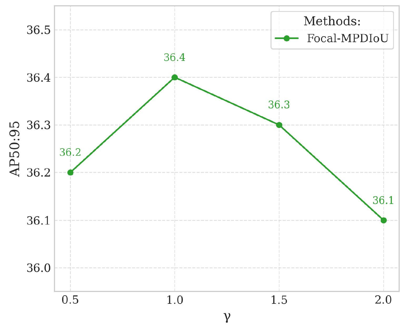
Here, $\gamma$ serves as the penalty term control factor, set to 0.5 in experiments. When the predicted bounding box has a very small IoU value (indicating low confidence in the sample, which is likely a negative instance), the term $Io{U}^{\gamma }$ approaches zero. This mechanism effectively reduces training oscillations caused by low-quality samples and achieves balanced weighting between positive and negative samples. Here, low-quality samples refer to anchor boxes or predicted boxes that exhibit minimal overlap with ground truth target boxes (e.g., very low IoU values) and contribute little meaningful information to model training.

4. Analysis of Experimental Results

4.1. Datasets

During actual production processes, different production lines may have varying steel defect samples. To ensure the generalization and robustness of our method in steel defect detection tasks, we evaluate the performance of MESC-DETR using publicly available steel surface defect datasets. These two datasets are GC10-DET proposed by Tianjin University and NEU-DET proposed by Northeastern University [26,27].

GC10-DET is a steel strip surface defect detection dataset containing 2294 images with ten defect categories. Sample examples in GC10-DET are shown in Figure 6, where the images have been cropped and enlarged for visualization.

Figure 7 illustrates the class distribution and defect scales of the samples. Analysis reveals that the GC10-DET dataset exhibits a class-imbalanced distribution, while steel surface defects across different categories demonstrate significant variations in scale.

NEU-DET is a surface inspection dataset for hot-rolled steel, containing a total of 1800 images. The NEU-DET dataset is categorized into six types of defect images, as follows: crazing, inclusion, patches, pitted surface, rolled-in scale, and scratches. Figure 8 shows the examples of the NEU-DET dataset.

4.2. Experiment Setup

The experiments in this chapter were conducted on a Linux deep learning server. The deep learning server utilizes an Xeon(R) Gold 5222 CPU and RTX 3090 GPU, with experiments performed under the Ubuntu operating system. The programming language primarily utilized Python 3.9, and the software framework employed PyTorch 2.1. The parameter settings are shown in

Table 1. Experimental parameters.

Parameters	Value
Learning rate	0.01
Batch Size	8
Epochs	400
Workers	8
Optimization algorithm	SGD
Momentum	0.937

. To ensure fairness in the comparison, the remaining models in the latter comparison test use the same hyperparameter configuration. In the experiments, two datasets are divided into 7:2:1 training, validation, and test sets, and the Mosaic data enhancement method is used in the training process. For GC10-DET, due to the unbalanced sample distribution, its sparse samples are pre-sampled in the experiments in this chapter, which is used to ensure the overall sample balance and improve the algorithm detection accuracy.

4.3. Experimental Metrics

In this study, we used $mAP$, $Precision$, $Recall$, $F1$, and $FPS$ to evaluate the performance of each model. The formulas for $Precision(P)$ and $Recall(R)$ are as follows:

$$Precision\left(P\right)={\displaystyle \frac{TP}{TP+FP}}$$

(11)

$$Recall\left(R\right)={\displaystyle \frac{TP}{TP+FN}}$$

(12)

where $TP$ (true positive) denotes correct predictions of positive instances, $FP$ (false positive) indicates incorrect predictions of positive instances, $TN$ (true negative) represents correct predictions of negative instances, and $FN$ (false negative) signifies incorrect predictions of negative instances.

Precision (P) and recall (R) represent the model’s performance in terms of accuracy and completeness, respectively. To comprehensively evaluate the model’s performance, precision–recall (PR) values under different confidence thresholds are plotted as a curve. The area under this curve corresponds to the average precision ($AP$) value. The mean average precision ($mAP$) denotes the average precision values across all categories. As the key metric in the experiments of this chapter, mAP effectively reflects the model’s overall performance. The formula for mAP is shown as follows:

$$AP={\int }_0^{1}PdR$$

(13)

$$mAP={\displaystyle \frac{1}{n}}\sum _{i=1}nAP$$

(14)

In defect detection tasks, both recall and precision performance are equally crucial. Therefore, this study also employs the $F1$ score as an additional performance metric. The $F1$ score represents the harmonic mean of precision and recall, effectively balancing these two metrics. The formula for the $F1$ score is expressed in Equation (15):

$$F1=2·{\displaystyle \frac{P·R}{P+R}}$$

(15)

In defect object detection, $FPS$ (frames per second) measures how many images or video frames a model can process and analyze per second. The formula for $FPS$ is shown as follows:

$$FPS={\displaystyle \frac{frameNum}{elapsedTime}}$$

(16)

4.4. Experiment Analysis

4.4.1. Comparison Experiment of Backbone

To validate the distinctiveness of the proposed Composite-ConvNeXt architecture, this study conducts comparative analyses of multiple backbone networks (

Table 2. Comparison experiment of different backbones.

Backbone	${\mathit{AP}}_{50:95}$ (%)	${\mathit{AP}}_{50}$ (%)	FPS (Frame/s)
ResNet-50	33.5	64.7	45.3
ResNet-101	34.1	65.1	37.8
HGNetV2 (l)	32.8	63.2	46.1
HGNetV2 (x)	33.0	63.8	39.1
MobileNetV4	30.9	61.8	52.1
CSWin-T	35.5	67.1	32.1
ConvNeXtV1	31.5	66.8	38.5
ConvNeXtV2	34.5	67.3	39.2

). Compared with ResNet-50, ResNet-101, and HGNetV2 employed in the original RT-DETR, ConvNeXtV2 demonstrates superior performance across all metrics, confirming its enhanced feature extraction capability for defect detection. Experimental comparisons reveal that MobileNetV4 [28] underperforms due to its lightweight design compromises, while CSWin-T [29], though achieving better $A{P}_{50:95}$ scores, shows inferior $A{P}_{50}$ performance and less compact architecture compared to ConvNeXtV2. The streamlined design of ConvNeXtV2 proves more advantageous for practical deployment. We can see that the use of ConvNeXt allows the algorithm to achieve a balance between accuracy and speed. While improving backbone accuracy, it prevents the significant speed degradation typically associated with using large backbone architectures.

Regarding DHLC structure optimization, experiments with varying stacking configurations (

Table 3. Comparison experiment of DHLC connections.

The Number of DHLC Connections	${\mathit{AP}}_{50:95}$ (%)	${\mathit{AP}}_{50}$ (%)	FPS (Frame/s)
1	34.5	67.3	39.2
2	35.1	68.1	33.8
3	34.5	68.3	30.2
4	35.1	68.1	28.4
5	35.3	67.6	27.1

) demonstrate that a dual-backbone architecture effectively enhances feature extraction while maintaining computational efficiency. Excessive stacking beyond three layers introduces parameter redundancy and overfitting risks. It is clear to see that after using multiple backbone network overlays, the speed of the algorithm drops significantly, which is detrimental to our deployment on the production line. Consequently, the dual-backbone design is adopted to balance detection accuracy with computational overhead, ensuring controlled algorithmic complexity.

4.4.2. Comparison Experiment of Loss Function

To validate the effectiveness of the proposed loss function, this study conducts comparative experiments using the enhanced RT-DETR baseline model with C-ConvNeXt and EEFF modules (

Table 4. Comparison experiment of loss functions.

Loss	${\mathit{AP}}_{50:95}$ (%)	${\mathit{AP}}_{50}$ (%)
IoU	34.5	67.3
EIoU	35.2	67.8
CIoU	35.1	66.5
GIoU	34.8	70.2
MPDIoU	36.2	69.8
Focal-MPDIoU	36.4	71.9

). Experimental results demonstrate that GIoU achieves optimal $A{P}_{50}$ performance without focal loss integration but suffers a significant drop in $A{P}_{50:95}$ performance, confirming MPDIoU’s superior suitability for defect detection tasks. The proposed Focal-MPDIoU regression loss, incorporating focal loss penalty terms, achieves balanced optimization with final $A{P}_{50:95}$ and $A{P}_{50}$ scores reaching 36.4% and 71.9% respectively, indicating comprehensive performance enhancement.

We also evaluate the $\gamma$ parameter in the employed methodology. A larger $\gamma$ value exhibits a stronger suppression effect on hard samples but slows down the convergence speed. As shown in Figure 9, we find that setting gamma to 0.5 achieves the best performance, which is consequently adopted as the default value in our loss function.

4.4.3. Ablation Experiment

Ablation study, a methodology for validating model performance, is widely adopted in computer vision to analyze and enhance deep learning architectures through systematic component removal. This section conducts comprehensive ablation experiments on the GC10-DET dataset to evaluate the proposed modules: Composite-ConvNeXt (C-ConvNeXt) backbone, edge-enhanced feature fusion (EEFF) structure, and improved F-MPDIoU loss function. The experimental outcomes in

Table 5. Ablation experiment on the GC10-DET dataset.

Method	${\mathit{AP}}_{50:95}$ (%)	${\mathit{AP}}_{50}$ (%)	${\mathit{AP}}_{\mathit{S}}$ (%)
RT-DETR	33.5	64.7	29.6
+ConvNeXt	34.5	67.3	30.1
+C-ConvNeXt	35.1	68.1	30.2
+C-ConvNeXt+SSFF	35.2	68.4	31.0
+C-ConvNeXt+SSFF (without 3D Conv)	34.9	67.5	30.6
+C-ConvNeXt+SSFF+EEM	35.4	69.9	31.2
+C-ConvNeXt+SSFF+EEM (without pooling/differencing)	34.8	69.1	31.0
MESC-DETR	36.4	71.9	31.0

demonstrate progressive performance improvements from each module. The C-ConvNeXt backbone enhances defect feature extraction, elevating $A{P}_{50}$ from 64.7% to 68.1% and $A{P}_{50:95}$ from 33.5% to 35.1%. The EEFF module strengthens multi-scale detection and edge recognition, further increasing $A{P}_{50}$ to 69.9%. Meanwhile, it can be seen that the SSFF module is of great help for small object detection. With the aid of the SSFF module, the algorithm has achieved a significant improvement in the $A{P}_S$ metric. Additionally, the algorithm’s performance has also been enhanced by leveraging the edge extraction function of the EEM module, and the experiment on the differential component demonstrates this point. Finally, the F-MPDIoU loss achieves optimal performance with $A{P}_{50}$ of 71.9% and $A{P}_{50:95}$ of 36.4%, confirming the cumulative effectiveness of these architectural innovations.

4.4.4. Visual Qualitative Analysis Experiment

This study employs comparative visualization diagrams to intuitively demonstrate the performance improvements of MESC-DETR over the original RT-DETR. Figure 10 presents the detection results of the enhanced RT-DETR algorithm on the GC10-DET dataset, revealing that the modified algorithm achieves precise defect category identification and accurate localization of defect regions on metal surface materials. The visual comparisons distinctly illustrate the superior performance of the proposed method compared to its baseline counterpart. Figure 10a demonstrates the “silk_spot” category characterized by blurred object features and large occupied image areas. The MESC-DETR exhibits effective recognition of edge-blurred objects with accurate boundary delineation and the absence of overlapping bounding boxes, highlighting the efficacy of the EEM module. Figure 10b primarily showcases “inclusion” defects distinguished by their small size and dense distribution. The MESC-DETR demonstrates superior detection capabilities compared to the RT-DETR algorithm, enabling more accurate identification of multiple small defects. However, it exhibits erroneous overlapping bounding boxes not present in RT-DETR detection results, indicating an area requiring future improvement. Figure 10c contains multiple defect categories, where MESC-DETR successfully identifies “rolled-pit” defects undetected by the original RT-DETR algorithm. Despite relatively low confidence scores, this indicates that the detection algorithm possesses stronger capabilities in identifying such blurred objects compared to the original algorithm. Figure 10d,e present targets of varying scales. While MESC-DETR demonstrates comparable performance to RT-DETR in large-scale object detection, it exhibits exceptional small-target detection capabilities, effectively validating the outstanding performance of the multi-scale fusion architecture within the algorithm.

Additionally, this study employs Grad-CAM++ [30] to generate feature visualization maps. As illustrated in Figure 11, the activation patterns of MESC-DETR exhibit concentrated activation peaks on small targets, demonstrating enhanced multi-scale feature perception capabilities. In edge-obscured defect cases, the feature maps show pronounced aggregation of high-intensity responses along boundary regions, evidencing superior edge-aware feature extraction. These visualizations provide intuitive validation of the algorithm’s performance improvements through quantitative spatial activation analysis.

4.4.5. Model Performance Comparison

The experimental results of the MESC-DETR algorithm on the steel surface dataset GC10-DET are presented in

Table 6. Model performances on GC10-DET dataset.

	RT-DETR		MESC-DETR
Class	${\mathit{AP}}_{\mathbf{50}:\mathbf{95}}$ (%)	${\mathit{AP}}_{\mathbf{50}}$ (%)	${\mathit{AP}}_{\mathbf{50}:\mathbf{95}}$ (%)	${\mathit{AP}}_{\mathbf{50}}$ (%)
Crease	22.5	53.8	27.5	66.8
Crescent gap	63.3	90.5	55.3	91.5
Inclusion	7.8	24.4	9.5	33.3
Oil spot	32.5	65.8	31.5	71.9
Punching hole	56.2	93.1	58.4	97.7
Rolled pit	14.8	33.1	15.5	32.5
Silk spot	21.5	49.8	28.5	64.2
Waist folding	33.1	77.8	44.8	91.1
Water spot	36.6	64.4	42.0	73.8
Welding line	46.6	94.6	51.2	96.5
mAP	33.5	64.7	36.4	71.9

. It is observed that the enhanced MESC-DETR demonstrates significant performance improvements over the original RT-DETR on the GC10-DET dataset. Regarding the $A{P}_{50}$ metric, all defect categories exhibit enhancements except for indentation. For the more challenging $A{P}_{50:95}$ metric, improvements are achieved across all categories except crescent gap and oil spot. The proposed algorithm elevates the $A{P}_{50}$ score from 64.7% to 71.9% and increases the $A{P}_{50:95}$ value from 33.5% to 36.4%, demonstrating substantial improvements over the original baseline algorithm in steel surface defect detection.

This study conducts a comprehensive comparative analysis between the proposed method and several prominent algorithms, with optimal results highlighted in boldface as shown in

Table 7. Comparison with different methods on the GC10-DET dataset.

Method	${\mathit{AP}}_{50:95}$ (%)	${\mathit{AP}}_{50}$ (%)	${\mathit{AP}}_{\mathit{s}}$ (%)	${\mathit{AP}}_{\mathit{M}}$ (%)	${\mathit{AP}}_{\mathit{L}}$ (%)	$\mathit{F}\mathbf{1}$ (%)	FPS (Frame/s)
Faster R-CNN [31]	32.5	63.4	27.3	35.3	32.1	68.1	23.1
Cascade R-CNN [5]	33.5	66.1	30.5	25.2	32.5	66.2	16.2
YOLOv5s	32.1	65.2	27.1	28.5	31.2	65.2	132.9
YOLOv8s	34.5	66.1	30.1	31.1	32.2	66.9	105.1
YOLOv11s	31.3	60.6	26.4	32.4	30.3	66.4	92.1
RetinaNet [20]	34.1	68.2	28.1	35.1	32.1	69.5	45.2
FCOS [33]	32.1	66.2	26.4	31.4	31.5	58.2	25.3
VarifocalNet [32]	30.2	64.5	25.1	30.4	26.5	73.1	24.1
Deformable DETR [7]	33.9	66.3	28.5	33.0	29.5	72.8	27.5
RT-DETR	33.5	64.7	29.6	32.1	30.5	68.2	45.3
MESC-DETR (ours)	36.4	71.9	31.0	28.2	33.5	75.1	33.8

. The experimental results demonstrate that the proposed algorithm achieves state-of-the-art performance across all metrics except $A{P}_M$ on the GC10-DET dataset, significantly outperforming other mainstream object detection approaches. These findings substantiate the exceptional capability of our MESC-DETR framework in defect detection applications. To ensure fair comparison, all methods were implemented using their official default hyperparameter settings, trained until network convergence, and subjected to identical dataset preprocessing procedures. The benchmarked algorithms include: Faster R-CNN [31], Cascade R-CNN [5], YOLOv5, YOLOv8, YOLOv11, RetinaNet [20], VarifocalNet [32], FCOS [33], and Deformable DETR [7].

4.4.6. Versatility and Robustness Verification Experiments

We also conducted generalization experiments on the NEU-DET dataset, demonstrating that MESC-DETR successfully identifies defective samples across all classes in the NEU-DET benchmark. Compared with RT-DETR, MESC-DETR exhibits enhanced detection accuracy. Figure 12 shows the detection result of NEU-DET. Notably, it successfully detected targets in scale-type defects that were missed by RT-DETR. Furthermore, MESC-DETR effectively eliminated the duplicate bounding box artifacts observed in RT-DETR’s detection of oxide scale defects. For crack-type defect detection, MESC-DETR achieved superior confidence scores and more precise localization accuracy while maintaining equivalent detection capability to RT-DETR.

The detailed detection results for NEU-DET are presented in

Table 8. Versatility and robustness verification experiments on the NEU-DET dataset.

	RT-DETR		MESC-DETR
Class	${\mathit{AP}}_{\mathbf{50}:\mathbf{95}}$ (%)	${\mathit{AP}}_{\mathbf{50}}$ (%)	${\mathit{AP}}_{\mathbf{50}:\mathbf{95}}$ (%)	${\mathit{AP}}_{\mathbf{50}}$ (%)
Crazing	22.5	51.8	31.2	61.2
Inclusion	41.7	81.5	35.6	81.1
Patches	70.2	90.5	73.2	91.5
Pitted surface	68.1	90.0	71.2	89.6
Rolled-in scale	25.1	59.4	24.8	64.5
scratches	50.2	86.5	50.5	93.9
mAP	46.3	76.6	47.8	80.3

. The results demonstrate that all defect categories exhibited improvements in $A{P}_{50}$ metrics with the exception of inclusions and pitted surfaces, indicating the superior performance of the proposed algorithm on the NEU-DET dataset. Furthermore, enhancements in $A{P}_{50:95}$ values were observed across all categories except for inclusions and rolled-in scale. The algorithm achieved comprehensive performance improvements, elevating the $A{P}_{50}$ metric from 76.6% to 80.3% and increasing the $A{P}_{50:95}$ value from 46.3% to 47.8% for the NEU-DET dataset.

5. Conclusions and Discussions

Overall, this study proposes a novel high-precision algorithm named MESC-DETR for steel surface defect detection. Specifically, the RT-DETR framework was selected as the baseline model and underwent targeted modifications to optimize its performance for steel defect detection tasks. First, we analyzed the limitations of the original backbone network in defect detection applications and replaced it with ConvNeXtV2, a more robust architecture. Subsequently, a Composite-ConvNeXt backbone was constructed through DHLC (dual homogeneous layer composition) integration, combining two identical ConvNeXtV2 networks. To address challenges, including small targets and blurred edges in the dataset, an SSFF structure was implemented along with a specially designed bypass edge enhancement module (EEM). Furthermore, the proposed Focal-MPDIoU loss function was employed to accelerate model convergence while improving defect localization accuracy. Experimental results demonstrate that MESC-DETR achieves $mA{P}_{50}$ and $mAP$ of 36.4% and 71.9%, respectively, on the GC10-DET dataset, representing improvements of 2.9% and 7.2% over the baseline RT-DETR. Additionally, it shows performance enhancements of 3.7% in $mA{P}_{50}$ and 1.5% in $A{P}_{50:95}$ on the NEU-DET benchmark, confirming its superior generalization capability across various metallic surface defects. However, this paper still has areas that require further improvement. For example, the study sacrifices some algorithmic speed to enhance the accuracy of the RT-DETR algorithm in defect detection, which poses certain challenges when dealing with high-speed production scenarios. In subsequent research, we will further optimize the speed of related algorithms to ensure that their accuracy improvements are achieved while maintaining or even improving their speed. Additionally, we will focus on the deployment performance of the algorithm on edge devices to better align with the requirements of industrial production lines.