Modeling and Analysis in the Industrial Internet with Dual Delay and Nonlinear Infection Rate

Abstract

This study proposes a novel virus propagation model designed explicitly for SCADA(supervisory Control and Data Acquisition) industrial networks. It addresses a critical limitation in existing models applied to the Internet and Industrial Internet of Things (IIoT)—their failure to account for inter-node information exchange processes. The model is inspired by the phenomenon that “immune” nodes in real-world and biological systems inhibit the spread of viruses by exchanging information. This model incorporates isolation strategies to curb virus transmission, considering the uncertainty of vulnerable device behavior. Central to this research are the assumptions of a nonlinear infection rate and dual delays, which better mirror the real-world conditions of industrial control networks. This approach diverges significantly from prior studies that relied on bilinear infection rate assumptions. This study constructed an SMIQR model through theoretical derivation and experimental validation. The model enables nodes to autonomously enhance their defenses after receiving risk information while accounting for the impact of inter-node information exchange. Experiments based on real-world data demonstrated the model’s effectiveness in simulating virus propagation and evaluating defense strategies, overcoming the limitations of traditional bilinear infection rate assumptions. Comparative experiments show that the SMIQR model significantly reduces the number of infected nodes in SCADA industrial networks, demonstrating its superior effectiveness in curbing virus spread. Furthermore, the research proposed dynamic isolation tactics that balance industrial operational continuity, providing SCADA industrial networks with a theoretical framework (incorporating nonlinear infection rates and dual delay characteristics) and practical defense solutions to curb malware spread without disrupting production.

1. Introduction

Supervisory Control and Data Acquisition (SCADA) systems are widely used to monitor and control critical infrastructures such as power, chemicals, water treatment, oil, and gas, ensuring their operational efficiency and safety [1]. However, with the rise in networking and the advent of the 5G era, industrial control systems are no longer isolated and physically secure, making them more vulnerable to cyber threats [2,3].

The basic architecture of a SCADA system consists of multiple levels and components, including field devices, communication networks, data acquisition and control layers, SCADA control centers, data storage and analysis, alarm and event management, and operation and control. Field devices, such as sensors, actuators, programmable logic controllers (PLCs) [4], and remote terminal units (RTUs), act as interfaces between field devices and SCADA systems. PLCs are typically used for automation control, while RTUs are primarily employed for remote monitoring and data transmission. These components work together to monitor, manage, and optimize industrial processes. However, the increasing interconnectivity and complexity of SCADA systems, driven by the industrial Internet, have exposed them to more significant risks of cyberattacks. Malicious viruses often infiltrate the physical layer of RTU nodes through network interfaces, leading to system failures, data breaches, or complete system crashes.

The development of computer virus propagation models has evolved through several stages, with researchers continuously proposing new theories and models to explain and predict virus propagation behavior. Recent advances by Zhang et al. [5] further integrate qualitative differential equations with evolutionary game theory to achieve dynamic threat assessment in modern network environments. In the 1980s, the concept of computer viruses emerged, and scholars introduced simple propagation models such as the SIS model [6,7,8], which assumed that a system could be either infected or uninfected. In the 1990s, inspired by epidemiological models, researchers developed the SIR model [9], which divided computer systems into three states [10] and described the lifecycle of virus propagation. Over time, researchers extended these models to incorporate additional factors such as network topology, propagation routes, and virus variants. For example, the SIRS model [11] introduced a susceptible–infected–recovery–susceptible cycle, allowing systems to become susceptible again after virus removal. Early models often simulated information transmission as direct virus transmission, overlooking the inherent differences between the two, such as information transmission’s memory and delay characteristics. Dodds and Watts [12] studied the effect of limited memory on infection, while Zhao et al. [13] proposed an SVEIR model with time delay and nonlinear incidence, deriving explicit formulas for determining the direction of Hopf bifurcation and the stability of periodic solutions. Safar proposed the SEIQP model [14] to study worm insider threats. Sulaiman et al. enhanced this model to SEIQV [15], incorporating worm internal threats and validating its effectiveness through neural networks and optimization algorithms. Tang et al. [16] introduced the SLBRS model, which used security entropy to study virus transmission security. At the same time, Zhang and Gan [17] proposed an improved SLBR model to analyze the combined effects of infected external computers and removable storage media on virus transmission. Subsequent research on multi-objective optimization algorithms also contributed to the optimization strategies for virus propagation models [18]. Foundational studies by Shen et al. [19] established differential game-theoretic frameworks for malware containment in wireless sensor networks. Matta et al. [20] innovatively adapted birth–death–immigration processes for modeling cyber threats.

Within SCADA industrial network environments, propagation modeling research primarily aims to simulate malware dissemination patterns, enabling systematic analysis of potential security vulnerabilities through computational epidemiological approaches. Carcano et al. [21] analyzed the transition of SCADA systems from safe to dangerous states by examining data flows generated by network attacks, improving intrusion detection systems (IDS) accuracy. Sheng et al. [22] proposed a mathematical model to study industrial virus transmission in SCADA systems, combining defense measures with intelligent honeynets to offer comprehensive protection strategies. Wang et al. studied the Stuxnet malware [23], which caused significant damage to nuclear power plant SCADA systems, and provided patch codes through static analysis [24]. In addition to these traditional research directions, notable advancements have been made in exploring novel theoretical frameworks and leveraging emerging technologies. Specifically, Srivastava et al. [25] developed cyber-immunity mechanisms inspired by infectious disease ecology. He et al. [26] proposed an immune knowledge-driven propagation model specifically optimized for SCADA virus dynamics. Meanwhile, breakthroughs in machine learning, particularly the cognitive-driven label transition methods by Zhang et al. [27] and their part-aware correlation networks [28], have enabled more precise estimation of system state transitions in data-scarce SCADA environments. Attacks on components such as PLCs, RTUs, servers, and databases have severely harmed industrial control systems. RTUs, critical for remote data acquisition and equipment monitoring, are particularly vulnerable. For instance, the 2015 cyberattack on Ukraine’s power infrastructure involved infected RTUs manipulating switchgear, leading to widespread power outages [29]. Such attacks can disrupt industrial processes, causing substantial economic losses and posing threats to security, privacy, and public safety [30]. Zhu et al. [31] proposed the SLBR model, highlighting that highly contagious viruses in SCADA systems immediately affect RTU nodes without latency, making them difficult to suppress. Additionally, studies have proposed protective measures [32,33] in technology, personnel, management, and facilities to mitigate virus propagation in SCADA systems [34] and proposed several containment strategies for malware [35,36]

In summary, most studies on virus propagation in the Internet and Industrial IoT have focused on external factors such as propagation paths and situational influences, often neglecting the role of information exchange between nodes. Inspired by real-world and biological systems, such as rumor propagation dynamics in social networks, risk contagion mitigation in financial markets, traffic flow optimization in urban transportation, and adaptive immune response mechanisms in living organisms, the model can enhance the overall system’s antiviral capability through inter-node information exchange. Taking biological immunology as an example; in this context, during the humoral immune response of cells, T cells, upon recognizing antigens, proliferate and differentiate into effector T cells and memory T cells. Effector T cells release lymphokines, which enhance the immune responses of other cells, thereby amplifying the body’s overall immune reaction. This mechanism can be analogously applied to industrial networks. In such networks, RTU (Remote Terminal Unit) nodes may probabilistically transmit danger signals to uninfected RTU nodes via wired cables, radio transmission, Ethernet, or other communication channels. Thus, infected RTU nodes mimic the release of lymphokines by infected T cells to propagate danger signals, ultimately enhancing the collective antiviral capacity of the RTU network. This delivery mechanism fundamentally differs from the classical SIR/SIRS epidemiology model. The classical model in which nodes enter the infected state immediately after a successful attack ignores some of the defense capabilities that nodes may have in real industrial environments. The existence of M alters this scenario. Instead of passively succumbing to infection when facing threats, nodes in the network can obtain early-warning information through M and actively adjust their defense strategies. By transmitting danger signals via S, other nodes can activate their defense mechanisms in advance, enhancing their resilience against viruses or malicious attacks. Different nodes can activate the defense mechanism through the danger signal transmitted by S in advance to improve their resistance to viruses or malicious attacks. This early defense mechanism significantly reduces the probability of nodes being infected, which substantially enhances the collective antivirus capability of the entire RTU network, effectively guaranteeing the safe and stable operation of the industrial network, as if injecting a strong immunity for the model, making it more robust in the face of complex and changing network threats.

Based on this, this paper introduces a new SCADA industrial virus propagation model, SMIQR, with dual delay and nonlinear infection rate to address the above shortcomings and analyze the system’s impact of these factors.

The proposed model innovatively incorporates three key features. It considers dual delays (infection isolation and immunity loss) to mirror real-world SCADA system behaviors, such as patching and quarantine delays. Unlike traditional models with linear infection rates, it adopts a nonlinear rate to better capture the complex dynamics of malware spread under heavy loads. Additionally, it integrates risk information dissemination, using the “M” state to simulate nodes gaining partial immunity through information exchange. These elements enable a more accurate and comprehensive representation of malware propagation and defense in industrial networks.

The main contributions of this paper are as follows:

(1)

A novel SMIQR virus propagation model is proposed for SCADA industrial systems. This model incorporates node information transfer mechanisms to simulate how nodes strengthen defenses upon receiving danger signals.

(2)

The model introduces a nonlinear infection rate to capture the non-proportional growth of infections under high loads, accounting for network congestion and defense resource constraints.

(3)

The model combines dual delays, namely the infection isolation and immunization loss delays. Through a rigorous mathematical proof analysis, these two delays are analyzed to have an inseparable impact on system stability, showing that their combined effect cannot be ignored and must be considered together in real industrial environments.

(4)

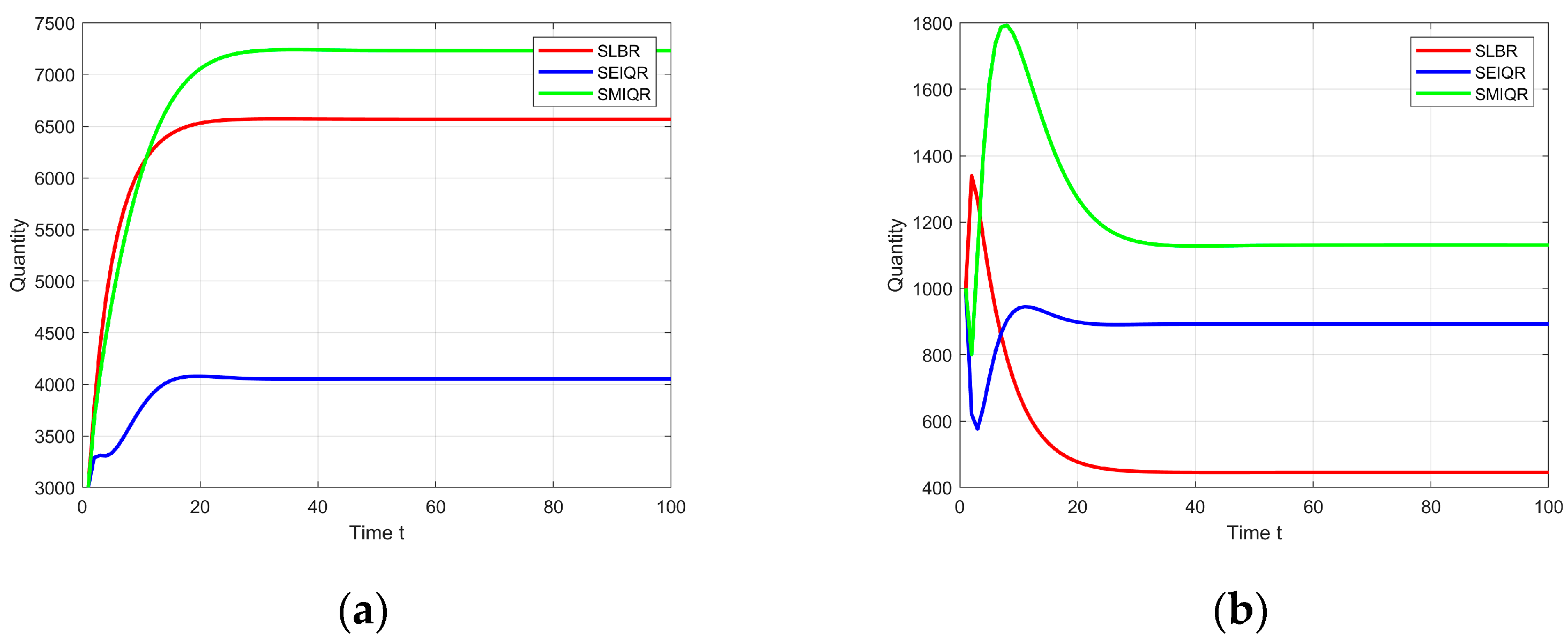
An empirical comparison with the SLBR/SEIQR model validates the effectiveness of the SMIQR model for malware propagation in industrial networks.

(5)

A security defense strategy is developed to balance malware containment with uninterrupted industrial production, leveraging the model’s unique features.

These contributions advance the realism and applicability of cybersecurity modeling in industrial control systems.

The structure of this article is as follows: Section 2 describes the SMIQR model and analyzes its parameters. Section 3 introduces the theoretical derivation of the model. Section 4 conducts numerical simulations to demonstrate the system’s stability under different conditions and examines the impact of dual time delays on the system. Section 5 verifies the model’s effectiveness using a real dataset and analyzes its sensitivity to infection suppression factors. Section 5 is a model comparison experiment to confirm the validity of the SMIQR model. Finally, this article summarizes and proposes security defense strategies to prevent the spread of malicious software without affecting industrial production.

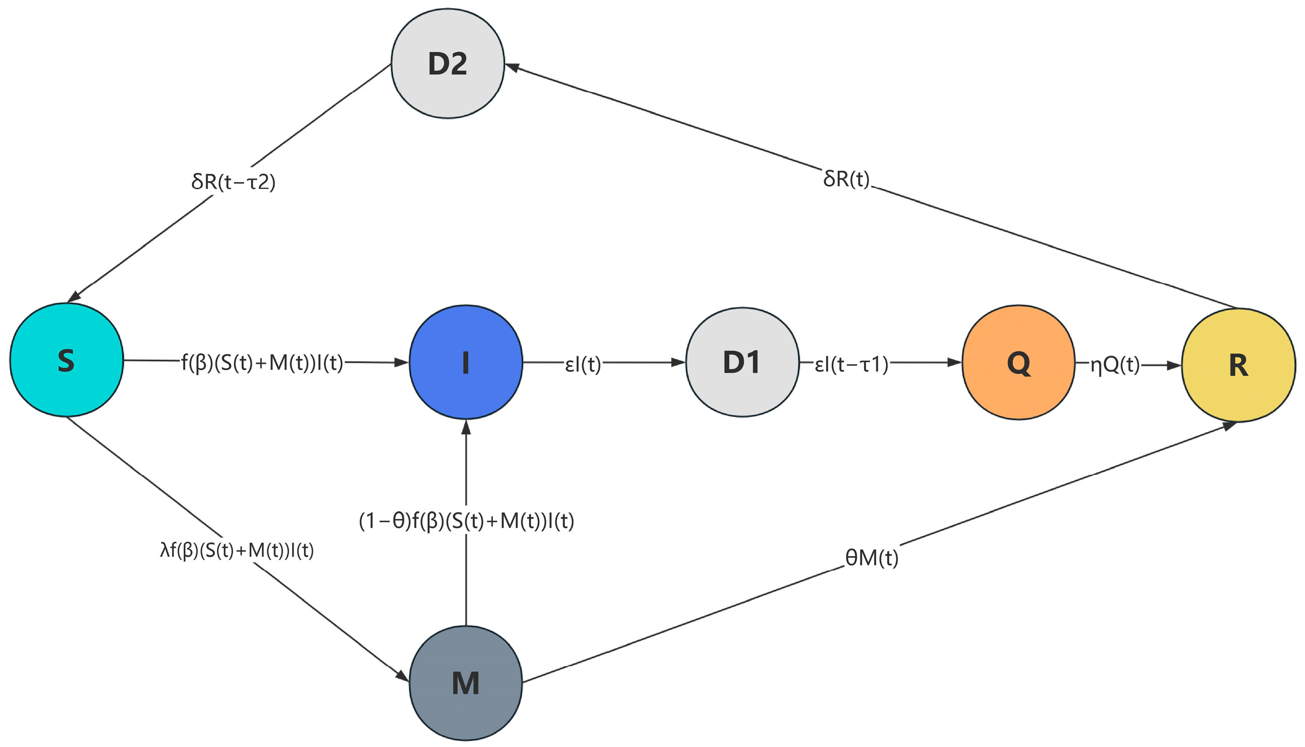
2. Model Formulation

2.1. Model Node Configuration

With the gradual realization of interconnection, integration, and remote monitoring of industrial equipment, the traditional closed network architecture has been gradually broken. SCADA systems have become more complex and highly dependent on network connections. In this new network environment, one of the main risks faced by SCADA systems is the security of their physical layer RTU (Remote Terminal Unit) nodes, which are the core components of SCADA systems and are responsible for collecting data from field devices and transmitting it to the upper control system. They are typically installed at the edge of an industrial facility and connect directly to physical devices, sensors, and actuators for data acquisition, signal forwarding, and field control. As industrial equipment opens up to remote access, RTU nodes are exposed to the public Internet or internal corporate networks, which can be accessed remotely by hackers through the network interface, who can implant malware and execute malicious code, thus leading to significant problems such as data tampering, system damage, and information leakage. To improve the overall immunity of the SCADA system and better characterize the virus propagation of the SCADA industrial network driven by immune information and inspired by the application scenarios in life, we propose an M-node that exchanges information between nodes and thus has a specific immunity. In the propagation model, when a susceptible node is infected, some susceptible nodes, after receiving information from other infected nodes, develop immunity and thus become enhanced immune nodes with antiviral capability. Based on this, we establish the following seven components:

Susceptible state (S): RTUs susceptible to SCADA systems.

Enhanced state (M): RTUs strengthened through danger signal propagation possess inherent defensive capabilities. If such a node successfully resists viral intrusion after receiving danger signals, it transitions directly into an immune RTU state (R). Conversely, if the defensive measures prove ineffective, the node becomes infected (I).

Infected state (I): RTUs in the system that are infected and can propagate viruses

Delayed state 1 (D1): isolation of RTUs that require a certain amount of time, resulting in a time-delayed state from the I state to the Q state.

Quarantine state (Q): RTUs that centrally manage the state of infection to control the spread of viruses.

Immunity state(R): RTUs that have entered the immunity state by restoring normalcy through antivirus software or patching.

Delayed state 2 (D2): The recovery state becomes susceptible again due to a virus update or patch failure in the system. This failure process is not instantaneous, but an inevitable delay leads to the RTU of the delayed state.

2.2. Model Dynamical Equations

In our virus propagation model, the industrial control network is assumed to be homogeneous to ensure approximately uniform node connectivity. This assumption aligns with the operational reality of RTU device layers in industrial scenarios.

The transition diagram between each state of the model is shown in Figure 1 below, and S, M, I, Q, and R represent the number of RTUs in each state at time t, respectively. Our model is based on the following theoretical definition:

(1)

The RTU accesses the SCADA system at a constant rate b, and each state node can leave the system at a constant rate of $\mu$.

(2)

Assuming that each susceptible node is infected at moment t with a nonlinear infection rate ${\displaystyle \frac{\beta }{1+\mathrm{a}\mathrm{I}}}$. Since both S and M nodes are essentially susceptible states, both can be infected by the infected node. Also, since the M state is not easily infected through the message passing of the infected node, there are${\displaystyle \frac{\beta }{1+\mathrm{a}\mathrm{I}}}$ (S + M)I infected S nodes at moment t.

(3)

$\lambda$ denotes the rate at which infected nodes infect messages at time t. The number of infected nodes at time t is ${\displaystyle \frac{\beta }{1+\mathrm{a}\mathrm{I}}}(\mathrm{S}+\mathrm{M})\mathrm{I}$. Then, there are $\lambda {\displaystyle \frac{\beta }{1+\mathrm{a}\mathrm{I}}}(\mathrm{S}+\mathrm{M})\mathrm{I}$ nodes with states from S to M.

(4)

$\theta$ indicates the magnitude of its defense capability in M state; some M state nodes can be directly converted to R immune state, and there are also (1 − $\theta )$M nodes that are converted to I state nodes after receiving the danger information.

(5)

With antivirus or anti-malware tools, there is a $\epsilon$ probability that a virus will be detected and quarantine measures will be taken such that nodes in the infected state of the system will be changed to quarantined nodes.

(6)

$\sigma$ indicates the probability that a node in the quarantine state of the system transitions to the immune state, in which the quarantined computers may be scanned and repaired, the antivirus software is updated, and the system is protected from viruses by eliminating vulnerabilities and enhancing protection mechanisms.

(7)

Viruses may be updated in the process. If security patches are not installed in a timely manner, there is a $\sigma$ probability that an immune node in the system will become susceptible again.

(8)

Due to the system’s time windowing mechanism and the resulting isolation delay, ${\tau }_1$ describes the time from the infected state to the isolated state.

(9)

In the case of virus variants or patch failure within the SCADA system, this process lasts for a specific period, resulting in an immunization delay described by ${\tau }_1$ from the immune state to the susceptible state.

2.3. Modeling Theory

$$\left\{\begin{array}{l}{\displaystyle \frac{dS}{dt}}=b-(\lambda +1)\beta {\displaystyle \frac{1}{1+\mathrm{aI}(t)}}(S(t)+M(t))I(t)+\sigma R(t-\tau 2)-\mu S(t)\\ {\displaystyle \frac{dM}{dt}}=(\lambda +\theta -1)\beta {\displaystyle \frac{1}{1+\mathrm{aI}(t)}}(S(t)+M(t))I(t)-\theta \mathrm{M}(t)-\mu M(t)\\ {\displaystyle \frac{dI}{dt}}=(2-\theta )\beta {\displaystyle \frac{1}{1+\mathrm{aI}(t)}}(S(t)+M(t))I(t)-\epsilon I(t)-\mu I(t)\\ {\displaystyle \frac{d\mathrm{D}1}{dt}}=\epsilon I(t)-\epsilon I(t-\tau 1)-\mu \mathrm{D}1\left(\mathrm{t}\right)\\ {\displaystyle \frac{dQ}{dt}}=\epsilon I(t-\tau 1)-\eta Q(t)-\mu Q(t)\\ {\displaystyle \frac{dR}{dt}}=\eta Q(t)+\theta \mathrm{M}(t)-\sigma R(t)-\mu R(t)\\ {\displaystyle \frac{d\mathrm{D}2}{dt}}=\sigma R(t)-\sigma R(t-\tau 2)-\mu \mathrm{D}2\left(\mathrm{t}\right)\end{array}\right.$$

(1)

The initial conditions are $\mathrm{S}\left(0\right)\ge 0,\mathrm{M}\left(0\right)\ge 0,\mathrm{I}\left(0\right)\ge 0,\mathrm{D}1\left(0\right)\ge 0,\mathrm{Q}\left(0\right)\ge 0,\mathrm{R}\left(0\right)\ge 0,\mathrm{D}2\left(0\right)\ge 0$, all parameters are positive, and Z(t) = (S, M, I, D1, Q, R, D2). Therefore, let the following be established:

$$N_t=S_t+M_t+I_t+D{1}_t+Q+R_t+D{2}_t,$$

(2)

In turn, the following can be obtained:

$$\Omega =\left\{(\right.S,M,I,D1,Q,R,D2)\in R^{+}|0<N_t<b/\left.\mu \right\},$$

(3)

Theorem 1. 

The set$\Omega$ is positively invariant for system (1), which implies that if Z(0)$ϵ\Omega$, then Z(t)$ϵ\Omega$ for all t ≥ 0.

Proof. 

Summing up the differential equations in system (1) above, we obtain the following:

$${\displaystyle \frac{\mathrm{dN}}{\mathrm{dt}}}={\displaystyle \frac{\mathrm{dS}}{\mathrm{st}}}+{\displaystyle \frac{\mathrm{dM}}{\mathrm{dt}}}+{\displaystyle \frac{\mathrm{dI}}{\mathrm{dt}}}+{\displaystyle \frac{\mathrm{dD}1}{\mathrm{dt}}}+{\displaystyle \frac{\mathrm{dQ}}{\mathrm{dt}}}+{\displaystyle \frac{\mathrm{dR}}{\mathrm{dt}}}+{\displaystyle \frac{\mathrm{dD}2}{\mathrm{dt}}}=\mathrm{b}-\mu \mathrm{N},$$

(4)

Let $S_t\left(0\right)\ge 0M_t\left(0\right)\ge 0I_t\left(0\right)\ge 0{D1}_t\left(0\right)\ge 0Q_t\left(0\right)\ge 0R_t\left(0\right)\ge 0{D2}_t\left(0\right)\ge 0$

$$\because {\displaystyle \frac{\mathrm{dN}}{\mathrm{dt}}}=\mathrm{b}-\mu ,$$

(5)

$$\therefore \mathrm{t}\to \infty ,{\mathrm{N}}_{\mathrm{t}}\to {\displaystyle \frac{ \mathrm{b}}{\mu }},$$

(6)

The above proves that the total node value ${\mathrm{N}}_{\mathrm{t}}$ is positively bounded when the values of all nodes are positive.

To prove the non-negativity of the solution of system (1):

Assuming that$S_t{,M}_t,I_t,{D1}_t,Q_t,R_t,{D2}_t$are not always positive, we have the following:

$$\mathrm{k}(\mathrm{t})=\min \left(S_t,M_t,I_t,D{1}_t,Q_t,R_t,D{2}_t\right),$$

(7)

Then, there must be a time as follows:

$$\mathrm{k}(\mathrm{t}1)<0$$

(8)

Since the kinetic equations are all continuous functions, when the above situation occurs, the system must have t = t2, such that the following is established:

$$\mathrm{k}(\mathrm{t}2)=0,$$

(9)

The assumptions are as follows:

$$\mathrm{k}(\mathrm{t}2)={\mathrm{S}}_{\mathrm{t}}(\mathrm{t}2)=0,$$

(10)

These exist when $0\le \mathrm{t}\le \mathrm{t}2,S_t\left(0\right)\ge 0,M_t\left(0\right)\ge 0{,I}_t\left(0\right)\ge 0{,D1}_t,\left(0\right)\ge 0,Q_t\left(0\right)0,R_t\left(0\right)\ge 0,{D2}_t\left(0\right)\ge 0$. Therefore, in system (1), the nonlinear infection rate is set to f(I) for ease of observation, and we obtain the following equation:

$${\displaystyle \frac{\mathrm{dS}}{dt}}\ge -(\lambda +1)\beta \mathrm{f}(\mathrm{I})\left(S+M\right)I-\mu S,$$

(11)

Then, the following can be obtained:

$${\displaystyle \frac{\mathrm{dS}}{\mathrm{S}}}\ge -\left((\lambda +1)\beta \mathrm{f}(\mathrm{I})\left(1+{\displaystyle \frac{M}{\mathrm{S}}}\right)I+\mu \right)\mathrm{dt},$$

(12)

$$\therefore {\displaystyle {\int }_0^{\mathrm{t}2}\frac{\mathrm{dS}}{\mathrm{S}}}\ge -{\displaystyle {\int }_0^{\mathrm{t}2}\left[(\lambda +1)\beta \mathrm{f}(\mathrm{I})\left(1+\frac{\mathrm{M}}{\mathrm{S}}\right)\mathrm{I}+\mu \right]}\mathrm{dt},$$

(13)

In this equation, the change in the number of S nodes depends only on the current number of other nodes. Hence, the following inequality can be obtained:

$$\mathrm{S}(\mathrm{t})\ge {\mathrm{S}}_{\mathrm{t}}(0)\exp [-((\lambda +1)\beta \mathrm{f}(\mathrm{I})(1+{\displaystyle \frac{M}{\mathrm{S}}})\mathrm{I}+\mu )\mathrm{t}],$$

(14)

It is clear that the right-hand side of the above equation is greater than 0; therefore, the equation$\mathrm{k}\left(\mathrm{t}2\right)=$ 0 does not hold.

Thus, the solution of system (1) is positive and bounded, satisfying the following equation:

$$\Omega =\{(\mathrm{S},\mathrm{M},\mathrm{I},\mathrm{D}1,\mathrm{Q},\mathrm{R},\mathrm{D}2)ϵ{\mathrm{R}}^{+}|0<{\mathrm{N}}_{\mathrm{t}}<{\displaystyle \frac{\mathrm{b}}{\mu }}\},$$

(15)

Therefore, Theorem 1 can be proven. □

3. Derivation

The main work in this chapter is to perform a mathematical theoretical analysis of the system (1). The dynamic behavior of the model is determined by the basic regeneration number [37] $R_0$. The value of $R_0$ is directly related to the evolutionary trend of the model. Therefore, in this chapter, the basic regeneration number $R_0$ is solved first, and then the local and global attraction of the virus-free equilibrium and the epidemic equilibrium are solved separately.

3.1. Basic Regeneration Number R₀

In viral transmission modeling, the basic regeneration number, usually denoted by the symbol ${\mathrm{R}}_0$, is a parameter that describes the average number of susceptible individuals to which an individual can spread during its period of infection. It is a significant indicator in epidemiology, reflecting the potential for transmission and the difficulty of controlling an infectious disease.

The basic regeneration number is a key threshold for determining the presence of a virus in a system. In the following, we use a next-generation matrix [38] to calculate the basic regeneration number ${\mathrm{R}}_0$, representing the average number of SCADA nodes infected at some time t during the infection period. Since there are only I infected nodes, both w and v are first-order matrices, as follows:

$$\mathrm{F}=\left[\begin{array}{c}(2-\theta )\beta {\displaystyle \frac{1}{1+\mathrm{aI}}}(\mathrm{S}+\mathrm{M})\mathrm{I}\end{array}\right],\mathrm{V}=[\epsilon \mathrm{I}+\mu \mathrm{I}],$$

(16)

Again, since S and M are essentially susceptible nodes and M can only be converted from S, we do not care about the number of M and S, respectively, but more about their sum. Thus, we compose S and M as follows:

$$\tilde{S}=\mathrm{S}+\mathrm{M},$$

(17)

When E0 = ($\widetilde{{\mathrm{S}}_0},\mathrm{0,0},\mathrm{0,0},\mathrm{0,0}$) and$\widetilde{{\mathrm{S}}_0}$ = b/$\mu$, the F and V matrices can be expressed as follows:

$${\mathrm{F}}^{\prime }=\left[(2-\theta )\beta {\displaystyle \frac{1}{{(1+\mathrm{aI})}^2}}\widetilde{S_0}\right],V^{\prime }=\left[\epsilon +\mu \right],$$

(18)

The basic regeneration number R0 of the model is the following:

$${\mathrm{R}}_0={\displaystyle \frac{(2-\theta )\beta \widetilde{S_0}}{\epsilon +\mu }},$$

(19)

3.2. Equilibrium Point Stability Analysis

In order to solve the equilibrium point of the viral propagation model SMIQR for node information exchange, we assume the following equations in [39,40], if the dynamic model satisfies one of the local asymptotic stability or global asymptotic stability, it will converge to the corresponding equilibrium point starting from a certain point in the space. This section discusses the equilibrium points of virus propagation under the SMIQR model. The steady state of the SMIQR model satisfies the following equations:

$$\left\{\begin{array}{l}b-(\lambda +1)\beta {\displaystyle \frac{1}{1+\mathrm{a}{I}_0^{*}}}\left(S_0^{*}+M_0^{*}\right)I_0^{*}+\sigma R_0^{*}-\mu S_0^{*}=0\\ (\lambda +\theta -1)\beta {\displaystyle \frac{1}{1+\mathrm{a}{I}_0^{*}}}\left(S_0^{*}+M_0^{*}\right)I_0^{*}-\theta M_0^{*}-\mu M_0^{*}=0\\ (2-\theta )\beta {\displaystyle \frac{1}{1+\mathrm{a}{I}_0^{*}}}\left(S_0^{*}+M_0^{*}\right)I_0^{*}-\epsilon I_0^{*}-\mu I_0^{*}=0\\ \epsilon I_0^{*}-\epsilon I_0^{*}{e}^{-{\tau }_1}-\mu D{1}_0^{*}=0\\ \epsilon I_0^{*}{e}^{-{\tau }_1}-\eta Q_0^{*}-\mu Q_0^{*}=0\\ \eta Q_0^{*}+\theta M_0^{*}-\sigma R_0^{*}-\mu R_0^{*}=0\\ \sigma R_0^{*}-\sigma R_0^{*}{e}^{-{\tau }_2}-\mu D{2}_0^{*}=0\\ \end{array}\right.,$$

(20)

When the system (1) reaches equilibrium, there is no more variation in the number of individual nodes, and$I_0^{\mathrm{*}}$ = 0, then we can obtain the following virus-free equilibrium point:

$${\mathrm{E}}_{\mathrm{vf}}^{*}=({\mathrm{S}}_0^{*},0,0,0,0,0,0),$$

(21)

The epidemic equilibrium can also be obtained as follows:

$${\mathrm{E}}_{\mathrm{v}e}^{*}=({\mathrm{S}}_0^{*},{\mathrm{M}}_0^{*},{\mathrm{I}}_0^{*},\mathrm{D}{1}_0^{*},{\mathrm{Q}}_0^{*},{\mathrm{R}}_0^{*},\mathrm{D}{2}_0^{*}),$$

(22)

In the following, we will specifically analyze the stability of the equilibrium points.

3.3. Stability Analysis of Virus-Free Equilibrium Points

Theorem 2. 

If $R_0$ < 1, then the virus-free equilibrium point $E_{vf}^{*}=(S_0^{*},\mathrm{0,0},\mathrm{0,0},\mathrm{0,0})$ is locally asymptotically stable.

Proof of Theorem 2. 

The Jacobi matrix of system (1) at the disease-free equilibrium point is shown below:

$$\mathrm{J}({\mathrm{E}}_{\mathrm{vf}}^{*})=\left[\begin{array}{ccccccc}-\mu & 0& -{\mathrm{S}}_0^{*}\beta (1+\lambda )& 0& 0& \sigma {\mathrm{e}}^{-\tau 2}& 0\\ 0& -\mu -\theta & {\mathrm{S}}_0^{*}\beta (\lambda +\theta -1)& 0& 0& 0& 0\\ 0& 0& -\epsilon -\mu -{\mathrm{S}}_0^{*}\beta (\theta -2)& 0& 0& 0& 0\\ 0& 0& \epsilon -\epsilon {\mathrm{e}}^{-\tau 1}& -\mu & 0& 0& 0\\ 0& 0& \epsilon {\mathrm{e}}^{-\tau 1}& 0& -\eta -\mu & 0& 0\\ 0& \theta & 0& 0& \eta & -\mu -\sigma & 0\\ 0& 0& 0& 0& 0& \sigma -\sigma {\mathrm{e}}^{-\tau 2}& -\mu \end{array}\right],$$

(23)

The corresponding characteristic equations are as follows:

$$-(\mu +x{)}^3*(\eta +\mu +x)*(\mu +\sigma +x)*(\mu +\theta +x)*(x-{2\mathrm{S}}_0^{*}\beta {+\mathrm{S}}_0^{*}\beta \theta +\epsilon +\mu )=0,$$

(24)

The corresponding eigenvalues are as follows:

$$\left\{\begin{array}{c}{\mathrm{X}}_1=-\mu -\theta \\ {\mathrm{X}}_2={\mathrm{X}}_3={\mathrm{X}}_4=-\mu \\ {\mathrm{X}}_5=-\eta -\mu \\ {\mathrm{X}}_6=-\mu -\sigma \\ {\mathrm{X}}_7=2{\mathrm{S}}_0^{*}\beta -\mu -\epsilon -{\mathrm{S}}_0^{*}\beta \theta \end{array}\right.,$$

(25)

For the first six eigenvalues, it can be deduced that they are less than 0. Since the seventh eigenvalue must be proven to be the case for values in the range ${\mathrm{R}}_0$ < 1, it can be rigorously shown that it is less than 0. Therefore, when all eigenvalues are less than 0, the virus-free equilibrium of system (1) is locally stable according to the Routh–Hurwitz criterion. Thus, Theorem 2 is proven. □

3.4. Stability Analysis of Viral Equilibrium Points

In this section, we study the stability of the epidemic equilibrium point in system (1), focusing on the case of ${\tau }_1>0,{\tau }_2>0$ and giving an expression for the threshold.

If ${\mathrm{R}}_0={\displaystyle \frac{(2-\theta )\beta {\mathrm{S}}_0^{\mathrm{*}}}{\epsilon +\mu }}>1,$ then system (1) has a unique positive equilibrium $E_{ve}=(S_0^{\mathrm{*}},M_0^{\mathrm{*}},I_0^{\mathrm{*}},{D1}_0^{\mathrm{*}},Q_0^{\mathrm{*}},R_0^{\mathrm{*}},{D2}_0^{\mathrm{*}})$, and the disease equilibria are as follows:

$$\begin{array}{l}{S}_0^{*}={\displaystyle \frac{(\epsilon +\mu )(1+a{I}_0^{*})(\theta +\mu )-(\lambda +\theta -1)(\epsilon +\mu )\beta {\mathrm{I}}_0^{*}}{(2-\theta )(\theta +\mu )\beta }}\\ {\mathrm{M}}_0^{*}={\displaystyle \frac{(\lambda +\theta -1)(\epsilon +\mu )}{(2-\theta )(\theta +\mu )}}{I}_0^{*}\\ I_0^{*}\\ D{1}_0^{*}={\displaystyle \frac{\epsilon (1-{\mathrm{e}}^{-\tau 1})}{\mu }}{\mathrm{I}}_0^{*}\\ {\mathrm{Q}}_0^{*}={\displaystyle \frac{\epsilon {\mathrm{e}}^{-\tau 1}}{\eta +\mu }}{\mathrm{I}}_0^{*}\\ {\mathrm{R}}_0^{*}={\displaystyle \frac{\eta \epsilon {\mathrm{e}}^{-\tau 1}(2-\theta )(\theta +\mu )+\theta (\lambda +\theta -1)(\epsilon +\mu )(\eta +\mu )}{(\sigma +\mu )(\eta +\mu )(2-\theta )(\theta +\mu )}}{\mathrm{I}}_0^{*}\\ {\mathrm{D}2}_0^{*}={\displaystyle \frac{\eta \epsilon {\mathrm{e}}^{-\tau 1}\sigma ({1-\mathrm{e}}^{-\tau 2})(2-\theta )(\theta +\mu )+\sigma ({1-\mathrm{e}}^{-\tau 2})\theta (\lambda +\theta -1)(\epsilon +\mu )(\eta +\mu )}{\mu (\sigma +\mu )(\eta +\mu )(2-\theta )(\theta +\mu )}}{\mathrm{I}}_0^{*}\end{array},$$

(26)

The Jacobi matrix for system (1) at the disease equilibrium point is shown below:

$$\mathrm{J}({\mathrm{E}}_{\mathrm{ve}}^{*})=\left[\begin{array}{ccccccc}-I\beta (\lambda +1)/(aI+1)-\mu & -I\beta (\lambda +1)/(aI+1)& -\beta (\lambda +1)(S+M)/{(aI+1)}^2)& 0& 0& \sigma e^{-{\tau }_2}& 0\\ I\beta (\lambda +\theta -1)/(aI+1)& I\beta (\lambda +\theta -1)/(aI+1)-\theta -\mu & \beta (\lambda +\theta -1)(S+M)/{(aI+1)}^2& 0& 0& 0& 0\\ -I\beta (\theta -2)/(aI+1)& -I\beta (\theta -2)/(aI+1)& -\beta (\theta -2)(M+S)/{(aI+1)}^2-\mu -\epsilon & 0& 0& 0& 0\\ 0& 0& \epsilon -\epsilon e^{-{\tau }_1}& -\mu & 0& 0& 0\\ 0& 0& \epsilon e^{-{\tau }_1}& 0& -\eta -\mu & 0& 0\\ 0& \theta & 0& 0& \eta & -\mu -\sigma & 0\\ 0& 0& 0& 0& 0& \sigma -\sigma e^{-{\tau }_2}& -\mu \end{array}\right],$$

(27)

Then, the following equation can be obtained:

$$\mathrm{xE}-\mathrm{J}({\mathrm{E}}_{ve}^{*})=\left[\begin{array}{ccccccc}\mathrm{x}+\mathrm{I}\beta (\lambda +1)/(\mathrm{aI}+1)+\mu & I\beta (\lambda +1)/(aI+1)& \beta (\lambda +1)(S+M)/{(aI+1)}^2)& 0& 0& -\sigma e^{-\tau 2}& 0\\ -I\beta (\lambda +\theta -1)/(aI+1)& \mathrm{x}-\mathrm{I}\beta (\lambda +\theta -1)/(\mathrm{aI}+1)+\theta +\mu & -\beta (\lambda +\theta -1)(S+M)/{(aI+1)}^2& 0& 0& 0& 0\\ I\beta (\theta -2)/(aI+1)& I\beta (\theta -2)/(aI+1)& \mathrm{x}+\beta (\theta -2)(M+S)/{(aI+1)}^2+\mu +\epsilon & 0& 0& 0& 0\\ 0& 0& \epsilon +\epsilon e^{-\tau t}& x+\mu & 0& 0& 0\\ 0& 0& -\epsilon e^{-\tau t}& 0& x+\eta +\mu & 0& 0\\ 0& -\theta & 0& 0& -\eta & \mathrm{x}+\mu +\sigma & 0\\ 0& 0& 0& 0& 0& -\sigma +\sigma e^{-\tau 2}& \mathrm{x}+\mu \end{array}\right],$$

(28)

Due to the relatively large number of variables in the model and the complexity in solving the characteristic equations, some of the equations are replaced by letters below:

$$\begin{array}{l}{l}_1=-\mathrm{I}\beta (\lambda +1)/(\mathrm{aI}+1)-\mu ,l_2=-\mathrm{I}\beta (\lambda +1)/(\mathrm{aI}+1),\\ l_3=-\beta (\lambda +1)(\mathrm{S}+\mathrm{M})/{(\mathrm{aI}+1)}^{\wedge }2),l_4=\sigma {\mathrm{e}}^{-{\tau }_2},\\ l_5=\mathrm{I}\beta (\lambda +\theta -1)/(\mathrm{aI}+1),l_6=\mathrm{I}\beta (\lambda +\theta -1)/(\mathrm{aI}+1)-\theta -\mu ,\\ l_7=\beta (\lambda +\theta -1)(\mathrm{S}+\mathrm{M})/{(\mathrm{aI}+1)}^{\wedge }2,l_8=-\mathrm{I}\beta (\theta -2)/(\mathrm{aI}+1),\\ l_9=-\beta (\theta -2)(\mathrm{M}+\mathrm{S})/{(\mathrm{aI}+1)}^{\wedge }2-\mu -\epsilon ,l_{10}=\epsilon -\epsilon {\mathrm{e}}^{-{\tau }_1},l_{11}=\epsilon {\mathrm{e}}^{-{\tau }_1},\\ l_{12}=-\eta -\mu ,l_{13}=-\mu -\sigma ,l_{14}=\sigma -\sigma {\mathrm{e}}^{-{\tau }_2}.\end{array},$$

(29)

Then the characteristic equation

$$\begin{array}{l}\lambda E-J(E^{*})=\left(\begin{array}{ccccccc}\lambda -l1& -l2& -l3& 0& 0& -l4& 0\\ -l5& \lambda -l6& -l7& 0& 0& 0& 0\\ -l8& -l8& \lambda -l9& 0& 0& 0& 0\\ 0& 0& -l10& \lambda +\mu & 0& 0& 0\\ 0& 0& -l11& 0& \lambda -l12& 0& 0\\ 0& -\theta & 0& 0& -\eta & \lambda -l13& 0\\ 0& 0& 0& 0& 0& -l14& \lambda +\mu \end{array}\right)\\ =(\lambda +\mu )(\lambda +\mu )\left(\begin{array}{ccccc}\lambda -l1& -l2& -l3& 0& -l4\\ -l5& \lambda -l6& -l7& 0& 0\\ -l8& -l8& \lambda -l9& 0& 0\\ 0& 0& -l11& \lambda -l12& 0\\ 0& -\theta & 0& -\eta & \lambda -l13\end{array}\right)\end{array}$$

(30)

Obviously, the simplified equation shows that there are two eigenvalues in the original equation, x1 = x2 = −$\mu$, which are both less than 0. It is only necessary to continue the discussion for the right matrix, and due to the presence of the dual delays in the model, in solving the eigenequation of the right matrix, the order is reduced, and the algebraic cofactors are obtained.

The first algebraic cofactor is as follows:

$$\begin{array}{l}(\lambda -l1)\left(\begin{array}{cccc}\lambda -l6& -l7& 0& 0\\ -l8& \lambda -l9& 0& 0\\ 0& -l11& \lambda -l12& 0\\ -\theta & 0& -\eta & \lambda -l13\end{array}\right)\end{array}$$

(31)

The second algebraic cofactor is as follows:

$$\begin{array}{l}l2\left(\begin{array}{cccc}-l5& -l7& 0& 0\\ -l8& \lambda -l9& 0& 0\\ 0& -l11& \lambda -l12& 0\\ 0& 0& -\eta & \lambda -l13\end{array}\right)\end{array}$$

(32)

The third algebraic cofactor is as follows:

$$\begin{array}{l}-l3\left(\begin{array}{cccc}-l5& \lambda -l6& 0& 0\\ -l8& -l8& 0& 0\\ 0& 0& \lambda -l12& 0\\ 0& -\theta & -\eta & \lambda -l13\end{array}\right)\end{array}$$

(33)

The fourth algebraic cofactor is as follows:

$$\begin{array}{l}-l4\left(\begin{array}{cccc}-l5& \lambda -l6& -l7& 0\\ -l8& -l8& \lambda -l9& 0\\ 0& 0& -l11& \lambda -l12\\ 0& -\theta & 0& -\eta \end{array}\right)\end{array},$$

(34)

We compute each of these four algebraic cofactors and add them together to obtain the following characteristic equation of the system:

$$\mathrm{P}(\lambda )+{\mathrm{Q}}_1(\lambda )+{\mathrm{Q}}_2(\lambda )=0,$$

(35)

Among them are the following:

$$\begin{array}{l}\mathrm{P}(\lambda )={\lambda }^5+{\mathrm{p}}_4{\lambda }^4+{\mathrm{p}}_3{\lambda }^3+{\mathrm{p}}_2{\lambda }^2+{\mathrm{p}}_1\lambda +{\mathrm{p}}_0,\\ {\mathrm{Q}}_1(\lambda ){=\mathrm{q}}_1{\mathrm{e}}^{-\lambda {\tau }_2},{\mathrm{Q}}_2(\lambda ){=\mathrm{q}}_2{\mathrm{e}}^{-\lambda ({\tau }_1+{\tau }_2)},\\ P_4=-l_1-l_{12}-l-l_6-l_9,\\ p_3=l_1*l_{12}+l_1*l_{13}+l_1*l_6+l_1*l_9+l_{12}*l_{13}+l_{12}*l_6+l_{12}*l_9+l_{13}*l_6+l_{13}*l_9-l_2*l_5\\ -l_3*l_8+l_6*l_9-l_7*l_{8,}\\ p_2=-l_1*l_{12}*l_{13}-l_1*l_{12}*l_6-l_1*l_{12}*l_9-l_1*l_{13}*l_6-l_1*l_{13}*l_9-l_1*l_6*l_9+l_1*l_7*l_8\\ -l_{12}*l_{13}*l_6-l_{12}*l_{13}*l_9+l_{12}*l_2*l_5+l_{12}*l_3*l_8-l_{12}*l_6*l_9+l_{12}*l_7*l_8+l_{13}*l_2*l_5+l_{13}*l_3*l_8-l_{13}*l_6*l_9 \\ +l_{13}*l_7*l_8+l_2*l_5*l_9-l_2*l_7*l_8-l_3*l_5*l_8+l_3*l_6*l_{8,}\\ p_1=l_1*l_{12}*l_{13}*l_6+l_1*l_{12}*l_{13}*l_9+l_1*l_{12}*l_6*l_9-l_1*l_{12}*l_7*l_8+l_1*l_{12}*l_6*l_9-l_1*l_{13}*l_7*l_8\\ -l_{12}*l_{13}*l_2*l_5-l_{12}*l_{13}*l_3*l_8+l_{12}*l_{13}*l_6*l_9-l_{12}*l_{13}*l_7*l_8-l_{12}*l_2*l_5*l_9+l_{12}*l_2*l_7*l_8\\ +l_{12}*l_3*l_5*l_8-l_{12}*l_3*l_6*l_8-l_{13}*l_2*l_5*l_9+l_{13}*l_2*l_7*l_8+l_{13}*l_3*l_5*l_8-l_{13}*l_3*l_6*l_8,\\ {\mathrm{p}}_0=-l_1*l_{12}*l_{13}*l_6*l_9+l_1*l_{12}*l_{13}*l_7*l_8+l_{12}*l_{13}*l_2*l_5*l_9-l_{12}*l_{13}*l_2*l_7*l_8-l_{12}*l_{13}*l_3*l_5*l_8+l_{12}*l_{13}*l_3*l_6*l_8,\\ {\mathrm{q}}_1=(l_{12}*l_5*\theta *\sigma +l_5*l_9*\theta *\sigma -l_7*l_8*\theta *\sigma )\omega ,\\ {\mathrm{q}}_2=-\eta *\epsilon *\sigma *l_8\omega ,\\ {\mathrm{q}}_3=-l_5*\theta *\sigma *{\omega }^2-l_{12}*l_5*l_9*\theta *\sigma +l_{12}*l_7*l_8*\theta *\sigma ,\\ {\mathrm{q}}_4=\eta *\epsilon *\sigma *l_6*l_8.\end{array},$$

(36)

For this system, the stability of the equilibrium point needs to be discussed in different cases. To discuss each one of the delays individually, there would be numerous discussions in many single-delay models; hence, we will not go into detail here. The main analysis here is the stability of the equilibrium point in the ${\tau }_1>0,{\tau }_2>0$ case. In this case, the stability analysis of the system needs to determine a range of values for a delay within a threshold, that is, ${\tau }_1>$ 0, ${\tau }_2<{\tau }_k$ or ${\tau }_1<{\tau }_k$, ${\tau }_2$ > 0. In the above case, the variable is one of the delays, which is ${\tau }_1$ or ${\tau }_2$. The case of ${\tau }_1>$ 0, ${\tau }_2<{\tau }_k$ is discussed below as an example, and the other case has the same proof process as this case.

The roots of the characteristic equation of the system are $\lambda =\mathrm{i}{\omega }_1$, which are obtained by substituting them into the following equation, separating the real and imaginary parts:

$${\mathrm{p}}_4{\omega }^4-{\mathrm{p}}_2{\omega }^2{+\mathrm{p}}_0{+\mathrm{q}}_1\sin \omega {\tau }_2{+\mathrm{q}}_2\sin (\omega ({\tau }_1+{\tau }_2)){+\mathrm{q}}_3\cos \omega {\tau }_2{+\mathrm{q}}_4\cos (\omega ({\tau }_1+{\tau }_2))=0,$$

(37)

$${\omega }^5-{\mathrm{p}}_3{\omega }^3+{\mathrm{p}}_1\omega +{\mathrm{q}}_1\cos \omega {\tau }_2+{\mathrm{q}}_2\cos (\omega ({\tau }_1+{\tau }_2))+{\mathrm{q}}_3\sin \omega {\tau }_2{\mathrm{q}}_4+\sin (\omega ({\tau }_1+{\tau }_2))=0,$$

(38)

By combining the above equations, the following can be derived:

$$\begin{array}{l}{\omega }^{10}+{\mathrm{D}}_7{\omega }^8+{\mathrm{D}}_6{\omega }^6+{\mathrm{D}}_5{\omega }^5+{\mathrm{D}}_4{\omega }^4+{\mathrm{D}}_3{\omega }^3+{\mathrm{D}}_2{\omega }^2+{\mathrm{D}}_1\omega +{\mathrm{D}}_0=0\\ {\mathrm{D}}_7={\mathrm{p}}_4^2-2*{\mathrm{p}}_3\\ {\mathrm{D}}_6={\mathrm{p}}_3^2+2*{\mathrm{p}}_1-2*{\mathrm{p}}_2*{\mathrm{p}}_4\\ {\mathrm{D}}_5=2*{\mathrm{q}}_1*\cos (\omega *{\tau }_2)-2*{\mathrm{q}}_3*\sin (\omega *{\tau }_2)\\ {\mathrm{D}}_4={\mathrm{p}}_2^2+2*{\mathrm{p}}_0*{\mathrm{p}}_4-2*{\mathrm{p}}_1*{\mathrm{p}}_3+2*{\mathrm{p}}_4*{\mathrm{q}}_3*\cos (\omega *{\tau }_2)+2*{\mathrm{p}}_4*{\mathrm{q}}_1*\sin (\omega *{\tau }_2)\\ {\mathrm{D}}_3{=2*\mathrm{p}}_3{*\mathrm{q}}_3*\sin (\omega *{\tau }_2)-{2*\mathrm{p}}_3{*\mathrm{q}}_1*\cos (\omega *{\tau }_2)\\ {\mathrm{D}}_2{=\mathrm{p}}_1^2-{2*\mathrm{p}}_0{*\mathrm{p}}_2-2{*\mathrm{p}}_2{*\mathrm{q}}_3*\cos (\omega *{\tau }_2)-{2*\mathrm{p}}_2{*\mathrm{q}}_1*\sin (\omega *{\tau }_2)\\ {\mathrm{D}}_1{=2*\mathrm{p}}_1{*\mathrm{q}}_1*\cos (\omega *{\tau }_2)-2{*\mathrm{p}}_1{*\mathrm{q}}_3*\sin (\omega *{\tau }_2)\\ {\mathrm{D}}_0={\mathrm{p}}_0^2+2*\sin (\omega *{\tau }_2)*{\mathrm{p}}_0*{\mathrm{q}}_1+2*\cos (\omega *{\tau }_2)*{\mathrm{p}}_0*{\mathrm{q}}_3+{\mathrm{q}}_1^2-{\mathrm{q}}_2^2+{\mathrm{q}}_3^2-{\mathrm{q}}_4^2\\ \end{array}$$

(39)

We assume that the equation has the following positive roots: ${\omega }_{11}$,${\omega }_{12}$,${\omega }_{13}$,${\omega }_{14}\dots {\omega }_{1k}$. Using the Laws–Hurwitz criterion, for each value of k, the corresponding delay threshold is as follows:

$${\tau }_{1k}^j={\displaystyle \frac{1}{{\omega }_{1\mathrm{k}}}}\left(2k\pi +\arcsin \left({\displaystyle \frac{-p_4{{\omega }_1}^4+p_2{{\omega }_1}^2-p_0-q_1\sin \left({\omega }_1{\tau }_2\right)-q_3\cos \left({\omega }_1{\tau }_2\right)}{\sqrt{q_2^2+q_4^2}}}\right)-\arctan \left({\displaystyle \frac{q_2\sin \left({\omega }_1{\tau }_2\right)+q_4\cos \left({\omega }_1{\tau }_2\right)}{q_2\cos \left({\omega }_1{\tau }_2\right)-q_4\sin \left({\omega }_1{\tau }_2\right)}}\right)\right)$$

(40)

where k and j are positive real numbers. Let${\tau }_1^{\mathrm{*}}$ = min {${\tau }_{1K}^0$},${\omega }_1^{\mathrm{*}}={\omega }_{1k}$, and the cross-section condition holds, the following conclusion can be drawn from Rouche’s theorem:

$${\displaystyle \frac{\mathrm{d}(\mathrm{Re}\lambda )}{\mathrm{d}\tau }}{|}_{{\tau }_1={\tau }_1^{*}}>0,$$

(41)

Theorem 3. 

Assume that$R_0>1$ gives the following result:

(1) 

When ${\tau }_2\in [0,{\tau }_2^{*})$ for the positive equilibrium point of the system,  $E^{*}=(S_0^{*},M_0^{*},I_0^{*},{D1}_0^{*},Q_0^{*},R_0^{*},{D2}_0^{*})$ is locally asymptotically stable. When  ${\tau }_2>{\tau }_2^{*}$, the positive equilibrium point is unstable.

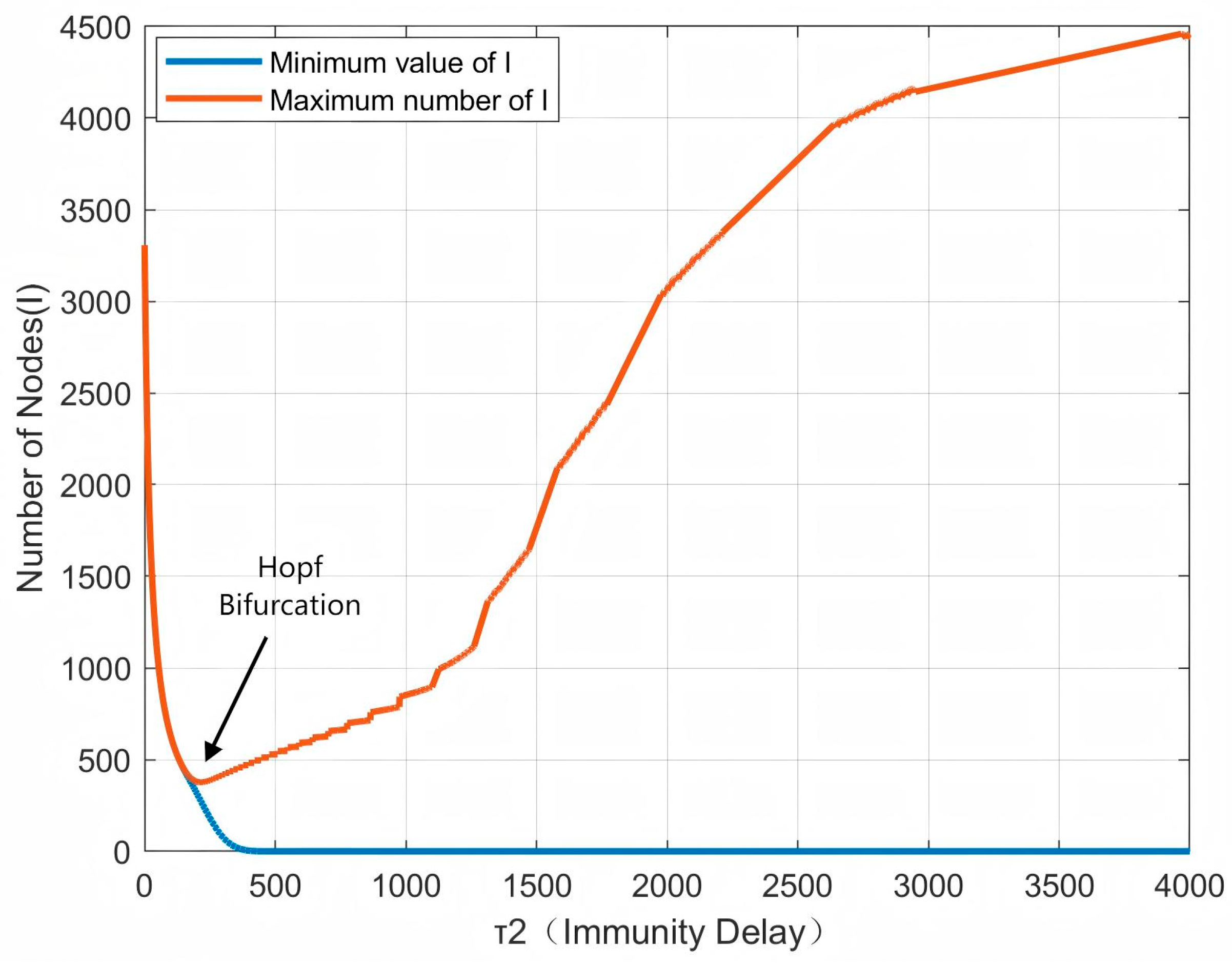
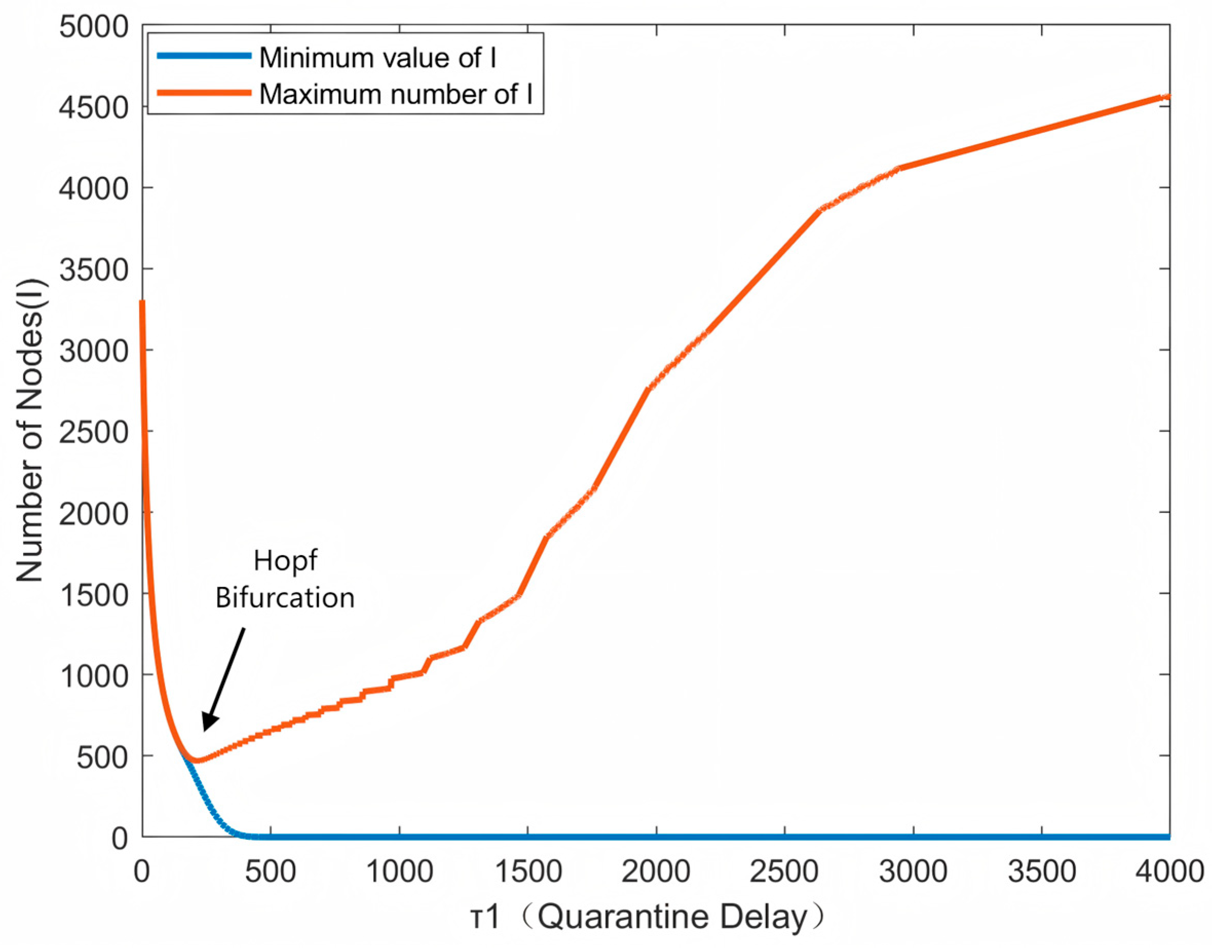
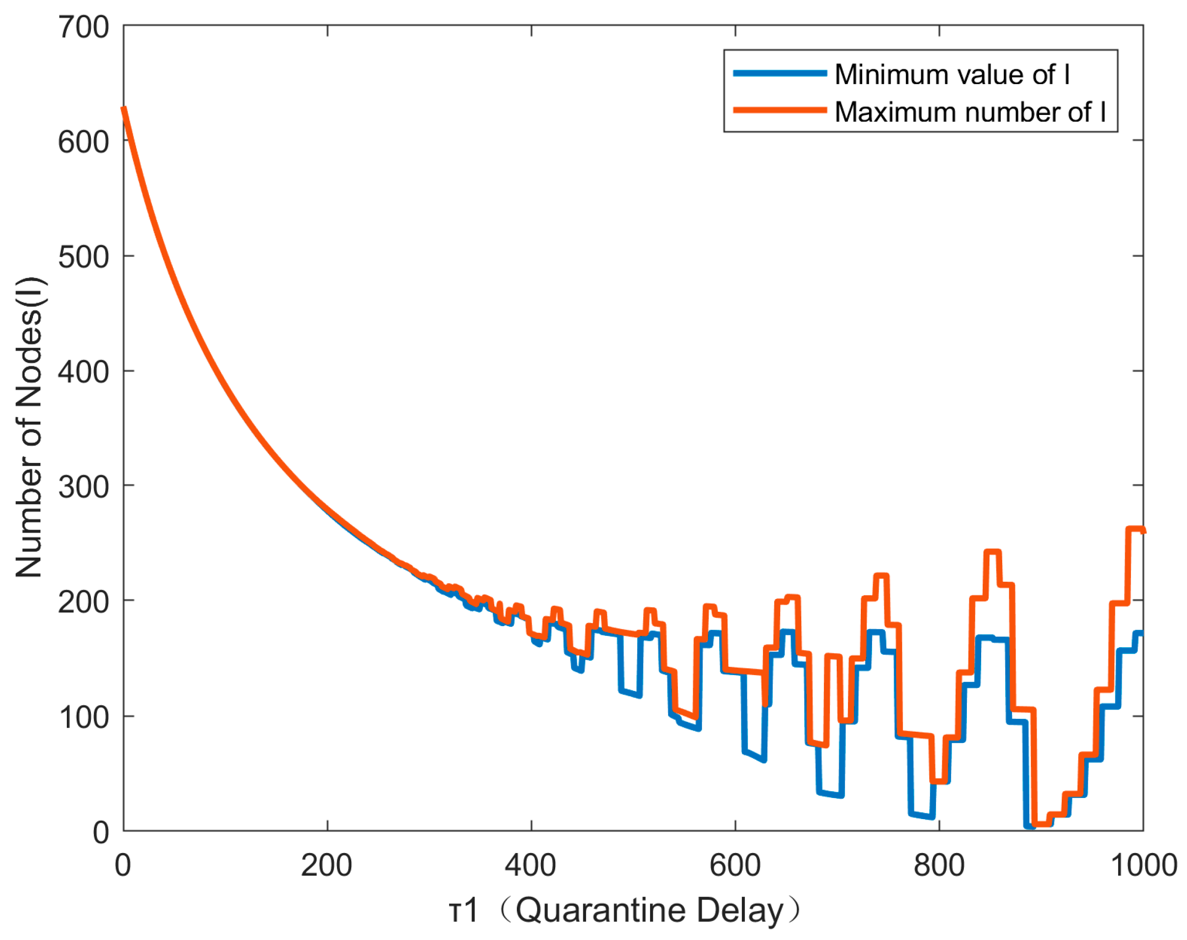
(2) 

When the system satisfies  $d\left(Re\lambda \right)/{d\tau |}_{{\tau }_2={\tau }_2^{*}}$ > 0, the positive equilibrium point  $E^{*}=(S_0^{*},M_0^{*},I_0^{*},{D1}_0^{*},Q_0^{*},R_0^{*},{D2}_0^{*})$  of the system will undergo a Hopf bifurcation at  ${\tau }_2={\tau }_2^{*}$, and the system is destabilized.

(3) 

In the above equation, it can also be seen that the value of  ${\tau }_{1K}^j$ is also affected by  ${\tau }_2$. Hence, the system may have more than one bifurcation point when${\tau }_1,{\tau }_2$  are both greater than 0. This situation needs to be analyzed specifically in the experiment.

4. Numerical Simulation

In the previous section, it has been shown that when ${\mathrm{R}}_0$ < 1, the system is stable without viruses, and when ${\mathrm{R}}_0$ > 1, the system is in a stable or unstable state under different conditions. In this section, numerical experimental analysis was conducted to demonstrate the system’s stability under different conditions and to demonstrate the impact of dual delays on the system.

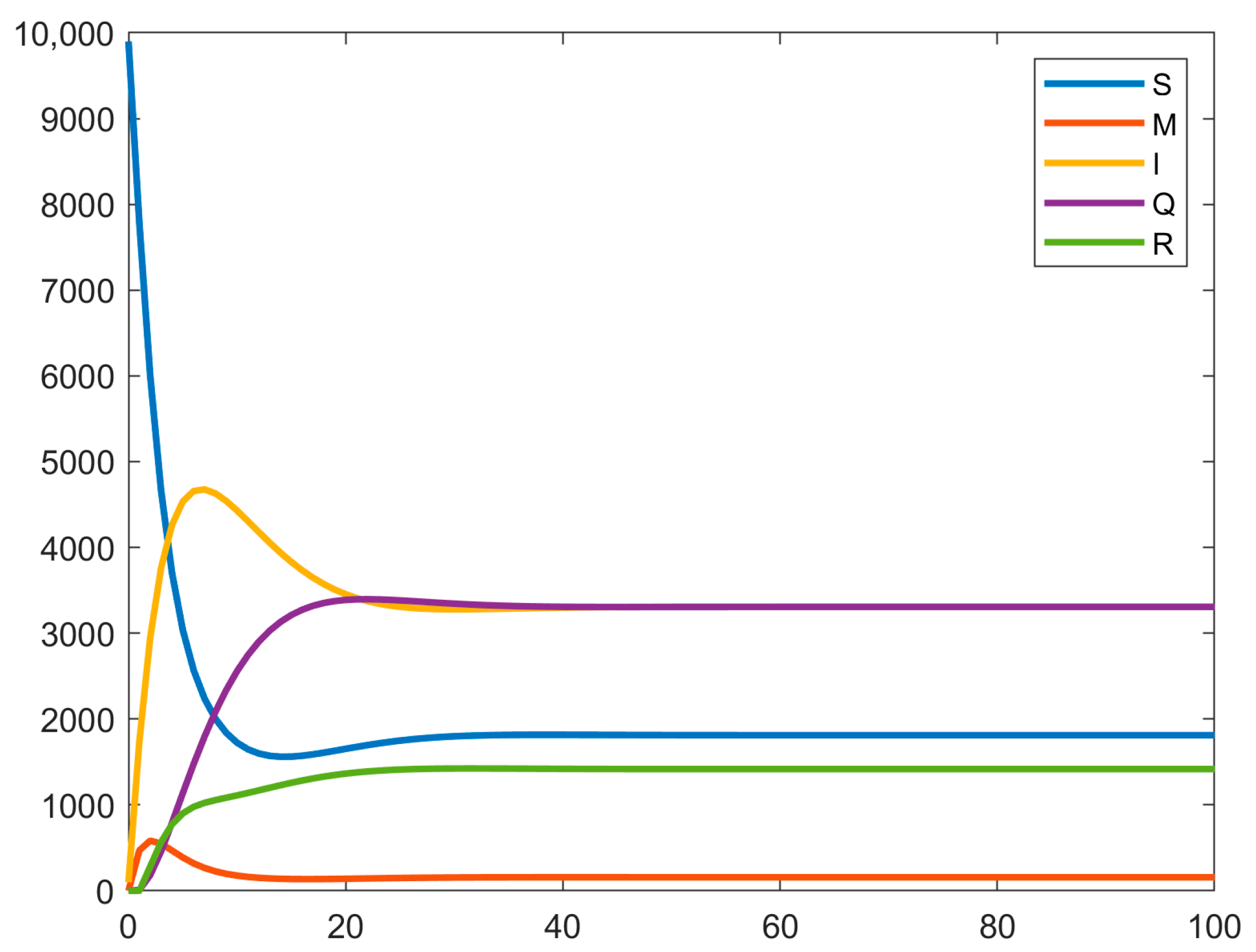
4.1. Equilibrium Analysis

4.1.1. Disease-Free Equilibrium Points

In this section, the stability of the virus-free equilibrium point is verified for different initial values. When ${\mathrm{R}}_0$ < 1, the virus is not capable of spreading in a population enough to sustain a large-scale epidemic. Over time, the number of infected people will gradually decrease, and the virus will eventually disappear. The following figure shows the change in the number of individual nodes in the system when ${\mathrm{R}}_0$ < 1, at different initial values. Figure 2 shows the changes in susceptible nodes, reinforced nodes, infected nodes, isolated nodes, and immune nodes under different initial values, respectively, from which the stability of the virus-free equilibrium point can be proved. Theorem 2, the positive boundedness of the system, can be verified.

4.1.2. Viral Equilibrium Point Stability

When ${\mathrm{R}}_0$ > 1, it is obvious that the system cannot do anything to remove the virus completely; we can only control the virus at an appropriate level. Figure 3 shows how the nodes of the system change when ${\mathrm{R}}_0$ > 1 and when all the nodes reach equilibrium.

4.2. Dual Delayed Impact

After the balanced analysis, in this section, the main focus is to verify the effect of dual delays on malware propagation; in order to analyze it more clearly, the following values of each parameter are taken, and numerical simulations are carried out. In the following simulation, it is assumed that the values of each parameter are as follows: the infection rate $\beta$ assumed = 0.12, the probability of immune node to susceptible node δ = 0.3, the probability of outbreak node to isolation node ε = 0.1, the probability of isolation node to immune node η = 0.1, the probability of infected node to receive the dangerous information to become a reinforced susceptible node λ = 0.8, and the defense capability of susceptible node itself θ = 0.6. In the initial stage, the total number of devices is 10000, and the number of infected devices is assumed to be 100. Due to the existence of dual delays in the system, this section firstly demonstrates the overall nonlinear phenomenon of the model through the bifurcation diagram (in order to better analyze the impact of delay on the system, the nodes entering and exiting the system are set to be fewer).

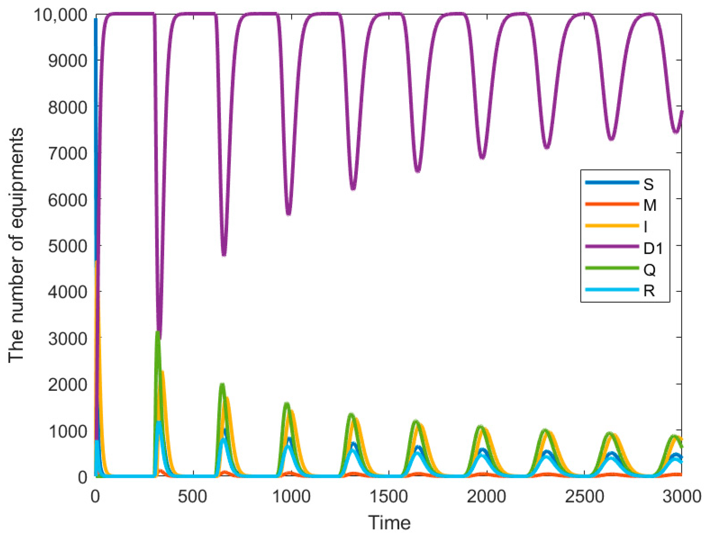
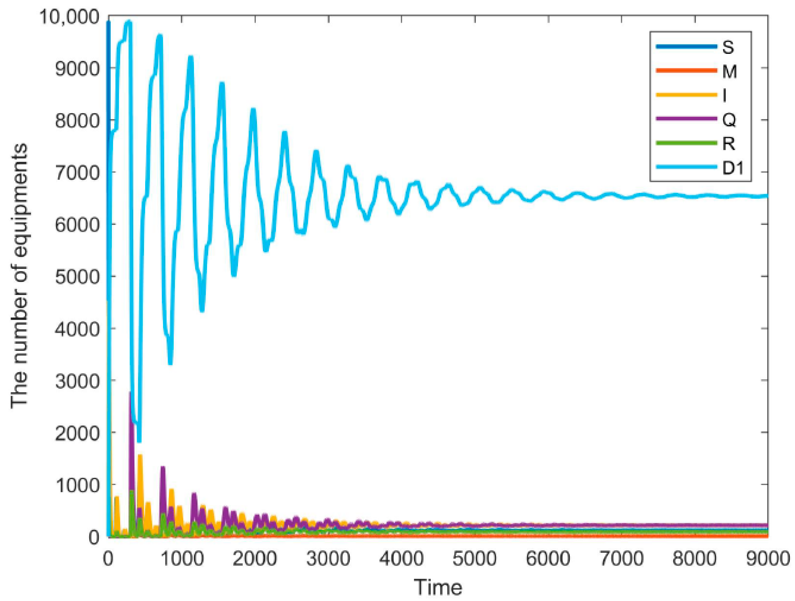
4.2.1. The Case of ${\tau }_1$ = 0

The first discussion is the bifurcation of the system when ${\tau }_1$ = 0, as shown in Figure 4. This case discusses the delay from the immune node to the susceptible node in the system. In the system, some immune nodes, after experiencing the virus and immunity, may experience a virus mutation. The patch is not timely, thus becoming the susceptible node again; whenever the delay value exceeds the threshold value, the system will experience the Hopf bifurcation. Hopf bifurcation may lead to periodic oscillation of the computer system, instability, increased resource consumption, network congestion, and other problems, which can seriously lead to system crash or efficiency degradation. Therefore, considering nonlinear dynamic properties and the Hopf bifurcation phenomenon when designing and optimizing computer systems can help to develop more stable and reliable systems, especially in scenarios that require high availability and stability. That is, in the case of a fork, it is necessary to control the immunization delay of the system to ensure that the malware does not become out of control. In the bifurcation diagram, it can be seen that the threshold ${\tau }_2^{\mathrm{*}}$ of ${\tau }_2$ is 200. The immunization delay needs to be less than a threshold such that the dynamic system eventually reaches equilibrium after oscillations. The curves of the device in different states are shown in Figure 5 (${\tau }_1$ = 0, ${\tau }_2$ = 100) and as shown in Figure 6 (${\tau }_1$ = 0, ${\tau }_2$ = 300), which also corresponds to the single-delay model with only immune delays, and the higher the delays, the higher the final oscillations produced after passing the bifurcation point.

4.2.2. The Case of ${\tau }_2$ = 0

The next phenomenon to be discussed is the bifurcation of the system when ${\tau }_2$ = 0, as shown in Figure 7, which is also equivalent to the single-delay model with only immune delays, and the larger the delays after passing through the bifurcation point, the larger the final oscillations produced; in the bifurcation diagram, it can be seen that the threshold ${\tau }_2^{\mathrm{*}}$ of ${\tau }_2$ is 200. This scenario discusses the isolation delay in the system. In real industrial environments, certain nodes need a certain amount of time to be recognized as infected and to be isolated, which leads to the isolation delay. The isolation delay directly affects the scope and severity of the virus propagation; a longer delay will lead to the rapid spread of the virus in the network, increasing the consumption of the system resources and decreasing the response speed. Isolation delay is common in most industrial scenarios, but longer delays will lead to more serious consequences. The curves of the equipment under different states are shown in Figure 8 (${\tau }_1$ = 100, τ₂ = 0) and Figure 9 (${\tau }_1$ = 300, τ2 = 0). These Figures illustrate the system node diagrams under two conditions where ${\tau }_2$ = 0 and ${\tau }_1$ is respectively less than and greater than ${\tau }_1^{\mathrm{*}}$. It is clearly observable that the system eventually reaches a stable state when ${\tau }_1<{\tau }_1^{\mathrm{*}}$, whereas it becomes unstable when ${\tau }_1>{\tau }_1^{\mathrm{*}}$.

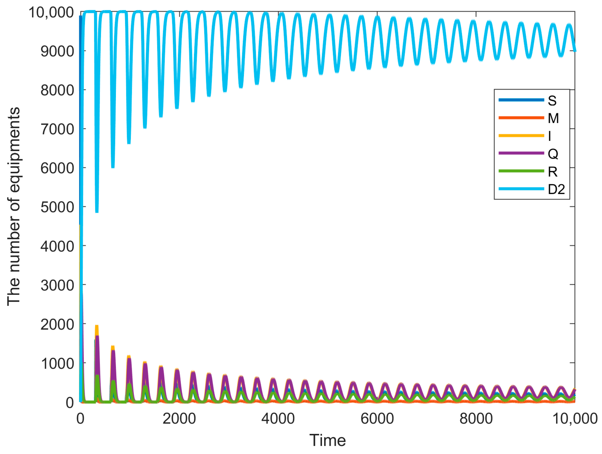
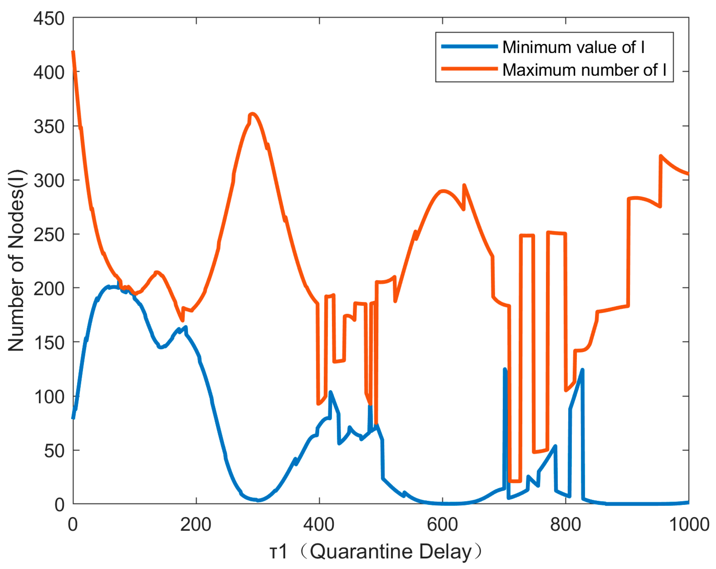
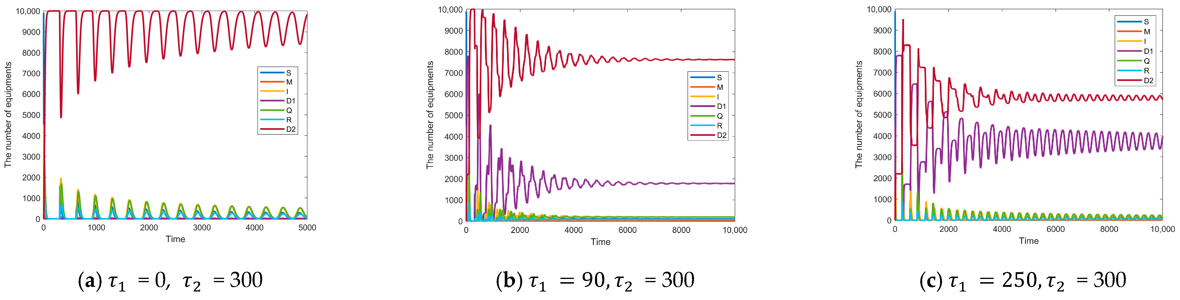
4.2.3. The Case of ${\tau }_1$ > 0, ${\tau }_2<{\tau }_2^{\mathrm{*}}$

We can see in the above experiments that the longer the delay time and the single immune delay after the bifurcation point, the greater the oscillation. Thus, we further discuss the effect of the double delay on the system. Figure 10 below is the bifurcation diagram when ${\tau }_2$= 100. In this bifurcation diagram, it can be clearly found that the system maintains a stable state before ${\tau }_1$= 100 and ${\tau }_2$= 300. However, with the increase in ${\tau }_1$, there are multiple bifurcation points. The following Figure 11 is the node state diagram when ${\tau }_1$= 300 and ${\tau }_2$= 100; the system shown is stable, but in the above experiment, when ${\tau }_1$= 300, ${\tau }_2$= 0, the final state presented is an unstable state. When τ1 increases and ${\tau }_2$ does not change, the system becomes stable, which also shows that these dual delays cannot be discussed separately, and the two are mutually influencing each other.

4.2.4. The Case of ${\tau }_1$ > 0, ${\tau }_2>{\tau }_2^{\mathrm{*}}$

Figure 12 shows the bifurcation diagram of ${\tau }_2>{\tau }_2^{\mathrm{*}}$, it is obvious to find that the bifurcation diagram is very irregular this time, and many abnormal points appear. At the very beginning, ${\tau }_2$ is already in the state of bifurcation. However, at a later time, with the increase in isolation delay, it appears that the node state of the system is gradually stable many times. Figure 13 shows the node state diagrams of the systems with respect to ${\tau }_1$ = 0, ${\tau }_2$ = 300, ${\tau }_1$ = 90, ${\tau }_2$ = 300, ${\tau }_1$ = 250, ${\tau }_2$ = 300. The node state graph of the system and the bifurcation graph are exactly the same as shown in the bifurcation graph. When the isolation time delay increases, the system experiences a transition from instability to stability, which turns to instability again; this situation is more obvious in the phase diagram. Figure 14 also shows the phase diagram of the above cases. The phase diagram is a dynamic system of the relationship between the state variables in the graphical representation. In ${\tau }_1$ = 0, ${\tau }_2$ = 300 and ${\tau }_1$ = 250, ${\tau }_2$ = 300, all the trajectories are far away from a certain point, indicating that these two cases are unstable, while in ${\tau }_1$ = 90, ${\tau }_2$ = 300, all the trajectories converge to a single point, indicating that this case is stable and that the system is globally stable. This suggests that when there is a dual delay in the system, it is not possible to single-handedly control one delay. In this case, we need to specifically analyze the impact of both isolation delay and immunity delay together on the dynamic system. This can be more accurately controlled to ensure the stability of the system and inhibit the propagation of the virus. The aforementioned experiments demonstrate that it is essential to simultaneously regulate the values of both immune delay and isolation delay to maintain the stability of the dynamic system.

In summary, we have found that the dual delays influence each other, which indicates that it is crucial to clarify the impact of different delays on the system’s stability in a dual delay system. For example, as mentioned in Section 4.2.4 above, we cannot simply require the isolation delay to be as small as possible. This is because, when taking into account the immune delay, even a minimal isolation delay may lead to bifurcation. This necessitates a specialized analysis of the effect of the isolation delay on the dynamic system and precise control over it to ensure the system’s stability, thereby suppressing the spread of malicious software.

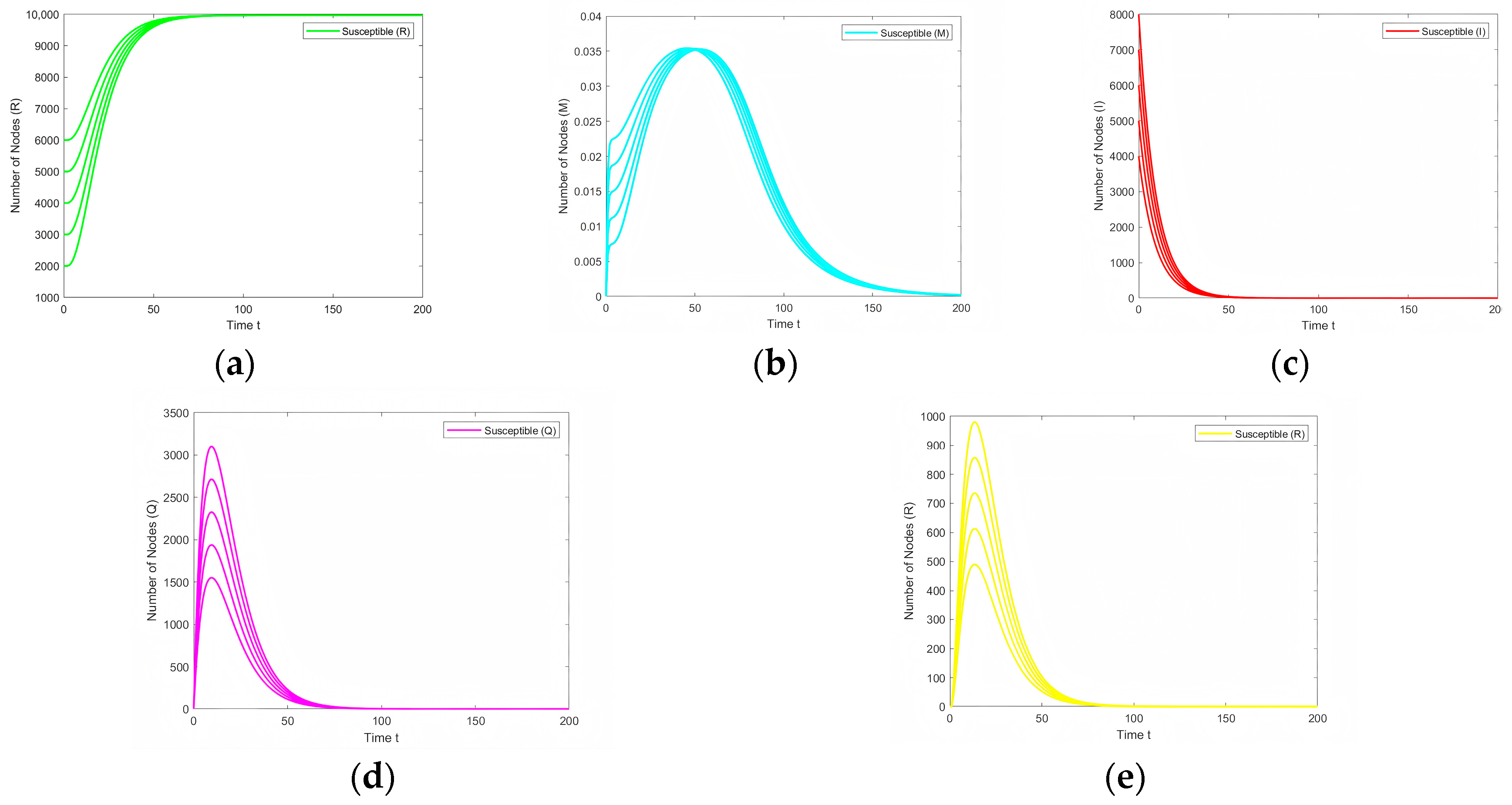
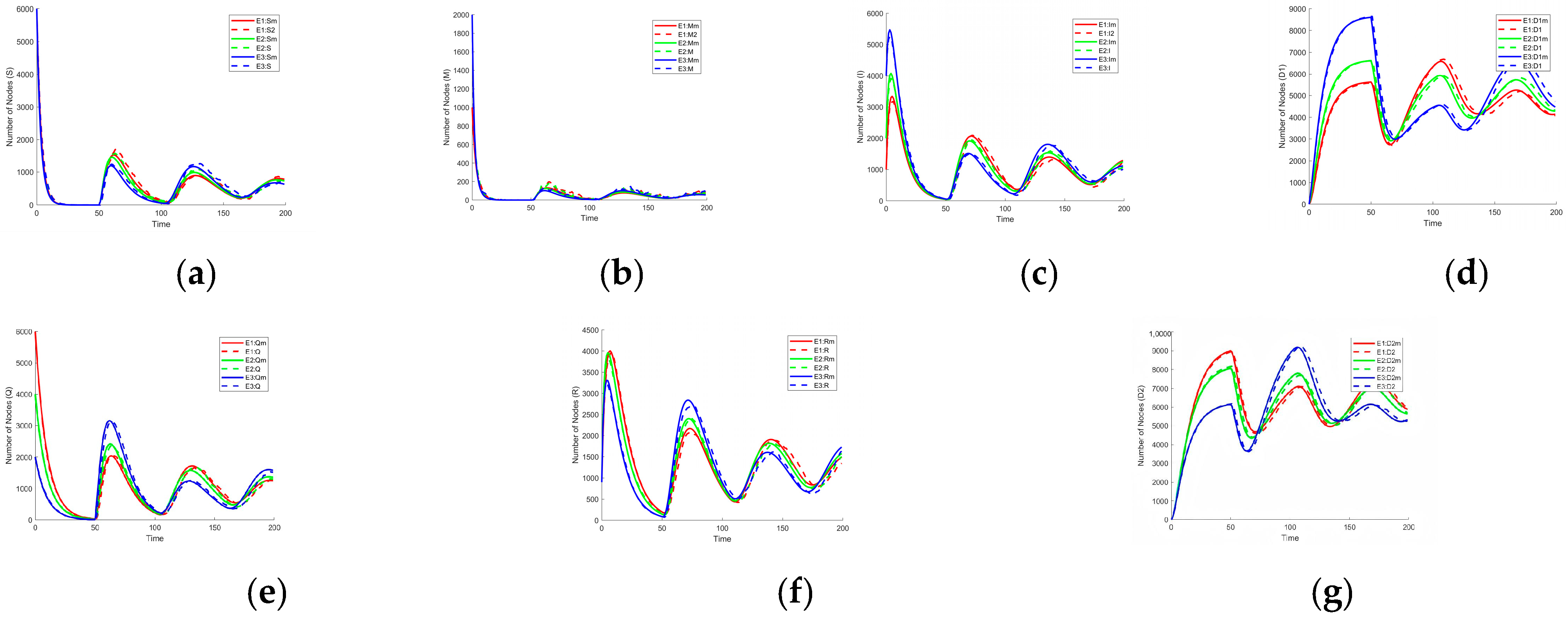
5. Experimental Analysis

This section will conduct a series of experiments based on a real dataset. The dataset originates from a laboratory-scale gas pipeline SCADA system described. It simulates communication and device monitoring scenarios in a gas pipeline SCADA environment.

To present the results with enhanced clarity, we developed a simulation algorithm aligned with the characteristics of our SMIQR model for replicating node transitions observed in real-world data. For effective comparison between empirical observations and differential simulations, distinct labeling conventions are adopted as follows: the baseline results (S, M, I, D1, Q, R, D2) represent real data outputs, while their simulated counterparts (Sm, Mm, Im, D1m, Qm, Rm, D2m) denote differential simulation outcomes.

Under the actual dataset, the SMIDR model evolves with the parameters$\beta$ = 0.12, δ = 0.3, ε = 0.1, η = 0.1, λ = 0.8, θ = 0.6. Below are the sets of initial conditions, respectively, and the evolution of the model under the real dataset is depicted in Figure 15 under the following initials. It can be seen that the differential equations and the actual dataset also have variations. Each state has the same trend with a good fit, indicating the model’s validity. Although some of the results reacting to the actual data differ from the theoretical data, the differences are slight, due to the difference in their simulation methods. However, the final results of both approaches converge to a steady state, showing that the model is very stable under the actual dataset.

• (E1) (S(0), M(0), I(0), D1(0), Q(0), R(0), D2(0)) = (6000,1000,1000,0,6000,900,0).
• (E2) (S(0), M(0), I(0), D1(0), Q(0), R(0), D2(0)) = (6000,2000,2000,0,4000,900,0).
• (E3) (S(0), M(0), I(0), D1(0), Q(0), R(0), D2(0)) = (6000,2000,4000,0,2000,900,0).

In order to control the spread of industrial viruses, it is essential to understand some of the parameters in the system that affect the spread of viruses, which play a significant role in controlling the spread of viruses in the system faster and reducing the number of viruses in the system. There is a special parameter among all the parameters: the infection inhibition factor in the non-dominant infection rate. This parameter represents a saturation characteristic of the infection rate in the model. When the infection inhibition factor a is more prominent, the overall infection rate is smaller, the spread is slower, and fewer infected people are in the system when reaching the equilibrium, and when the infection inhibition factor a is smaller, the overall infection rate is more significant, the spread is faster, and the more infected people are in the system when reaching the equilibrium. The more-infected people are in the system at equilibrium. As shown in Figure 16, which is the node diagram for the system corresponding to four groups of a = 0.5, a = 1, a = 1.5, and a = 2 with other parameters being the same, it can be clearly seen that as the infection inhibition factor gradually increases, the infected nodes reach their maximum value more quickly. There are fewer infected nodes in the steady-state system.

The infection suppression factor describes the effect that the infection rate gradually slows down with the increase in the number of infected nodes, and this infection suppression factor can also be reflected in the SCADA industrial network, which is mainly reflected in the topology of the network, the traffic characteristics, the characteristics of the node equipment, security measures, the virus propagation mechanism, and the external environmental factors, etc. For example, in an industrial network, which belongs to a highly centralized network, the network traffic is enormous, which will have an impact on the infection suppression factor. For a highly connected network, the more connections between the nodes, the faster the virus spreads, and the infection rate may be more likely to reach saturation. In this kind of network environment, we should prioritize the isolation of devices with high-density and more connected nodes when we take isolation to slow down the propagation rate. The saturation effect of the infection rate, a value, is based on the combined results of a variety of factors. Through a comprehensive analysis of the above factors, you can determine the value of the saturation effect for a particular industrial network environment to enable the corresponding countermeasures to reduce the infection inhibition factor, such that the system reaches equilibrium when it has fewer diseased nodes and performs better.

Similarly, the parameter θ, which represents the magnitude of defense capability in the enhanced state (M), offers crucial insights into how nodes can autonomously strengthen their defenses. When a susceptible RTU node receives danger signals from infected counterparts and transitions to the enhanced state (M), a high θ value indicates that these internal defense mechanisms are highly efficient. Nodes with a strong θ are more likely to directly transition to the immune state (R) upon encountering a virus, effectively preventing infection. Conversely, a lower θ implies that the node’s self-defense capabilities are relatively weak. In such cases, despite entering the enhanced state, the node may still succumb to infection and transition to the infected state (I). As shown in Figure 17, the number of I nodes in the system corresponding to the four cases of θ = 0.5, θ = 0.6, θ = 0.7, θ = 0.9 respectively with other parameters being the same, it can be clearly seen that the peak of the infected nodes and the number of the stabilized system decrease with the increase in θ, which indicates that the enhancement in θ can have a certain inhibitory effect on the propagation of the virus in the system.

In the industrial network scenario, θ can be seen as a measure of the effectiveness of the built-in security mechanisms within RTU nodes. For example, modern RTUs may be equipped with advanced firmware that contains heuristic algorithms capable of detecting and neutralizing emerging threats. A lower θ may resemble a situation where the RTU’s security features are outdated or insufficient, leaving the RTU vulnerable to attack even after receiving alerts of potential threats. By analyzing the impact of θ on the overall system, we can better understand how to optimize the design and configuration of RTU nodes, ensuring they are better equipped to withstand cyberattacks in the complex landscape of SCADA industrial networks.

Together, the infection suppression factor a and the self-defense capability parameter θ provide a comprehensive framework for enhancing the security resilience of SCADA systems against malware propagation.

6. Model Comparison

In this section, to quantitatively validate the advantages of the proposed SMLBR model, we conducted comparative experiments with two representative models: the SLBR model [31] and the SEIQP model [15].

This four-state model (S: Susceptible, L: Latent, B: Burst, R: Recovered) is compared with our SMIQR model. Our model introduces two additional states: M (Enhanced Susceptibility through risk information exchange) and Q (Quarantined). This comparison aims to verify whether the control strategies (risk information propagation and quarantine) in SMIQR effectively improve virus containment. The dynamic equations of SLBR are as follows:

$$\left\{\begin{array}{l}{\displaystyle \frac{dS}{dt}}=b-\beta S(L+B)-\mu S\hfill \\ {\displaystyle \frac{dL}{dt}}=(1-p)\beta (L+B)S-\gamma L+\epsilon B-\mu L\hfill \\ {\displaystyle \frac{dB}{dt}}=p\beta (L+B)S+\gamma L-\epsilon B-\alpha B-\mu B\hfill \\ {\displaystyle \frac{dR}{dt}}=\alpha B-\mu R.\hfill \end{array}\right.,$$

(42)

And the second model SEIQR model has five states which are S (Susceptible state), E (Exposed state), I (Infected state), I (Infected state), Q (Quarantine state), R (Immune state). In this model, the authors also proposed controlling the spread of viruses through isolation and patching using the same isolation approach as proposed in this model. The main difference between the SMIQR model and the SEIQR model is that the prevention and control strategies used are different. The approach taken in this paper is through information dissemination. Hence, the significance of comparing it with this model focuses more on whether or not this approach helps to reduce the number of infected nodes. Its dynamic equations are as follows:

$$\left\{\begin{array}{l}{\displaystyle \frac{dS}{dt}}=(\eta +\xi )P+\theta I-\sigma S-\beta SI-\rho S\hfill \\ {\displaystyle \frac{dE}{dt}}=\sigma S+\beta SI-\gamma E\hfill \\ {\displaystyle \frac{dI}{dt}}=\gamma E-\theta I-\delta I\hfill \\ {\displaystyle \frac{dQ}{dQ}}=\delta I-\epsilon Q\hfill \\ {\displaystyle \frac{dP}{dt}}=\rho S+\epsilon Q-(\eta +\xi )P.\hfill \end{array},\right.$$

(43)

The initial node values for the three models are as follows:

SLBR: (S(0), L(0), B(0), R(0)) = (3000, 3000, 3000, 1000)

SEIQP: (S(0), E(0), I(0), Q(0), P(0)) = (3000, 3000, 3000, 0, 1000)

SMIQR: (S(0), M(0), I(0), Q(0), R(0)) = (3000, 1000, 3000, 2000, 1000)

The specific parameters for each model are shown in

Table 1. The specific parameters for the three models.

	Parameter	${\mathbf{R}}_0$	$\mathit{\beta }$	a	b	$\mathit{\epsilon }$	$\mathit{\mu }$	$\mathit{\alpha }$	$\mathit{\delta }$	$\mathit{\eta }$	$\mathit{\lambda }$	$\mathit{\theta }$	$\mathit{\gamma }$	$\mathit{\zeta }$	p	$\mathit{\sigma }$
Model
SLBR		1.52	0.35	—	0.2	0.4	0.2	0.18	—	—	—	—	0.1	—	—
SEIQP		1.58	0.6	—	—	0.3	—	—	0.15	0.3	—	0.2	0.3	0.2	0.04	0.15
SMIQR		1.51	0.35	1	0.2	0.1	0.2		0.3	0.1	0.9	0.7	—	—	—	—

. However, because the meaning of the parameters used for the three models are different, it is impossible to completely realize the unity of the parameter values, in order to control the infectiousness of the virus in the three models, in this experiment, the reusable number R₀ is used as a standard, to control the same value of R₀, the same R₀ indicates the reproduction ability of the virus, and the difference in the number of nodes in the results is due to the strategy not used in the model itself. The specific parameters shown in the graphs indicate that R₀ is basically the same under the three models, and the experiment has some reference value.

First we observe the evolution of S nodes and R nodes under the three models, as shown in the Figure 18, the number of S and R nodes of the three models eventually stabilizes, after stabilization it shows that our model has the highest number of S, R, the SLBR model has a higher number of S, and the number of R nodes is less, indicating that more node states are in the S state after this model reaches the steady state, and the SLBR model has the lowest number of S, and the higher number of R that indicates that more node states are in S state after reaching steady state in SEIQR model. The experimental results show that the SMIQR model has more S and R nodes, which also indicates that the immunity of the nodes is improved after taking the preventive and control measures in this model.

In both network systems and SCADA-based industrial systems, latent nodes and infected nodes are the most critical state variables due to their inherent infectiousness and potential to cause widespread damage. Theoretically, minimizing their numbers can significantly reduce system-wide losses. In our study, we combine the latent and burst states into a unified metric $\tilde{\mathrm{I}}$, which represents the total number of individuals in the infection cycle during viral propagation. Figure 19 below illustrates $\tilde{\mathrm{I}}$ evolution across the three models:

As shown in Figure 19, the SMIQR model achieves the lowest $\tilde{\mathrm{I}}$ compared to the baseline models. This demonstrates its superior performance in viral containment; it effectively suppresses viral spread during epidemic phases, maintains infected nodes at minimal levels, and thereby enhances overall system security. These results underscore that SMIQR’s integrated strategies (e.g., risk-aware immunization and dynamic quarantine) are highly effective in mitigating infection cycles and reducing systemic risks.

7. Conclusions

(1)

This paper analyzes the structure of SCADA systems and the security threats they face and proposes a novel SCADA industrial network virus propagation model, SMIQR. The construction of this model is based on the phenomenon observed in social networks, financial markets, and urban transportation systems, where “immune” nodes reduce virus propagation through information exchange. It simulates the process by which infected nodes transmit dangerous information to uninfected nodes. The model considers the impact of information transmission between nodes and allows nodes to enhance their defensive capabilities after receiving dangerous information, thereby improving the overall antivirus capability of the group of nodes.

(2)

Methodologically, this paper adopts the assumptions of nonlinear infection rates and dual delay, which align more closely with the actual conditions of industrial control networks. Unlike the commonly used bilinear infection rate assumption in existing research, this paper considers the uncertainty in the behavior of susceptible devices, thereby introducing the concept of nonlinear infection rates and incorporating isolation strategies to effectively control virus propagation.

(3)

Based on the characteristics of industrial viruses and the model, this paper designs an algorithm using a real dataset and validates the model’s effectiveness through this dataset.

(4)

Building on this foundation, the paper investigates the propagation of malware in industrial control networks, the stability of dynamic systems, and the Hopf bifurcation phenomenon. The study finds that in a dual delay system, the dual delays interact and cannot be simply separated into two single-delay systems for individual discussion. During the research process, it is essential to clarify the impact of different delays on system stability, and one cannot merely require one delay to be as small as possible. This is because, in a dual delay system, a small value of the other delay may still lead to bifurcation even if one delay is fixed. Therefore, it is necessary to specifically analyze the combined impact of the dual delays on the dynamic system and precisely control them to ensure system stability, thereby suppressing the spread of malware.

(5)

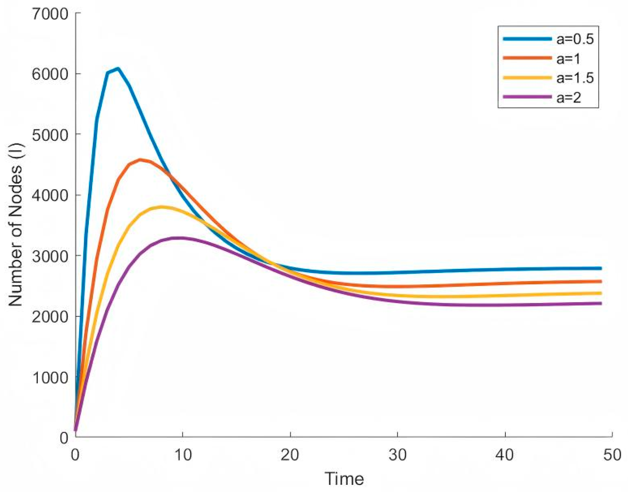
Furthermore, through the analysis of the infection suppression factor, it is found that when implementing isolation measures, priority should be given to isolating devices with high connection density and more connected nodes to slow down the virus propagation rate. The value of the infection suppression factor *a* is a comprehensive result of multiple factors. By comprehensively analyzing the characteristics of the SCADA system, the saturation effect value suitable for this industrial network can be determined, enabling the formulation of corresponding strategies to reduce the infection suppression factor and achieve a system equilibrium with fewer infected nodes.

However, our current model is constrained by its closed single-network system assumption, which cannot characterize cross-network propagation paths. Additionally, the oversimplified premise of uniform security policies across networks fails to reflect real-world complexity. To address these limitations, our ongoing research extends the baseline homogeneous model through the following enhancements:

• Degree-dependent parameters to quantify propagation capability differences between hub nodes and edge nodes.
• Enhanced cross-layer propagation terms characterizing viral penetration through gateway devices.
• Dynamic threshold adaptation based on real-time topological features.

Additionally, further research is needed to explore how the dual delays specifically interact to affect system stability and how to determine the specific ranges of the dual delays while ensuring system stability. These issues require further refinement in subsequent studies.

References

- Gaushell, D.J.; Darlington, H.T. Supervisory control and data acquisition. Proc. IEEE 1987, 75, 1645–1658. [Google Scholar] [CrossRef]
- Gelmini, A. 5G Scada Based Control System. Ph.D. Thesis, University of South Wales, Cardiff, UK, 2024. [Google Scholar]
- Wang, J.; Si, C.; Wang, Z.; Fu, Q. A New Industrial Intrusion Detection Method Based on CNN-BiLSTM. Comput. Mater. Contin. 2024, 79, 4297. [Google Scholar] [CrossRef]
- Hudedmani, M.G.; Umayal, R.M.; Kabberalli, S.K.; Hittalamani, R. Programmable logic controller (PLC) in automation. Adv. J. Grad. Res. 2017, 2, 37–45. [Google Scholar] [CrossRef]
- Zhang, H.; Tan, J.; Liu, X.; Huang, S.; Hu, H.; Zhang, Y. Cybersecurity threat assessment integrating qualitative differential and evolutionary games. IEEE Trans. Netw. Serv. Manag. 2022, 19, 3425–3437. [Google Scholar] [CrossRef]
- Kephart, J.O.; White, S.R. Directed-graph epidemiological models of computer viruses. In Computation: The Micro and the Macro View; World Scientific: Singapore, 1992; pp. 71–102. [Google Scholar]
- Kephart, J.O.; White, S.R.; Chess, D.M. Computers and epidemiology. IEEE Spectr. 1993, 30, 20–26. [Google Scholar] [CrossRef]
- Kephart, J.O.; White, S.R. Measuring and modeling computer virus prevalence. In Proceedings of the 1993 IEEE Computer Society Symposium on Research in Security and Privacy, Oakland, CA, USA, 24–26 May 1993; IEEE: Piscataway, NJ, USA, 1993; pp. 2–15. [Google Scholar]
- Wo, K. A contribution to the mathematical theory of epidemics. Proc. R. Soc. A 1927, 115, 700–721. [Google Scholar]
- Serazzi, G.; Zanero, S. Computer virus propagation models. In International Workshop on Modeling, Analysis, and Simulation of Computer and Telecommunication Systems; Springer: Berlin/Heidelberg, Germany, 2003; pp. 26–50. [Google Scholar]
- Wu, J.; Zhang, X.; Zhu, X.; Xu, X. A variant sirs virus spreading model. In Proceedings of the 2017 International Conference on Computer Systems, Electronics and Control (ICCSEC), Dalian, China, 25–27 December 2017; IEEE: Piscataway, NJ, USA, 2017; pp. 121–124. [Google Scholar]
- Dodds, P.S.; Watts, D.J. A generalized model of social and biological contagion. J. Theor. Biol. 2005, 232, 587–604. [Google Scholar] [CrossRef]
- Zhao, T.; Zhang, Z.; Upadhyay, R.K. Delay-induced Hopf bifurcation of an SVEIR computer virus model with nonlinear incidence rate. Adv. Differ. Equ. 2018, 2018, 256. [Google Scholar] [CrossRef]
- Safar, J.L.; Tummala, M.; McEachen, J.C.; Bollmann, C. Modeling worm propagation and insider threat in air-gapped network using modified SEIQV model. In Proceedings of the 2019 13th International Conference on Signal Processing and Communication Systems (ICSPCS), Gold Coast, QLD, Australia, 16–18 December 2019; pp. 1–6. [Google Scholar]
- Sulaiman, M.; Khan, A.; Ali, A.N.; Laouini, G.; Alshammari, F.S. Quantitative analysis of worm transmission and insider risks in air-gapped networking using a novel machine learning approach. IEEE Access 2023, 11, 111034–111052. [Google Scholar] [CrossRef]
- Tang, W.; Liu, Y.J.; Chen, Y.L.; Yang, Y.X.; Niu, X.X. SLBRS: Network virus propagation model based on safety entropy. Appl. Soft Comput. 2020, 97, 106784. [Google Scholar] [CrossRef]
- Zhang, X.; Gan, C. Global attractivity and optimal dynamic countermeasure of a virus propagation model in complex networks. Phys. A Stat. Mech. Its Appl. 2018, 490, 1004–1018. [Google Scholar] [CrossRef]
- Jun, W.; Haoyang, G. Virtual force field coverage algorithms for wireless sensor networks in water environments. Int. J. Sens. Netw. 2020, 32, 174–181. [Google Scholar] [CrossRef]
- Shen, S.; Li, H.; Han, R.; Vasilakos, A.V.; Wang, Y.; Cao, Q. Differential game-based strategies for preventing malware propagation in wireless sensor networks. IEEE Trans. Inf. Forensics Secur. 2014, 9, 1962–1973. [Google Scholar] [CrossRef]
- Matta, V.; Di Mauro, M.; Longo, M.; Farina, A. Cyber-threat mitigation exploiting the birth–death–immigration model. IEEE Trans. Inf. Forensics Secur. 2018, 13, 3137–3152. [Google Scholar] [CrossRef]
- Carcano, A.; Coletta, A.; Guglielmi, M.; Masera, M.; Fovino, I.N.; Trombetta, A. A multidimensional critical state analysis for detecting intrusions in SCADA systems. IEEE Trans. Ind. Inform. 2011, 7, 179–186. [Google Scholar] [CrossRef]
- Sheng, C.; Yao, Y.; Fu, Q.; Yang, W.; Liu, Y. Study on the intelligent honeynet model for containing the spread of industrial viruses. Comput. Secur. 2021, 111, 102460. [Google Scholar] [CrossRef]
- Wang, Y.; Gu, D.; Peng, D.; Chen, S.; Yang, H. Stuxnet vulnerabilities analysis of scada systems. In Proceedings of the International Conference on Network Computing and Information Security, Shanghai, China, 7–9 December 2012; Springer: Berlin/Heidelberg, Germany, 2012; pp. 640–646. [Google Scholar]
- Valentine, S.E. PLC Code Vulnerabilities Through SCADA Systems; University of South Carolina: Columbia, SC, USA, 2013. [Google Scholar]
- Stanković, A.M.; Tomsovic, K.L.; De Caro, F.; Braun, M.; Chow, J.H.; Čukalevski, N.; Dobson, I.; Eto, J.; Fink, B.; Hachmann, C.; et al. Methods for analysis and quantification of power system resilience. IEEE Trans. Power Syst. 2022, 38, 4774–4787. [Google Scholar] [CrossRef]
- He, J.; Li, Y.; Tang, J.; Wang, H.; Yang, G.; Li, T.; Lan, X. An Immune Knowledge-Driven SCADA-Based Industrial Virus Propagation Model. IEEE Internet Things J. 2024, 11, 29956–29970. [Google Scholar] [CrossRef]
- Zhang, R.; Cao, Z.; Yang, S.; Si, L.; Sun, H.; Xu, L.; Sun, F. Cognition-driven structural prior for instance-dependent label transition matrix estimation. IEEE Trans. Neural Netw. Learn. Syst. 2024, 36, 3730–3743. [Google Scholar] [CrossRef]
- Zhang, R.; Tan, J.; Cao, Z.; Xu, L.; Liu, Y.; Si, L.; Sun, F. Part-aware correlation networks for few-shot learning. IEEE Trans. Multimed. 2024, 26, 9527–9538. [Google Scholar] [CrossRef]
- Wu, Y.; Ru, Y.; Lin, Z.; Liu, C.; Xue, T.; Zhao, X.; Chen, J. Research on cyber attacks and defensive measures of power communication network. IEEE Internet Things J. 2022, 10, 7613–7635. [Google Scholar] [CrossRef]
- Nankya, M.; Chataut, R.; Akl, R. Securing industrial control systems: Components, cyber threats, and machine learning-driven defense strategies. Sensors 2023, 23, 8840. [Google Scholar] [CrossRef]
- Zhu, Q.; Zhang, G.; Luo, X.; Gan, C. An industrial virus propagation model based on SCADA system. Inf. Sci. 2023, 630, 546–566. [Google Scholar] [CrossRef]
- Wang, J.; Wang, N.; Wang, H.; Cao, K.; El-Sherbeeny, A.M. GCP: A multi-strategy improved wireless sensor network model for environmental monitoring. Comput. Netw. 2024, 254, 110807. [Google Scholar] [CrossRef]
- Wang, J.; Luo, D.; Peng, F.; Chen, W.; Liu, J.; Zhang, H. Wireless sensor deployment optimisation based on cost, coverage, connectivity, and load balancing. Int. J. Sens. Netw. 2023, 41, 126–135. [Google Scholar] [CrossRef]
- Irmak, E.; Erkek, İ. An overview of cyber-attack vectors on SCADA systems. In Proceedings of the 2018 6th International Symposium on Digital Forensic and Security (ISDFS), Antalya, Turkey, 22–25 March 2018; IEEE: Piscataway, NJ, USA, 2018; pp. 1–5. [Google Scholar]
- Knapp, E.D. Industrial Network Security: Securing Critical Infrastructure Networks for Smart Grid, SCADA, and Other Industrial Control Systems; Elsevier: Amsterdam, The Netherlands, 2024. [Google Scholar]
- Fu, Q.; Wang, J.; Si, C.; Liu, J. The Effect of Key Nodes on the Malware Dynamics in the Industrial Control Network. Comput. Mater. Contin. 2024, 79, 329. [Google Scholar] [CrossRef]
- Veblen, T.T. Regeneration dynamics. Plant Succession Theory Predict. 1992, 11, 152–187. [Google Scholar]
- Diekmann, O.; Heesterbeek, J.A.P.; Roberts, M.G. The construction of next-generation matrices for compartmental epidemic models. J. R. Soc. Interface 2010, 7, 873–885. [Google Scholar] [CrossRef]
- Yuan, H.; Chen, G. Network virus-epidemic model with the point-to-group information propagation. Appl. Math. Comput. 2008, 206, 357–367. [Google Scholar] [CrossRef]
- Yang, J.; Zhang, F.; Wang, X. A class of SIR epidemic model with saturation incidence and age of infection. In Proceedings of the Eighth ACIS International Conference on Software Engineering, Artificial Intelligence, Networking, and Parallel/Distributed Computing (SNPD 2007), Qingdao, China, 30 July 2007; IEEE: Piscataway, NJ, USA, 2007; Volume 1, pp. 146–149. [Google Scholar]