Abstract
The Chinese stock market, one of the largest and most dynamic emerging markets, is characterized by individual investor dominance and strong policy influence, resulting in high volatility and complex dynamics. These distinctive features pose substantial challenges for accurate forecasting. Existing models like RNNs, LSTMs, and Transformers often struggle with non-stationary data and long-term dependencies, limiting their forecasting effectiveness. This study proposes a hybrid forecasting framework integrating the Non-stationary Autoformer (NSAutoformer), LASSO feature selection, and financial sentiment analysis. LASSO selects key features from diverse structured variables, mitigating multicollinearity and enhancing interpretability. Sentiment indices are extracted from investor comments and news articles using an expanded Chinese financial sentiment dictionary, capturing psychological drivers of market behavior. Experimental evaluations on the Shanghai Stock Exchange Composite Index show that LASSO-NSAutoformer outperforms the NSAutoformer, reducing MAE by 8.75%. Additional multi-step forecasting and time-window analyses confirm the method’s effectiveness and stability. By integrating multi-source data, feature selection, and sentiment analysis, this framework offers a reliable forecasting approach for investors and researchers in complex financial environments.
1. Introduction
The Chinese stock market has grown rapidly, attracting investors seeking to anticipate trends for financial gain. However, stock price volatility complicates forecasting and amplifies investment risks. Accurate predictions are essential for both individuals and organizations, guiding investment decisions and risk management. For investors, forecasts support decisions on buying, selling, or applying stop-loss strategies. For organizations, reliable forecasts support trading, asset allocation, and portfolio management [1]. Yet, stock price movements are inherently complex and nonlinear [2].
As financial time series data, stock prices are highly volatile and subject to random noise, making prediction particularly challenging [3]. Over the years, researchers have explored various forecasting approaches. Traditional statistical models, such as Moving Average (MA) [4], Auto-Regressive Moving Average (ARMA) [5], and Auto-Regressive Integrated Moving Average (ARIMA) [6], as well as volatility models like Auto-Regressive Conditional Heteroskedasticity (ARCH) [7] and Generalized Auto-Regressive Conditional Heteroskedasticity (GARCH) [8], have been widely applied. Among them, ARIMA performs well on time series with clear trends and seasonality. However, ARIMA assumes smooth data, limiting its ability to model highly volatile stock prices [9]. These models depend on predefined variable selection and linear assumptions, making it difficult to capture complex, nonlinear patterns in large-scale, high-dimensional financial data. Traditional econometric methods cannot effectively handle unstructured alternative data, leading to a growing shift toward machine learning approaches.
Machine learning methods such as K-Nearest Neighbor (KNN) [10], Support Vector Machine (SVM) [11], and random forests [12] have shown promise in modeling nonlinear relationships and complex market dynamics. Nevertheless, these approaches often encounter challenges such as feature selection and overfitting. To further improve forecasting performance and autonomously extract intricate patterns from financial time series, researchers have turned to deep learning techniques. Models such as Artificial Neural Networks (ANNs), Convolutional Neural Networks (CNNs) [13], Recurrent Neural Networks (RNNs) [14], Long Short-Term Memory (LSTM) networks [15], and Gated Recurrent Units (GRUs) [16] have been widely explored. While RNNs capture temporal dependencies, they suffer from gradient instability. LSTM and GRU alleviate this issue but still face challenges such as overfitting and high training complexity.
Since Vaswani et al. introduced the Transformer in 2017 [17,18], Transformer-based models have been widely used in time series forecasting with notable success. Based on attention mechanisms, the Transformer effectively captures long-term dependencies in sequential data, addressing the limitations of traditional RNN-based models. In 2021, Zhou et al. proposed the Informer model, which optimized the attention mechanism, mitigating long-term information loss [19]. Following these advancements, researchers have further refined Transformer-based architectures and applied them to stock price prediction [20].
The non-stationary and highly volatile nature of financial markets poses considerable challenges for accurate forecasting. Traditional models often fail to capture the complex, nonlinear structures embedded in stock price movements. To address this, we propose the Non-stationary Autoformer (NSAutoformer), which extends the Non-stationary Transformers framework to the Autoformer [21,22], enhancing adaptability to evolving financial data. The model enhances adaptability by decomposing time series into trend and seasonal components and adjusting to distributional shifts. To further improve forecasting, we incorporate the LASSO algorithm and sentiment analysis, forming a multi-source data approach. The LASSO-NSAutoformer is empirically validated on the Chinese stock market index, showing stable, reliable, and superior predictive performance.
The Chinese stock market is one of the largest and most dynamic emerging markets, with a high proportion of individual investors, making it highly sensitive to sentiment. Compared to developed markets, Chinese individual investors are generally less experienced and prone to herd behavior, often reacting to media reports and peer suggestions with panic buying or selling. Moreover, government policies exert strong influence on the market. The active online environment, including financial social media and investor forums, provides a wealth of sentiment-rich data, supporting broad coverage for this study. These characteristics offer a unique opportunity to evaluate our proposed approach in a complex, sentiment-sensitive market.
The proposed framework comprises three main stages. First, the LASSO algorithm selects relevant features from 49 structured variables, including historical prices, trading data, technical indicators, composite indices, and other market information. Second, a Chinese financial sentiment dictionary is used to analyze investor comments and news, producing two sentiment indices incorporated into the forecasting model. Finally, hyperparameters are tuned using Optuna to improve model performance. Comparative experiments show that the proposed method outperforms traditional models, including RNN, GRU, LSTM, and Transformer-based architectures. Notably, LASSO-based feature selection enhances accuracy by identifying key predictors, reducing overfitting and computational complexity. Additionally, the sentiment indices capture investor psychology, which correlates with market fluctuations. By analyzing key factor interactions, this study provides deeper insight into market dynamics. Combining fundamental and sentiment-driven variables allows the model to more accurately reflect real-world market behavior and improve forecasting performance.
The main work accomplished in the article is as follows:
- 1.
- This study incorporates multiple factors, including trading data, technical indicators, geopolitical events, epidemics, public sentiment, and cross-market influences, with a focus on sentiment analysis. A Chinese financial sentiment dictionary is constructed to extract sentiment from investor comments and news articles.
- 2.
- We propose NSAutoformer by extending the Non-stationary Transformers framework to the Autoformer architecture. This architecture retains the series decomposition mechanism and improves the ability to model non-stationary patterns in financial time series.
- 3.
- We further propose LASSO-NSAutoformer, a hybrid model that integrates LASSO-based feature selection and financial sentiment analysis. Comparative experiments demonstrate that it outperforms existing methods across various Chinese stock market indices.
The remainder of this paper is organized as follows. Section 2 provides a comprehensive literature review on the topic. Section 3 introduces the relevant models and algorithms, and elaborates on the structure of our proposed framework. Section 4 outlines the procedure of the experiment, including data collection, preprocessing, and parameter setting. Section 5 shows the results and analysis of a series of experiments in detail. Section 6 concludes the study and provides an assessment of possible future work.
2. Related Works
Stock price forecasting is a complex task, typically approached through three perspectives: fundamental analysis, technical analysis, and market sentiment. Fundamental analysis focuses on a company’s financial health, operational performance, industry standing, and macroeconomic environment. Technical analysis leverages historical stock prices, trading volumes, and technical indicators to predict future price movements. Sentiment analysis captures investor attitudes and emotions, which often influence market trends. For these different perspectives, researchers have explored various deep learning-based methods.
2.1. Fundamental Analysis
Fundamental analysis assesses a company’s intrinsic value to forecast stock prices. It relies on financial statements, profitability, price-to-earnings (P/E) ratio, and dividend yield. For market indices, relevant factors include exchange rates, commodity prices, and interest rates. This approach is widely applied in trading and portfolio management. Recent studies have incorporated advanced computational techniques into fundamental analysis. For instance, Nourbakhsh and Habibi proposed a hybrid model combining LSTM, CNN, and fundamental indicators (e.g., P/E ratio, profitability), achieving low prediction error in stock trend forecasting [23]. Similarly, Quadir et al. introduced a multi-layer sequential LSTM (MLS-LSTM) optimized with the Adam algorithm, achieving 98.1% accuracy on test data by analyzing historical trends and patterns [24]. Xu and Liu employed a Bi-LSTM Attention model to examine how major events, such as COVID-19 and the Russia–Ukraine conflict, influenced the volatility of crude oil futures, revealing dynamic market responses [25].
2.2. Technical Analysis
Technical analysis uses historical price data and technical indicators to identify trends and trading opportunities. Traditionally, stock forecasting relies on core price and volume indicators, including open, high, low, close, and volume (OHLCV) [26]. These indicators capture key market dynamics and are widely used in academic research [27]. Li et al. proposed MSFCE, a Transformer-based model designed for stock trend prediction. It integrates multi-scale feature encoding and graph attention to capture interactions among technical indicators [28]. Lin et al. examined technical and online sentiment measures for forecasting stock volatility, confirming that technical indicators remain the more reliable predictor [29].
Feature selection improves machine learning performance by identifying key variables and reducing multicollinearity. Htun et al. surveyed feature selection and extraction techniques used in stock market prediction [30]. They identified correlation analysis, random forests, principal component analysis (PCA), and autoencoders as the most effective and commonly used techniques. Feature selection is critical in stock prediction, as it removes irrelevant variables, reduces computation, mitigates overfitting, and enhances model accuracy.
2.3. Market Sentiment Analysis
Sentiment analysis is vital in stock forecasting as it captures investor emotions and identifies irrational behavior. Emotions like panic, greed, and optimism can significantly affect market movements. Quantifying these emotions helps interpret stock price fluctuations. Many studies have confirmed the effectiveness of sentiment analysis in financial forecasting. For example, De Oliveira Carosia et al. optimized ANN structures for analyzing sentiment in Brazilian Portuguese financial news and developed sentiment-based investment strategies [31]. Ji et al. developed an attention-based LSTM (ALSTM) model, incorporating price data, technical indicators, and social media sentiment. Results showed that combining sentiment features with technical indicators improved accuracy, with a 5-day input window performing best [32]. Liu et al. introduced SA-TrellisNet, which integrates news sentiment analysis and a sentiment attention mechanism into a TrellisNet-based model, demonstrating strong performance in index forecasting [33].
3. Methodology
This section introduces NSAutoformer, which extends the Non-stationary Transformers framework to the Autoformer architecture. In addition, we present a forecasting framework that integrates sentiment analysis and LASSO-based feature selection.
3.1. LASSO
LASSO (Least Absolute Shrinkage and Selection Operator) [34] is a regression method designed to enhance model interpretability, particularly in high-dimensional settings. It introduces regularization to shrink coefficients and perform feature selection simultaneously.
First, define to be the matrix of explanatory variables that characterize the model inputs. is the response variable that characterizes the model outputs. Its mathematical form can be expressed as follows:
where is a vector of coefficients to be estimated, each corresponding to an input feature. is an error term, accounting for random noise unexplained by the model.
Conventional linear regression fits the data by minimizing the residual sum of squares (RSS). However, in high-dimensional settings, it often results in overfitting and poor interpretability due to the inclusion of irrelevant features. To mitigate this, LASSO adds an -norm penalty to the loss function, encouraging sparsity in the model coefficients.
where t is a pre-set threshold to control the complexity of the model. This constraint motivates the model to fit the data while limiting the size of the coefficients, thus avoiding overfitting.
The problem can be reduced to the following vector:
To simplify computation and unify the objective, LASSO introduces a penalty term , transforming the constrained problem into an unconstrained one.
In this formula, denotes the standardized residual sum of squares, indicating model fit. is the regularization term and is the hyperparameter that controls the strength of the regularization. By adjusting , LASSO can find an optimal balance between model complexity and fitting effectiveness. A larger increases regularization, shrinking more coefficients to zero and enabling feature selection; a smaller prioritizes data fit.
Therefore, LASSO is a commonly used and effective method for feature selection. In the context of economic and financial data, it helps identify key indicators and variables for constructing forecasting models.
3.2. Non-Stationary Transformers
Transformers have been widely used in time series forecasting due to their ability to capture long-range temporal dependencies [35,36,37,38,39]. However, real-world time series are often non-stationary, exhibiting time-varying means and variances, which can degrade the performance of standard attention mechanisms. Although traditional smoothing techniques such as differencing and moving averages can alleviate this issue, they often compromise the model’s ability to retain structural information. To address these limitations, we introduce the Non-stationary Transformers framework [22], a lightweight and generalizable architecture for modeling non-stationary time series. This framework forms the theoretical basis for our method, which extends its core mechanisms to the Autoformer architecture.
3.2.1. Series Stationarization
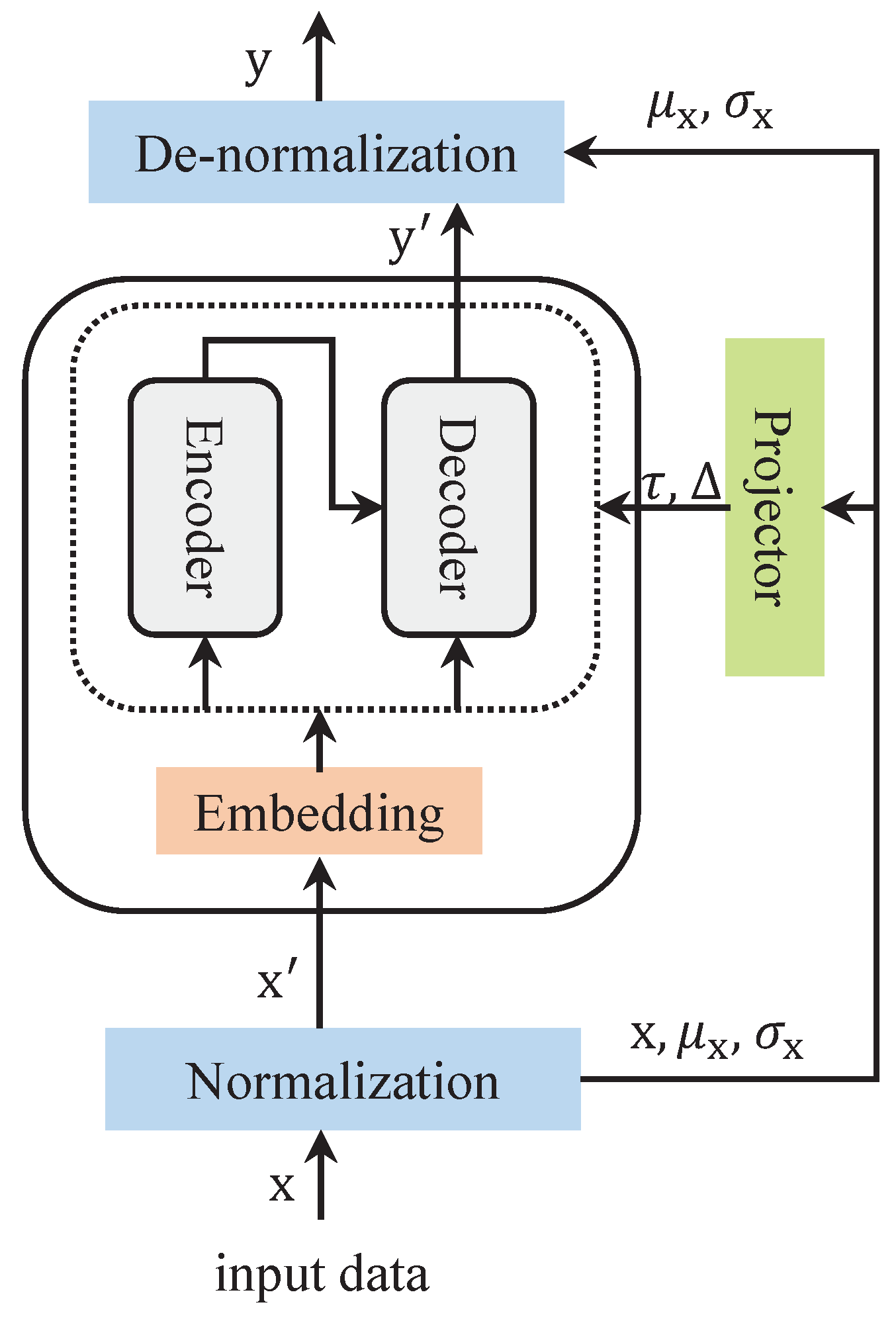
As shown in Figure 1, a normalization module and a de-normalization module perform the processing of the input and output data, respectively. By transforming the sequence data with these two modules, the model maintains better predictability. It is assumed that the input data are processed as , where L and N denote the input data length and number of variables. The formula can be expressed as follows:
where , , denotes the element-wise division, and ⊙ denotes the element-wise product.
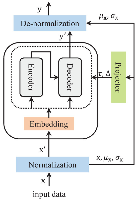
Figure 1.
The architecture of the Series Stationarization module.
It is assumed that the length of the prediction is S and the output data . Processing through the de-normalization module results in . The formula can be expressed as follows:
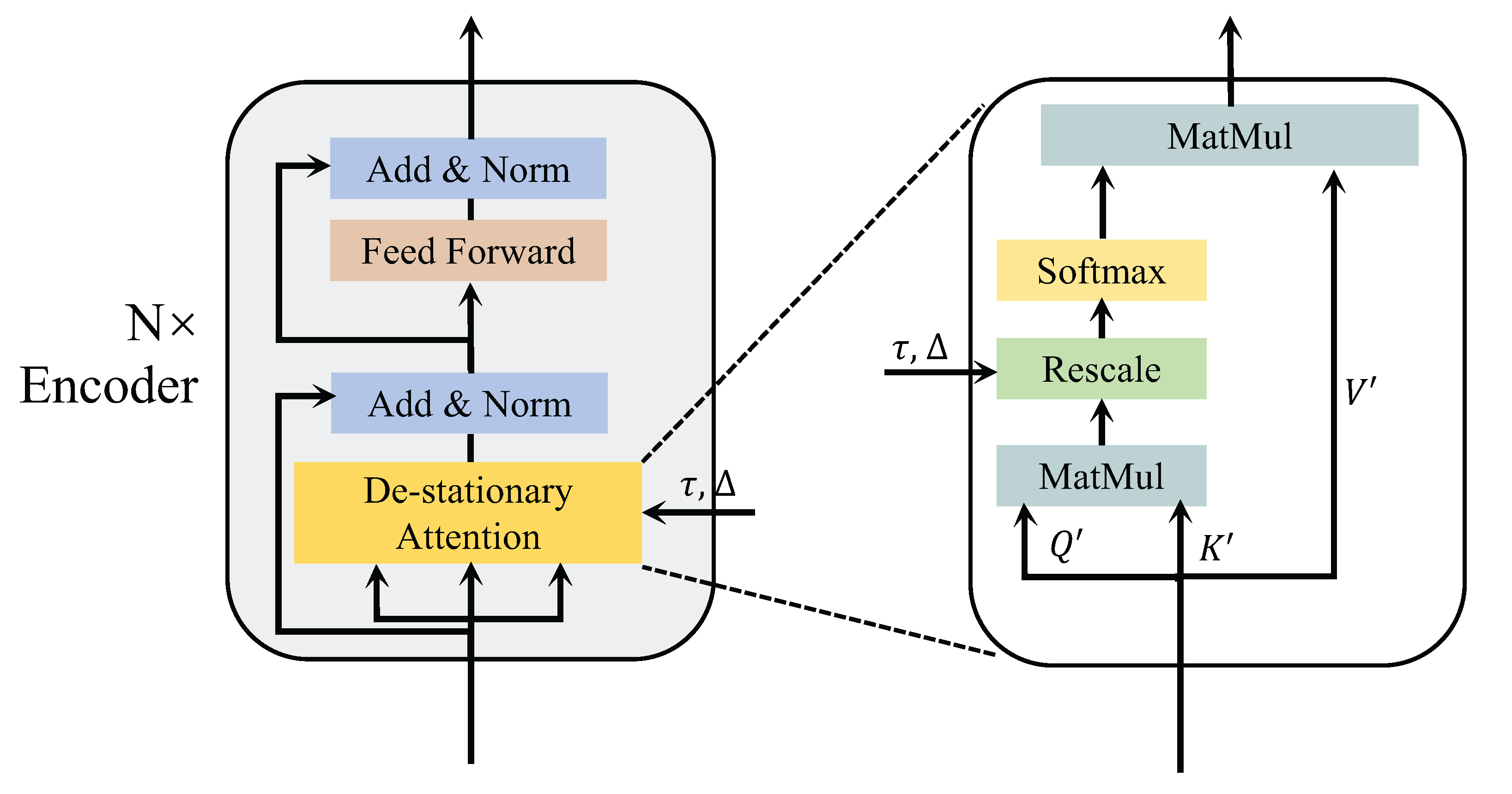
3.2.2. De-Stationary Attention
This section introduces an improved attention mechanism to better capture temporal dependencies in non-stationary time series data. The architecture of the modified attention mechanism is illustrated in Figure 2.
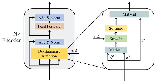
Figure 2.
The architecture of the De-stationary Attention.
The model receives the normalized input and subsequently computes the new , , . The query is represented as , where denotes feedforward layer, and is an all-one vector. The transformations of and are similar to . Then, a multilayer perceptron is used to learn the de-stationary factors , from the statistics , and of the unstationarized original time series . Finally, the new formula for attention is as follows:
where and represent the positive scale scalar and shifting vector. Now, the attention mechanism combines the information of the original series with the attention information of the stationarized series. It can improve the predictability of the non-stationary series while maintaining the temporal dependencies of the original series.
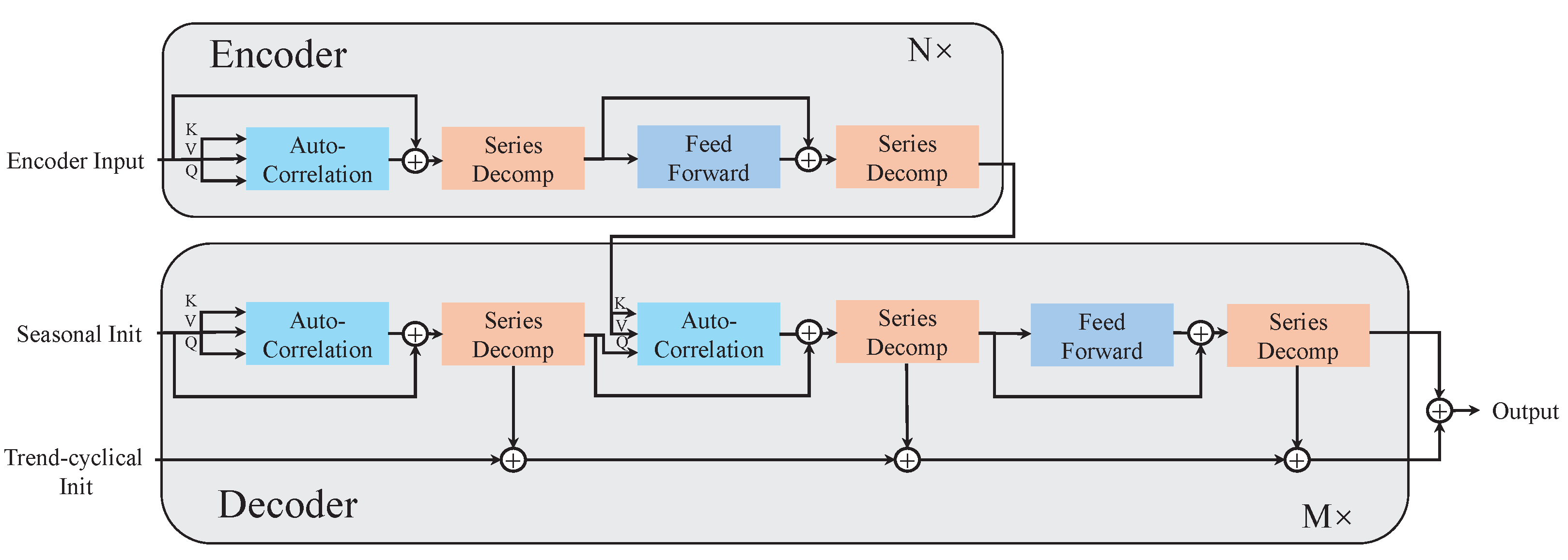
3.3. Autoformer
The Autoformer enhances the Transformer architecture by introducing a novel self-attention mechanism, improving both computational efficiency and forecasting accuracy [21]. It employs an Auto-Correlation mechanism to identify dependencies across series and effectively aggregate information, capturing both local and global patterns. It integrates time series decomposition with a progressive decomposition module to overcome limitations of traditional preprocessing-based methods. The model consists of three core components: Decomposition Block, Auto-Correlation Mechanism, and Encoder–Decoder Architecture. Its structure is illustrated in Figure 3.
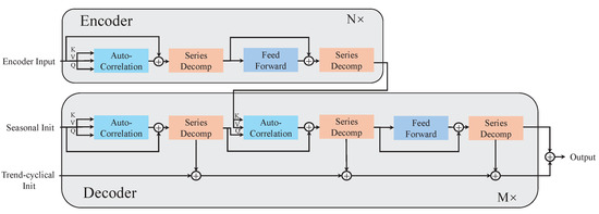
Figure 3.
The architecture of the Autoformer.
3.3.1. Decomposition Block
The Autoformer model’s series decomposition block splits time series into trend and seasonal components. The block maintains time series length with padding and extracts seasonal terms by subtracting trend terms. To effectively extract the trend information, a moving average method is used. For series of length L, the processing results in the following series:
where denote the seasonal part and the extracted trend part, respectively. The equation is summarized by .
The inputs to the encoder are series of length I time steps in the past, and the input to the decoder consists of a seasonal part and a trend part , O denotes the padding length serving as a placeholder for future predictions.
where and represent the seasonal and trend-cyclical components of respectively. The matrices and are placeholder sequences filled with zeros and the mean value of respectively.
3.3.2. Encoder and Decoder
The encoder module is concerned with the modeling of the seasonal part, and the output contains the past seasonal information, which will be used as mutual information to help the decoder adjust the forecasting results. Assuming we have N encoder layers, the l-th encoder layer has the following internal structure:
where “−” is the portion of the trend that was excluded. denotes the output of the l-th encoder layer, and is the embedded . denotes the seasonal component after the i-th series of the decomposition block in the l-th layer. Finally, here replaces self-attention.
The decoder consists of two parts: a cumulative operation for trend components and a stacked autocorrelation mechanism for seasonal components. Assuming that there are M decoding layers, using the latent variables from the encoder, the equations for the l-th decoder layer can be summarized as . The internal details are as follows:
where denotes the output of the l-th decoder layer. embedding from is used for deep transform and is used for accumulation. denote the seasonal component and the trend component following the i-th series of decomposition block in l-th layer, respectively. denotes the i-th extracted trend of the projection layer. Finally, the predicted value, as , is obtained from the sum of the two decomposition components, where projects the seasonal component of the deep transformation to the target dimension.
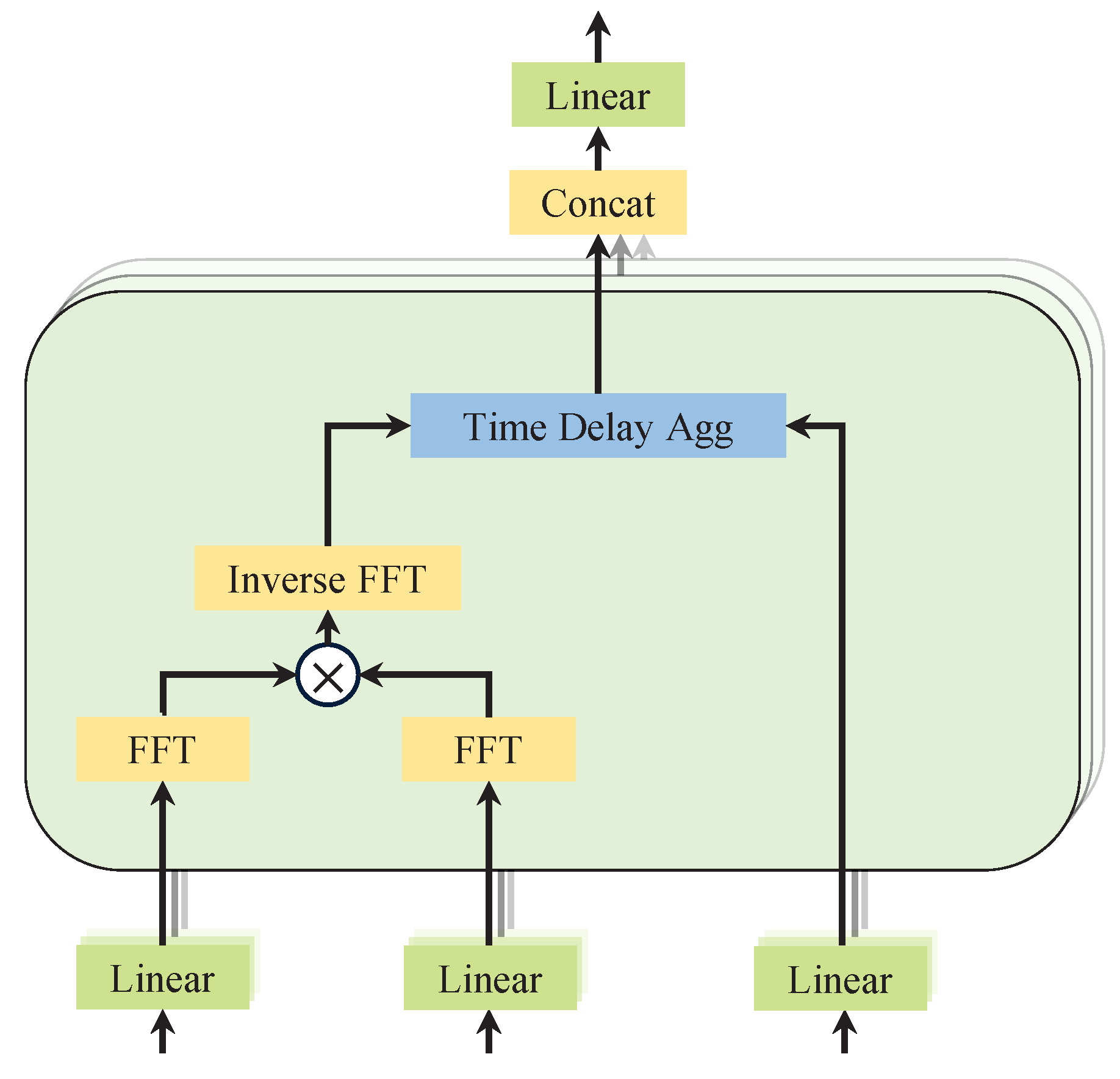
3.3.3. Autocorrelation Mechanism
The autocorrelation module, as demonstrated in Figure 4, is designed to identify period-based dependencies. It achieves this by calculating the autocorrelation coefficients of the series. Then, it rolls the series to perform time-delay aggregation of similar sub-series. The correlation between the original series and its lagged series is calculated. This helps identify periodically similar sub-series.

Figure 4.
Diagram of autocorrelation mechanism.
For a real discrete-time process , the autocorrelation can be obtained by the equation. It quantifies the time-delay similarity between and its lagged counterpart . By selecting the top-k delays with the highest autocorrelation scores, dominant periodic patterns in the sequence can be identified. To utilize these patterns, a time-delay aggregation mechanism is used to aligns sub-series at the same phase positions across the estimated periods. Unlike conventional dot-product attention, this method explicitly captures periodic dependencies and performs weighted aggregation using softmax-normalized autocorrelation scores.
For the single-head case and time series of length L, after the projection layer (projector), the query , the key , and the value can be obtained. Thus, it can seamlessly replace the self-attention mechanism.
where in the operator, and c is the hyperparameter. The autocorrelation between the series and is denoted as . is an operation on with time delay , and the element moved out of the first position will be reintroduced in the last position. In the encoder–decoder autocorrelation, and come from the encoder and are resized to length O. is from the previous block of the decoder.
In order to improve the computational efficiency, the model is based on the Winer–Khinchin theory and the autocorrelation coefficients are computed using the Fast Fourier Transform (FFT):
where , denotes the FFT, and * denotes the conjugate operation. This is achieved by converting the signal to frequency and then calculating through the frequency domain.
3.4. Non-Stationary Autoformer
Non-stationary Autoformer is a novel architecture designed for non-stationary time series forecasting. It extends the Autoformer backbone by incorporating key components from the Non-stationary Transformers framework.
Compared to Autoformer, NSAutoformer introduces a normalization-based preprocessing module. This module stabilizes the input distribution by extracting the mean and standard deviation of the input sequence. These statistics are subsequently fed into multilayer perceptrons to produce two learnable de-stationary factors: a global scaling factor () and a temporal shifting vector (). These de-stationary factors are then injected into the autocorrelation mechanism to modulate temporal dependency modeling.
Instead of directly relying on raw autocorrelation values, De-stationary autocorrelation modulates the correlation scores using these adjustment factors. This design allows the model to better capture evolving patterns and distributional shifts over time. The time-delay aggregation process follows that of Autoformer. NSAutoformer integrates non-stationary-aware attention with the efficient autocorrelation structure. At the same time, it significantly improves robustness to time-varying distributions.
By integrating these modules, NSAutoformer enhances the adaptability of the baseline to non-stationary environments. It retains the ability to model trend and seasonal components through decomposition. As a result, the model can better capture complex, time-varying dynamics in real-world time series. It ensures stable and accurate forecasting of non-stationary data across domains such as finance, energy, and macroeconomics.
3.5. Sentiment Analysis
In finance, sentiment analysis is primarily conducted using sentiment dictionaries, machine learning, and deep learning [40,41]. Sentiment dictionaries offer a straightforward and efficient method for analyzing financial texts rich in domain-specific terms. As our experiments used unlabeled social media texts, sentiment dictionaries were a suitable choice. They do not require labeled data, thus reducing both time and cost. Moreover, investor comments tended to be consistent and repetitive, allowing a fixed vocabulary list to classify sentiments effectively with low computational cost.
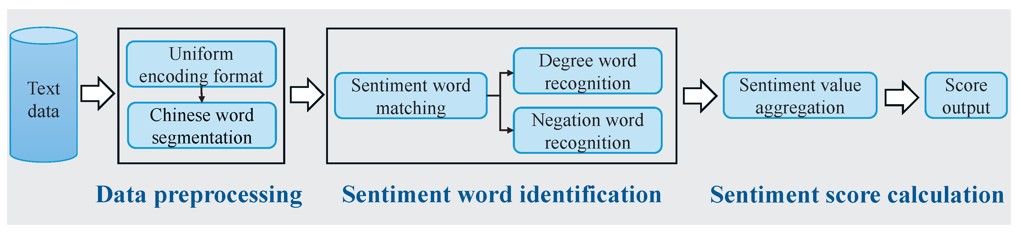
To improve sentiment analysis, we developed a financial sentiment dictionary by extending an existing lexicon to better capture financial terms and sentiment nuances. The processes of sentiment categorization and feature construction are illustrated in Figure 5.

Figure 5.
A dictionary-based method for financial sentiment analysis in Chinese.
3.5.1. Construction of Financial Sentiment Dictionary
We integrated two Chinese financial sentiment dictionaries developed by Jiang Fuwei and Yao Jiaquan to construct an enhanced lexicon [42,43,44]. Their original dictionaries were built using data mining and deep learning techniques to analyze both formal sources (e.g., annual reports) and informal sources (e.g., social media data). The formal sentiment dictionary categorized annual reports as positive or negative based on cumulative stock returns within three trading days of release. Investor posts from A-share companies on Xueqiu and Eastmoney were analyzed to extract market sentiment from informal sources.
3.5.2. Sentiment Index Calculation
In this study, investor posts from social platforms were transformed into sentiment scores using the constructed dictionary. The computation process begins with segmentation and lexical labeling of Chinese sentences, followed by sentiment word extraction. Sentiment words such as increase, bullish, and optimistic are assigned a score of +1, whereas negative words like decline, bearish, and pessimistic are assigned a score of –1. If a sentiment word is preceded by a degree adverb or a negation, its score is multiplied by the corresponding weight. Degree adverbs are weighted as follows: extreme = 4, very = 3, more = 2, and ish = 1. A negation word, such as not or never, is assigned a weight of −1. This process continues sequentially until the entire text is processed. Finally, the scores for all words in a sentence are summed to generate the final sentiment score.
Example 1
(Positive Comment). “The market is very bullish today and expected to rise further”.
- The word bullish is a positive sentiment word (), preceded by the degree adverb very: (weight = 3) → score = .
- The word rise is a positive sentiment word (), with no modifier → score = .
- Final sentiment score: .
Example 2
(Negative Comment). “The outlook is not optimistic and prices may slightly decline”.
- The word optimistic is a positive sentiment word (), but is preceded by the negation not: (weight = ) → score = .
- The word decline is a negative sentiment word (), preceded by the degree adverb slightly: (weight = 1) → score = .
- Final sentiment score: .
The daily sentiment index, serving as a proxy for investor sentiment, is computed as the average sentiment score across all posts on a given day, where i represents the i-th post, and n denotes the total number of posts.
The same method was applied to compute sentiment scores for financial news. Long articles were split into sentences, which were analyzed sequentially and aggregated into an overall sentiment score. Due to their length, news articles may exhibit inflated sentiment scores. To mitigate this effect, each article was classified as positive, negative, or neutral based on its aggregated score. The calculation formula is as follows:
where and denote the number of positive and negative news articles for the day, respectively.
3.6. Forecasting Framework
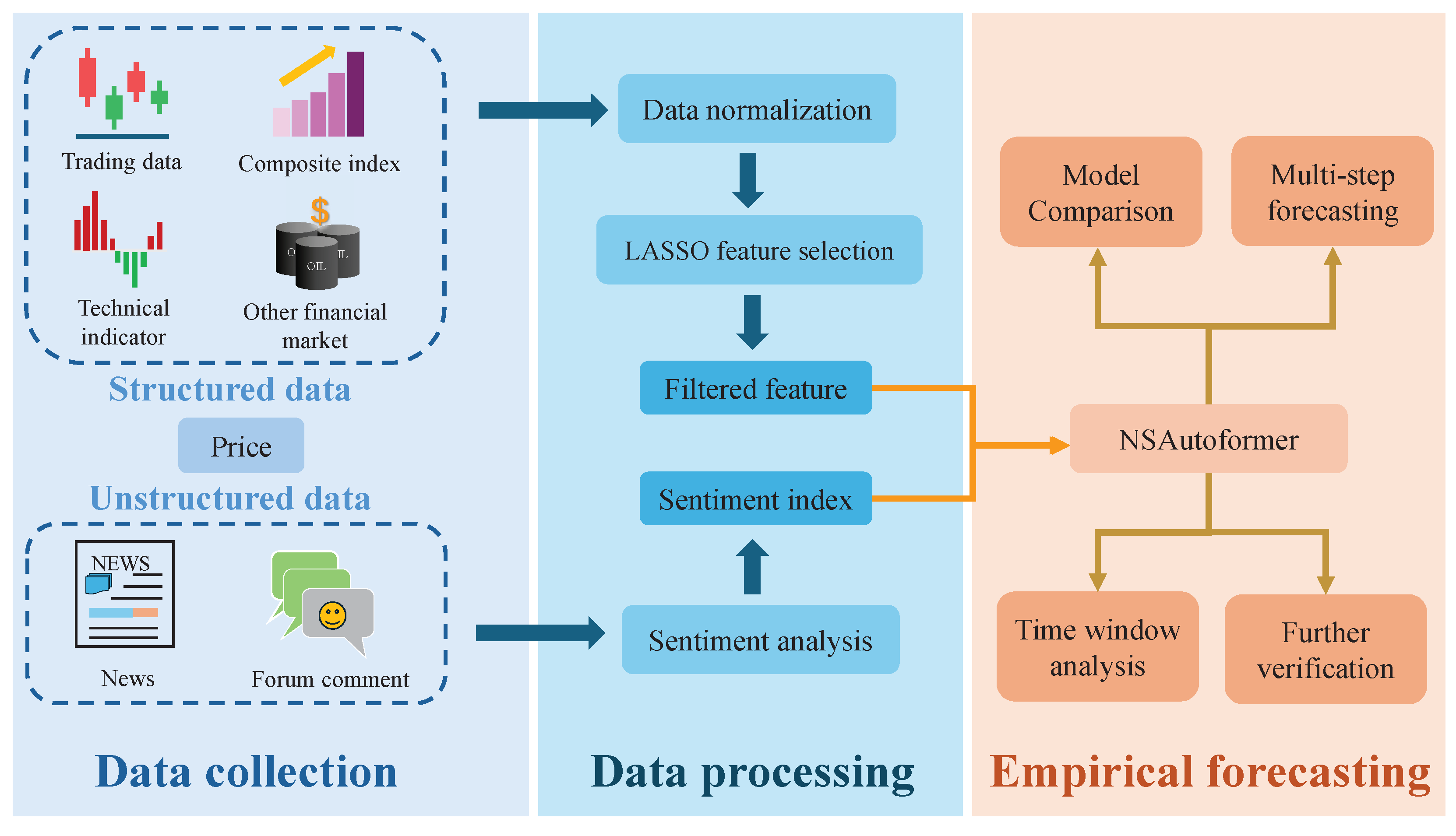
To capture complex market behaviors, we designed LASSO-NSAutoformer, a hybrid model integrating feature selection, sentiment analysis, and deep learning. It combines filtered structured features and sentiment signals from unstructured text to form a unified forecasting input. This integration enables a comprehensive representation of market dynamics. As illustrated in Figure 6, the proposed method consisted of three main stages: data collection, data processing, and empirical forecasting.
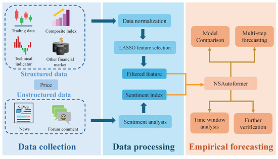
Figure 6.
Hybrid forecasting framework.
Step 1: Data collection. Factors were collected from various domains and categorized into structured and unstructured sources. Structured data included historical price series, trading data, technical indicators, composite indices, and other financial market variables. Unstructured data consisted of investor comments and financial news.
Step 2: Data processing. Structured variables were preprocessed, and LASSO was applied to select key features, reducing redundancy. For unstructured text, sentiment scores were computed using a domain-specific financial sentiment dictionary, yielding investor and news sentiment indices. These indices were combined with LASSO-selected features to form the final model input.
Step 3: Empirical forecasting. The combined input was fed into NSAutoformer. Several comparative experiments were conducted across different feature sets, selection methods, and forecasting models to evaluate the robustness and accuracy of the proposed approach. Additionally, sensitivity tests on time window lengths and forecast horizons were performed to assess stability.
3.7. Evaluation Metrics
To evaluate the model’s forecasting accuracy, we used four standard regression metrics: MAE, RMSE, MAPE, and R2:
where is the predicted value, is the true value, is the average of , and n is the sample size. MAE measures the average absolute error, while RMSE reflects error magnitude in the same units as the target. MAPE expresses the average percentage error, and R2 quantifies the proportion of variance explained by the model.
4. Experiments
4.1. Data Preparation
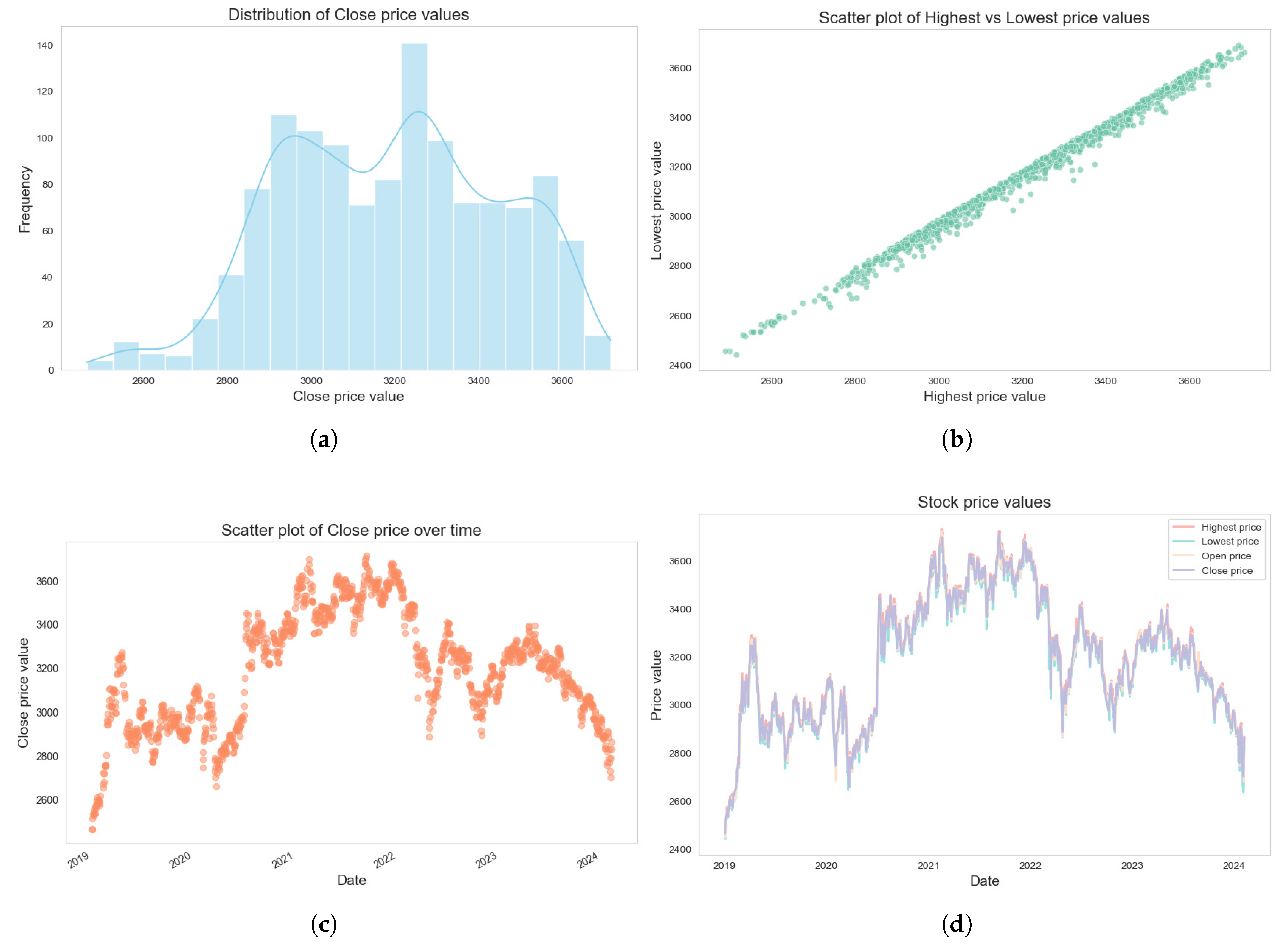
In experiments, we found that individual stocks are more volatile due to firm-specific or industry factors, while market indices are better suited for research [45]. To ensure representativeness, we selected the Shanghai Securities Exchange Composite Index (SSECI), which includes all A-share stocks on the Shanghai Stock Exchange (SSE) and covers a wide range of industries, making it the most comprehensive stock index in China’s financial market. Table 1 shows a sample of SSECI price and trading data, obtained using the efinance package in Python 3.13.2 [46]. The dataset spans from 2 January 2019 to 8 February 2024. Figure 7 illustrates an exploratory analysis of SSECI price trends.

Table 1.
Data samples of the SSECI.

Figure 7.
Data analysis of the SSECI. (a) Distribution of close price. (b) Scatter plot of highest vs. lowest price. (c) Scatter plot of close price over time. (d) Stock price values.
We used TA-Lib (Technical Analysis Library) to calculate 28 commonly used technical indicators based on price and trading data. Details are listed in Table 2. Trend indicators identify market direction—uptrend, downtrend, or consolidation [47]. Momentum indicators measure price movement speed, detecting overbought or oversold conditions. Volume indicators assess trend strength and market interest through trading volume changes.
Table 2.
Calculated technical indicators.
In addition, we selected 12 variables categorized into two groups: (1) Composite indices: Daily Geopolitical Risk Index (GPRD), Daily Infectious Disease Equity Market Volatility Index (IDEMVI), search volume on Google Trends (GT), and Baidu Index (BI). (2) Other financial markets: COMEX gold futures closing price (GC), West Texas Intermediate (WTI), Dow Jones Industrial Average (DJIA), NASDAQ Composite Index (NASDAQ), S&P 500 Index (S&P), USD to CNY Exchange Rate (USDCNY), U.S. Dollar Index (DXY), and HANG SENG INDEX (HSI). Table 3 summarizes the details of these two categories.
Table 3.
Selected variables within two categories.
In the composite index, we considered the impact of geopolitics and COVID-19 on the stock market. The GPRD [48] reflects a measure of geopolitical events and associated risks, based on newspaper statistics. Prior studies have shown that wars and crises typically reduce investment, depress stock prices, and lower employment, indicating a strong link between geopolitical risks and economic performance. The IDEMVI [49] captures the relationship between infectious disease outbreaks and equity market volatility, particularly during the COVID-19 period. GT [50] and BI [51] represent search activity on Google and Baidu, the largest search engines globally and in China, respectively. These indices reflect keyword search volumes and serve as proxies for market attention and interest preferences.
In recent years, globalization and financial integration have strengthened linkages among regional markets. Correlations and risk spillovers across markets have attracted significant scholarly attention, particularly during crises when such linkages intensify. Asset price movements often propagate across markets, forming a complex network of interdependencies. All variables related to other financial markets were obtained using the efinance package.
In summary, 49 candidate variables were collected for structured data. Regarding unstructured text data, investor comments were collected from the Eastmoney Guba forum [52] as shown in Table 4. Financial news was sourced from China News [53] (A-share section) and macro/news finance columns on China.com.cn [54]. Additional policy-related content, including current affairs, key events, press conferences, and policy interpretations, was collected from the official website of the China Securities Regulatory Commission (CSRC) [55]. All text data were obtained using the Bazhuayu web crawler [56], covering the period from 2 January 2019 to 8 February 2024 [57].
Table 4.
Sample text data from investor forum.
4.2. Data Preprocessing
The dataset was divided into training (70%), validation (10%), and test sets (20%). Prior to experimentation, data normalization was applied to ensure numerical stability and feature comparability. Each feature was standardized by computing its mean and variance independently. The formula is as follows:
where denotes the original data, denotes the mean of the data, denotes the standard deviation of the input data, and denotes the standardized result.
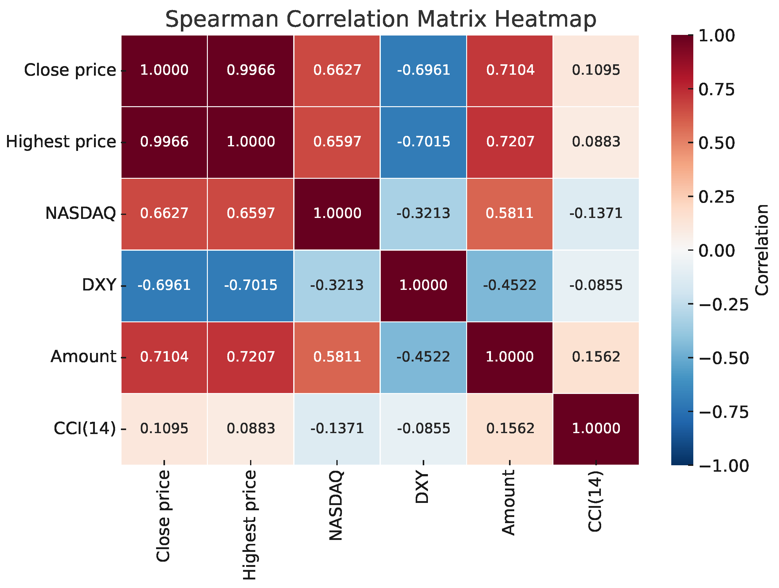
Excessive features can hinder model efficiency and forecasting accuracy, so LASSO was applied for feature selection by compressing some coefficients to zero. The LASSO model was optimized using grid search and 10-fold cross-validation, resulting in features with thresholds greater than zero, as shown in Table 5. Spearman correlations among the selected features are shown in Figure 8.
Table 5.
Results of the LASSO feature selection.

Figure 8.
Spearman correlation matrix heatmap.
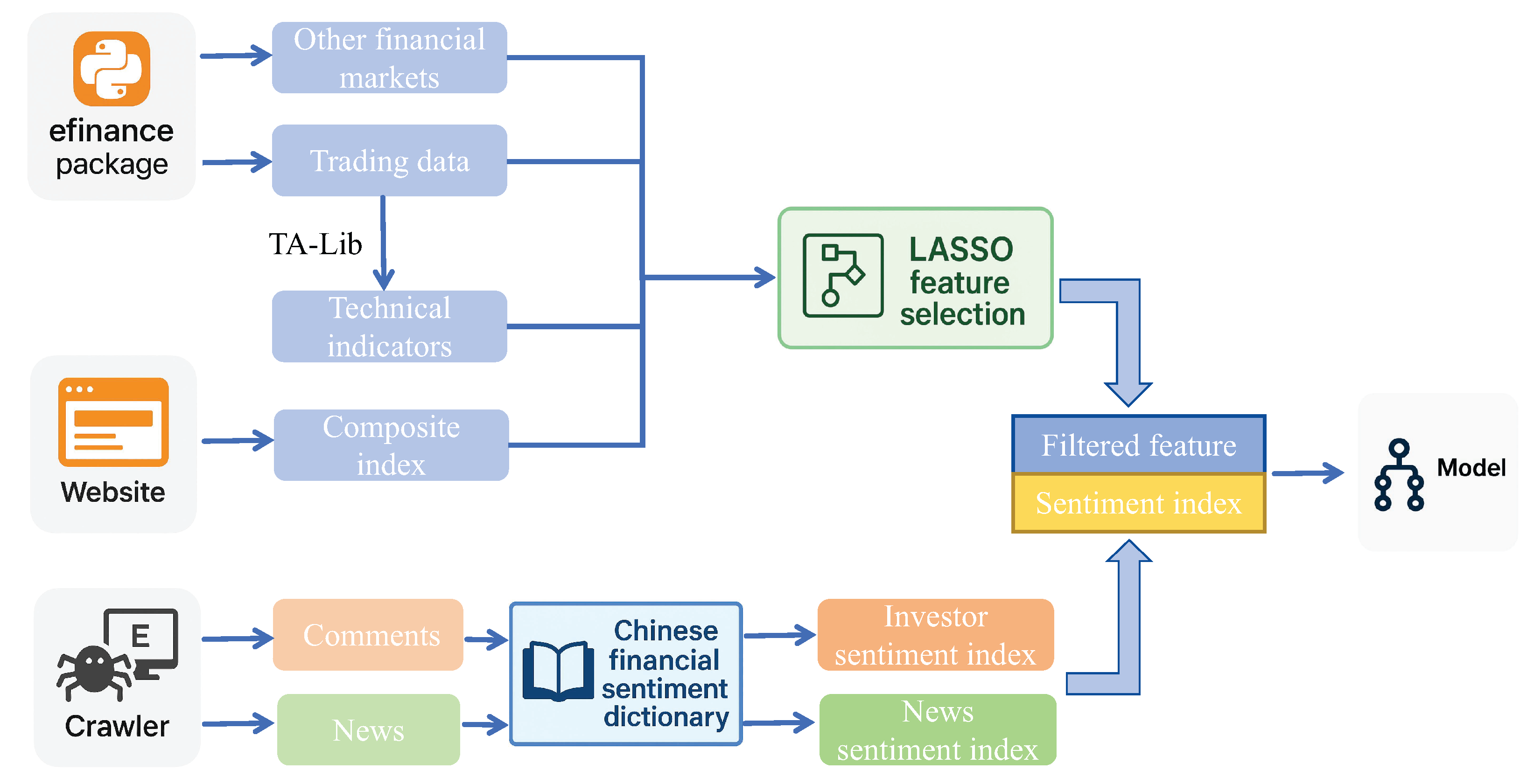
For text data, we applied the constructed Chinese financial sentiment dictionary after preprocessing to extract investor and news sentiment indices. To minimize the impact of extreme values, obvious outliers were removed. In total, 4,529,650 valid comments were retained. Figure 9 illustrates the complete data processing pipeline, from raw data acquisition to the construction of model input features.

Figure 9.
The full pipeline of the proposed forecasting framework.
4.3. Hyperparameters Setting
Hyperparameter tuning was performed using Optuna, which applies Bayesian optimization with a Tree-structured Parzen Estimator (TPE) to efficiently search the parameter space. The framework minimizes validation loss across multiple trials and selects the best configuration accordingly. Table 6 defines the search space and Table 7 reports the optimal hyperparameters for each model. Mean absolute error (MAE) was used as the loss function. Training was conducted for up to 50 epochs with early stopping to prevent overfitting and ensure convergence.
Table 6.
Hyperparameter search space.
Table 7.
Optimal parameters for each model.
5. Results and Analysis
We adopted the moving window approach, a common method in time series forecasting. This approach uses a sliding window over the data, allowing the model to generate predictions at each time step. In our experiment, features from the trading day T were used to predict the price on the following day, .
5.1. Feature Set Evaluation
Given the inclusion of multiple data sources, we conducted an experiment to evaluate the predictive performance of different feature sets. Table 8 presents the results of five candidate variable sets using the proposed NSAutoformer. The results show that adding technical indicators, composite indices, and financial market data to the base set reduces forecasting errors and improves accuracy. This indicates that incorporating a wider range of relevant features can enhance price forecasting capability. Notably, the lowest MAE was observed in , which includes price, trading, and technical indicators, confirming the positive impact of technical factors. However, when all variables are included (), performance declines, indicating that excessive features may introduce noise and increase overfitting risk. To mitigate this, we apply the LASSO algorithm for feature selection.
Table 8.
The prediction performance of different feature sets.
Subsequently, we constructed new feature sets by combining the LASSO-filtered variables with sentiment indices. As shown in Table 9, , which contains only the filtered features, outperforms all raw feature sets (Sets 1–5), indicating that LASSO improves model accuracy by removing irrelevant or noisy variables. Compared to the best raw set (), reduces MAE from 20.718376 to 20.350271 and increases R2 from 0.967436 to 0.970052.
Table 9.
The prediction performance of combined filtered features and sentiment factors.
Furthermore, incorporating sentiment indices (Sets 7–9) improved model performance. The best result occurred when both investor and news sentiment were included, yielding the lowest MAE (19.253584) and highest R2 (0.972357). These findings confirm the complementary benefits of feature selection and sentiment integration. LASSO reduces redundancy, while sentiment indices capture psychological factors often missing from traditional financial features.
The consistent improvement suggests that psychological factors significantly influence market dynamics. Integrating sentiment from multiple sources improves index prediction, with broader group sentiment yielding better results. Investor sentiment reflects short-term fluctuations driven by individual behavior, while news sentiment captures broader market tone and policy direction. Together, these two sentiment sources provide complementary information. These findings further support integrating sentiment analysis into the forecasting framework, allowing the model to adapt to dynamic market conditions.
We also compared several feature selection algorithms, including XGBoost, Random Forest, CatBoost, and AdaBoost, which are widely used in machine learning. To ensure fairness, model structures and hyperparameter tuning followed settings from relevant studies. As shown in Table 10, all algorithms improved forecasting accuracy, with LASSO achieving the lowest error and best overall fit.
Table 10.
Comparative experiment applying different feature selection algorithms.
Among the feature selection methods compared, LASSO-filtered features achieved the best forecasting accuracy. Unlike ensemble-based methods like Random Forest or XGBoost, which tend to produce dense feature sets requiring extra tuning, LASSO yields sparse and interpretable models with fewer variables. This aligns with the goals of economic and financial forecasting, where transparency and stability are essential. Moreover, its simplicity, computational efficiency, and robustness to multicollinearity make LASSO well suited for high-dimensional financial time series.
5.2. Forecasting Results
This section presents comparative experiments evaluating different forecasting models on the SSECI dataset. The evaluation focuses on one-step forecasting, with results reported using MAE, RMSE, MAPE, and R2, as shown in Table 11. The results reveal a clear pattern: advanced model architectures generally yield better predictive performance. In particular, Transformer-based models consistently outperform RNN-based models, with NSAutoformer delivering the most accurate results overall.
Table 11.
Forecasting error of single models.
The performance of the basic RNN model is the weakest, underscoring its limitations in capturing long-range dependencies and handling high-dimensional feature inputs. Although GRU (MAE: 34.960663, RMSE: 47.148529, MAPE: 0.011468, R2: 0.905338) and LSTM (MAE: 35.166011, RMSE: 47.015923, MAPE: 0.011536, R2: 0.905870) improve upon RNN, they remain inferior to their bidirectional versions and Transformer-based models.
The vanilla Transformer (MAE: 35.786094, RMSE: 43.768764, MAPE: 0.011411, R2: 0.918423), while more effective than RNN-based models, was surpassed by its enhanced variants. Informer (MAE: 33.746243, RMSE: 43.102985, MAPE: 0.010937, R2: 0.920886) improved accuracy through the ProbSparse self-attention mechanism, which reduces computational cost by focusing on dominant queries. Autoformer further improved forecasting by decomposing time series into trend and seasonal components.
Among Transformer-based models, the proposed NSAutoformer is built on the Autoformer architecture. It incorporates non-stationary modeling to improve adaptability to dynamic data distributions. It adapts the autocorrelation mechanism to handle distributional shifts, improving ability to represent complex, evolving temporal patterns. Without relying on feature selection or sentiment inputs, NSAutoformer already achieved the best results across all metrics (MAE: 21.098995, RMSE: 27.456692, MAPE: 0.006787, R2: 0.967898). These results demonstrate NSAutoformer’s architectural advantage in capturing both structural and statistical complexity, highlighting the importance of models tailored to non-stationary time series forecasting.
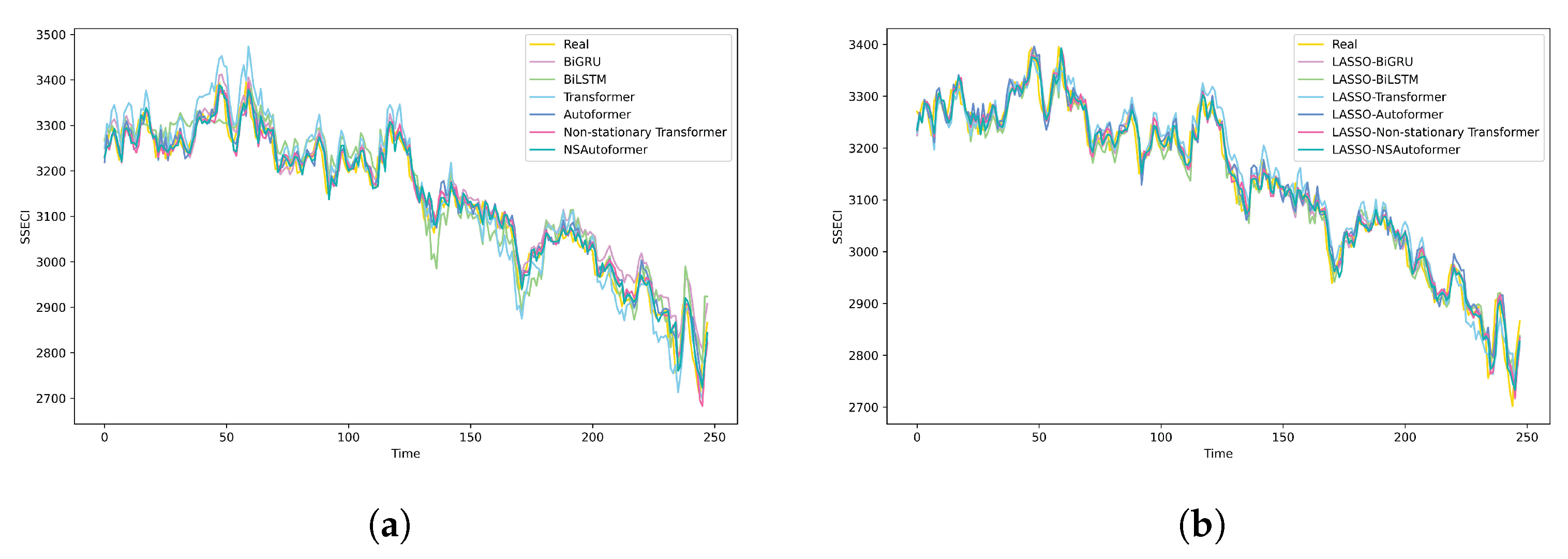
Building on the single-model results, we evaluated a hybrid forecasting framework that integrates LASSO-based feature selection and sentiment analysis. As shown in Table 12 and Figure 10, incorporating filtered features and sentiment indices significantly reduced MAE, RMSE, and MAPE values, while consistently improving R2. These results highlight the benefit of combining data-driven feature selection with sentiment inputs, which together enrich the input space.
Table 12.
Forecasting error of hybrid forecasting models.
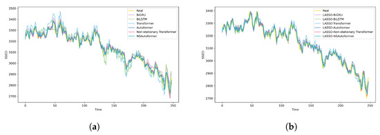
Figure 10.
Comparison of fitting curves of different forecasting models. (a) Single model. (b) Hybrid model.
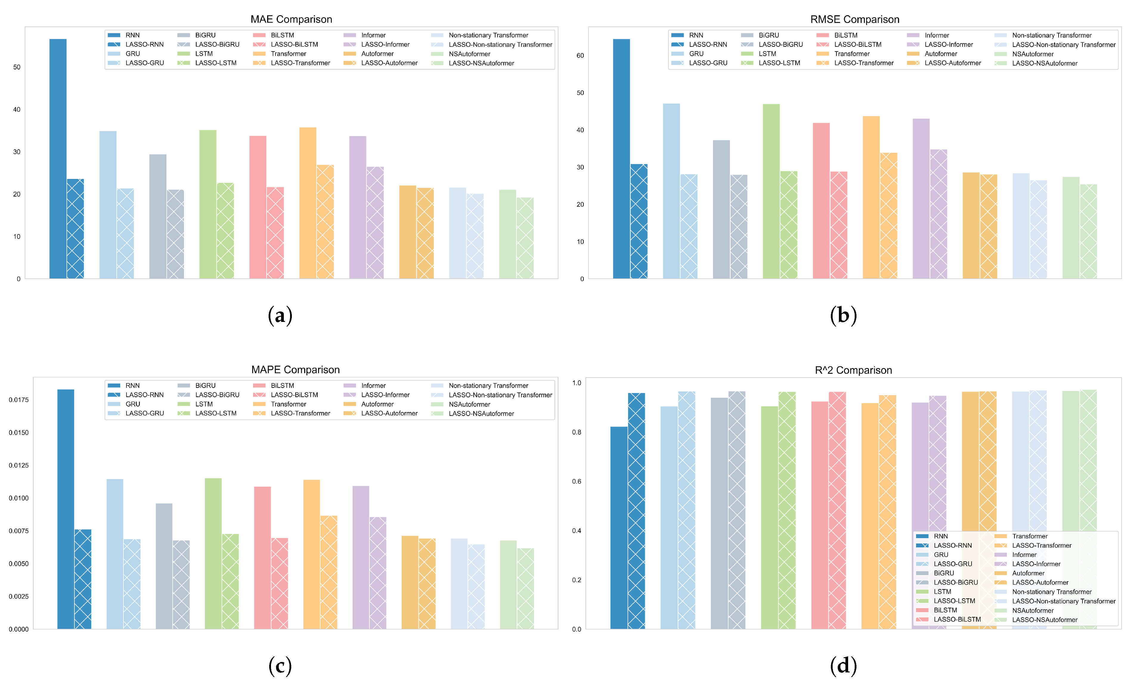
Notably, the hybrid model reduced MAE by 58.28%, 38.82%, 28.31%, 35.42%, 35.71%, 24.65%, 21.44%, 2.57%, 6.75%, and 8.75% relative to individual baseline models. These results clearly demonstrate the advantage of the proposed framework over individual models. Figure 11 further illustrates forecasting performance across all metrics, highlighting the superiority of the hybrid approach.
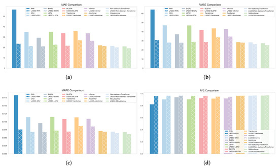
Figure 11.
The forecasting model’s predictive performance is evaluated across four metrics. (a) MAE. (b) RMSE. (c) MAPE. (d) R2.
However, within the hybrid models, Transformer and Informer underperformed compared to RNN. This may be due to their architectural complexity: although effective in high-dimensional settings, they require large datasets and rich feature representations to perform optimally. In contrast, LASSO reduces dimensionality, potentially limiting these models’ capacity to capture nonlinear interactions. As a result, they become less effective than RNN-based models when inputs are simplified. This finding aligns with machine learning theory, which suggests simpler models often generalize better with limited input spaces.
Among all hybrid configurations, LASSO-NSAutoformer achieved the best performance (MAE: 19.253584, RMSE: 25.478617, MAPE: 0.006189, R2: 0.972357). These results provide strong empirical support for the proposed framework, highlighting both its architectural advantage and its effectiveness in integrating heterogeneous data sources to enhance predictive accuracy.
5.3. Multi-Step Forecasting Evaluation
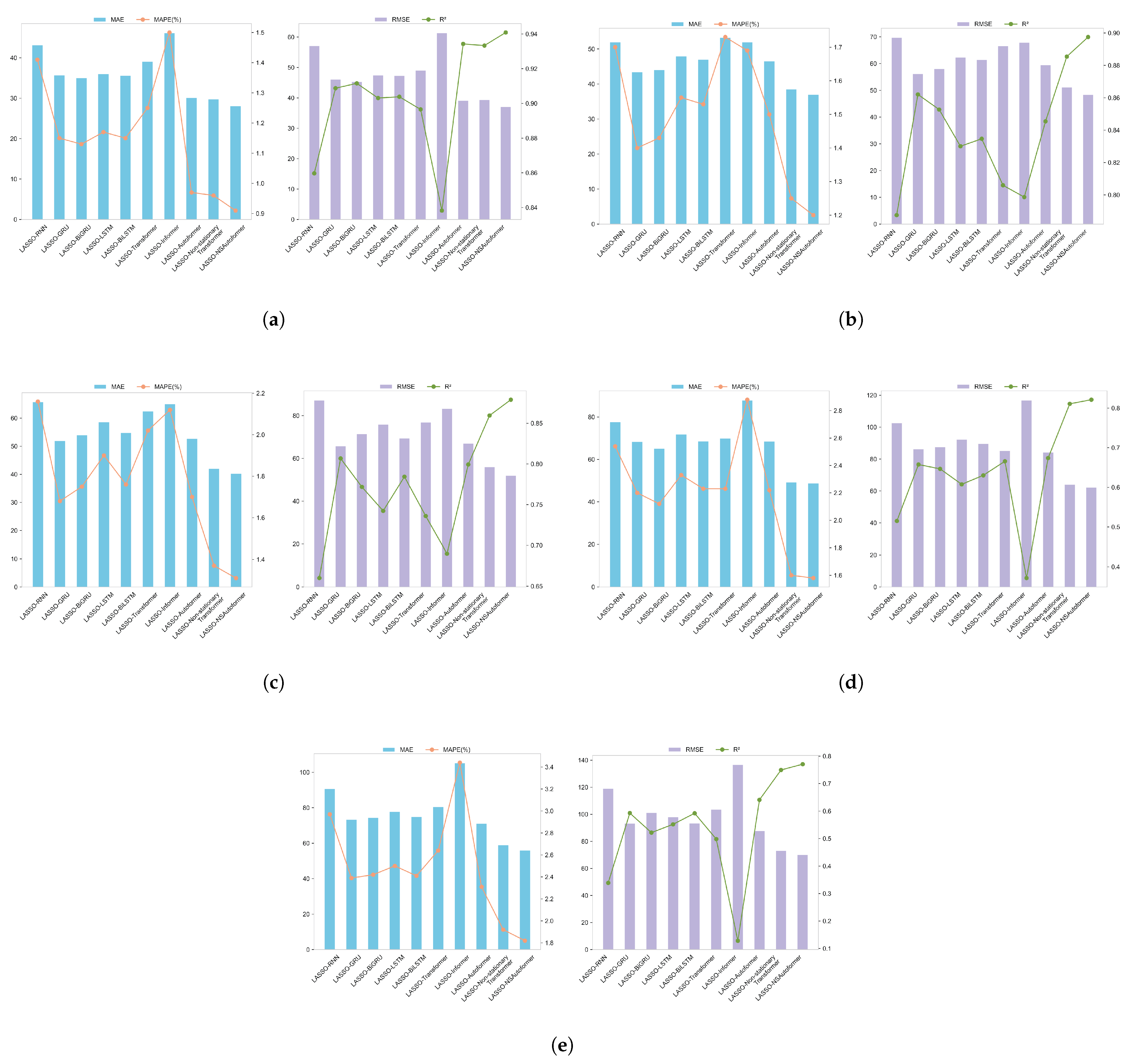
To assess the model’s temporal scalability, we conducted multi-step forecasting using a moving window across horizons of 3, 5, 7, 10, and 12 steps. This setup enables comprehensive evaluation across short-, medium-, and long-term forecasting tasks. Table 13 presents the error metrics for each forecast horizon, followed by an analysis of performance variation across temporal scales. Figure 12 visually compares the prediction results of different models across various forecasting horizons.
Table 13.
Evaluated performance of multi-step forecasting.

Figure 12.
Multi-step forecasting performance of different models. (a) Three-step. (b) Five-step. (c) Seven-step. (d) Ten-step. (e) Twelve-step.
The multi-step forecasting results provide strong evidence for the effectiveness of LASSO-NSAutoformer, particularly in terms of accuracy and stability across different horizons. Specifically, it achieved the lowest MAE and MAPE in short-term (three-step: MAE 28.095316, MAPE 0.009050) and medium-term forecasts (five-step: MAE 37.026203, MAPE 0.011978), significantly outperforming other models. These results confirm the model’s strong ability to capture market dynamics, which is essential for financial forecasting.
As the forecasting horizon increased to 7, 10, and 12 steps, all models showed reduced accuracy. However, LASSO-NSAutoformer consistently maintained the lowest errors and showed slower performance degradation than other models. This stability across longer horizons highlights the model’s adaptability to evolving market dynamics and supports its application in long-term forecasting. In practice, reliable multi-step forecasts help investors and portfolio managers anticipate future trends across various time horizons, enabling more informed decisions and effective risk management.
5.4. Time Window Analysis
The moving window approach is widely used in stock price forecasting, where window length is a critical parameter. It structures historical data into a format suitable for neural networks, directly influencing model performance. Generally, shorter windows capture short-term volatility but may miss long-term trends, while longer windows reduce noise but are less responsive to rapid changes. Thus, balancing short-term and long-term effects is key. Prior studies commonly use window lengths ranging from 5 to 30 days.
Table 14 shows model performance across window lengths from 5 to 30 days, evaluated using MAE, RMSE, MAPE, and R2. The results indicate that longer windows generally lead to higher error values and reduced model performance. Since the experiments focus on single-step forecasting, a window length of 5 to 15 days is optimal, with most models performing best at 10 days.
Table 14.
Time window length experiment.
As shown in Figure 13, LASSO-NSAutoformer consistently outperformed all other models across window lengths, with minimal performance degradation as the window increased. Its stable accuracy over longer historical spans suggests an effective balance between short-term fluctuations and long-term dependencies. This adaptability enhances the model’s practicality, enabling it to accommodate varying historical lengths common in real-world financial forecasting. Overall, the results confirm the framework’s strength in predictive stability and generalizability.
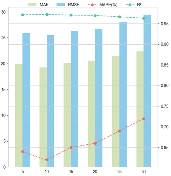
Figure 13.
The LASSO-NSAutoformer forecast results for different time window lengths.
5.5. Further Verification
To further validate the generalizability of our proposed forecasting approach, we conducted additional experiments on three Chinese stock indices: the Shenzhen Stock Exchange Composite Index (SZSECI), the Growth Enterprise Index (GEI), and the CSI 300 Index. Following the same methodology, structured variables and investor sentiment data were collected and processed. Sentiment indices were derived from 323,764 (SZSECI), 624,311 (GEI), and 39,488 (CSI 300) valid investor comments from related forums. These sentiment indices were combined with LASSO-selected variables to form the final input for model forecasting. The corresponding results are presented in Table 15.
Table 15.
Forecasting errors of models in other stock markets.
The proposed model showed stable and accurate performance across all three structurally distinct indices, rather than being effective in only one market condition. This consistency highlights the model’s ability to capture diverse market dynamics: SZSECI reflects overall market trends, GEI emphasizes volatile, growth-oriented stocks, and CSI 300 tracks stable, blue-chip firms. These indices differ in volatility, investor composition, and information sensitivity, offering a robust test for model adaptability. The model’s strong performance across all indices confirms its adaptability to varied financial environments.
Once again, integrating LASSO-selected features with sentiment analysis significantly improved forecasting performance across all models and indices. For instance, in the SZSECI, the MAE decreased from 98.346413 in the single Autoformer model to 94.025230 in the LASSO-enhanced Autoformer, eventually reaching an optimal value of 88.166016 in the LASSO-NSAutoformer. Similar improvements were observed for both GEI and CSI 300.
Overall, these findings demonstrate that the proposed framework is not only effective in a single setting, but also generalizes well to multiple market environments. Its consistent performance across structurally different markets suggests potential for broader application in financial forecasting tasks.
6. Conclusions
Stock market forecasting is a critical yet challenging task, primarily due to the volatility and non-stationarity of financial time series. This study proposes LASSO-NSAutoformer, a hybrid forecasting model for Chinese stock index that integrates multi-source data, LASSO feature selection, and deep learning. The framework consists of three components: (1) collecting 49 structured financial variables, with LASSO used to remove redundancy and retain key predictors; (2) constructing a Chinese financial sentiment dictionary to quantify market sentiment from investor comments and financial news; (3) integrating structured and sentiment-based features into a deep learning model that extends Autoformer to better capture non-stationary patterns.
This study conducts comparative experiments to evaluate the proposed framework. First, we examined the contributions of trading data, technical indicators, composite indices, and other market-related variables. Results showed that these variables contribute unevenly to prediction accuracy, highlighting the need to retain informative features and eliminate redundancy. Next, we evaluated the impact of sentiment by incorporating investor and news sentiment indices. These indices were derived from a domain-specific Chinese financial sentiment dictionary. Incorporating sentiment significantly improved forecasting accuracy, indicating that behavioral signals offer valuable information beyond traditional financial metrics. To optimize input features, we compared five selection algorithms (CatBoost, AdaBoost, XGBoost, Random Forest, and LASSO) and found LASSO consistently yielded the best results, supporting its use in the proposed framework.
To evaluate model effectiveness, we applied NSAutoformer to four major Chinese stock indices: SSECI, SZSECI, GEI, and CSI 300. In benchmark comparisons with nine deep learning models, NSAutoformer consistently achieved the best predictive performance, confirming its ability to capture complex temporal dependencies in financial time series. Building on this foundation, we developed LASSO-NSAutoformer, a hybrid model that integrates LASSO-based feature selection, sentiment analysis, and NSAutoformer. Compared to both single and hybrid baseline models, LASSO-NSAutoformer achieved superior results across all evaluation metrics. It also showed lower error growth and more stable performance across different forecast horizons and input window lengths. These findings demonstrate the model’s adaptability to dynamic and evolving market patterns, which is essential for practical stock index forecasting.
In summary, this study proposes and systematically validates a deep learning-based forecasting framework, demonstrating its effectiveness across multiple dimensions. First, the use of multi-source data provides a diverse set of predictors, enabling the model to capture complex market dynamics. Second, the integration of sentiment analysis allows the model to reflect investor responses and market tone. Third, LASSO-based feature selection enhances interpretability by identifying key predictors and reducing redundancy. Finally, the introduction of NSAutoformer yields superior predictive performance compared to existing models, confirming the reliability of deep learning in stock index forecasting.
By extracting sentiment from news, investor comments, and social media, the method helps assess market expectations and investor psychology. This approach is useful for individual investors, asset managers, and financial institutions. It shows the value of combining deep learning with sentiment analysis in financial forecasting and points to future directions for both research and practice.
Despite improved forecasting accuracy, several limitations remain. First, although the model integrates fundamentals, technical indicators, and sentiment, it excludes macroeconomic variables such as GDP growth, interest rates, and inflation expectations. Including these in future work may help capture macroeconomic cycles and enhance model interpretability. Second, the model is only validated on the Chinese stock market. Future research should extend it to developed markets and other asset classes (e.g., futures, bonds, foreign exchange). Third, the integration of feature selection, sentiment analysis, and deep neural networks may incur high computational costs, especially in large-scale applications. Future work should evaluate training and inference efficiency, and explore lightweight alternatives or model pruning. Finally, as stock indices are heavily influenced by a few high-weighted constituents, constructing features based on these components may enhance index-level forecasting accuracy.
Author Contributions
Conceptualization, Z.S.; methodology, Z.S.; software, Z.S.; validation, Z.S. and Q.L.; formal analysis, Z.S.; investigation, Z.S.; resources, Z.S.; data curation, Z.S.; writing—original draft, Z.S.; writing—review and editing, Z.S., Q.L., Y.H. and H.L.; visualization, Z.S.; supervision, Y.H. and H.L.; project administration, Z.S.; funding acquisition, H.L. All authors have read and agreed to the published version of the manuscript.
Funding
This work was supported by the Humanity and Social Science Foundation of the Ministry of Education of China (No. 18YJA630037, 21YJA630054), and the Zhejiang Province Soft Science Research Program Project (No. 2024C350470).
Institutional Review Board Statement
Not applicable.
Informed Consent Statement
Not applicable.
Data Availability Statement
All data used in this study were obtained from publicly available sources, as detailed in the manuscript. The financial market data (including stock prices and trading data) are available from the efinance package (https://github.com/Micro-sheep/efinance, accessed on 14 May 2025) and Eastmoney (https://www.eastmoney.com/, accessed on 14 May 2025). The composite indices data were taken from https://www.matteoiacoviello.com/gpr.htm (accessed on 14 May 2025), https://www.policyuncertainty.com/infectious_EMV.html (accessed on 14 May 2025), https://trends.google.com/trends/ (accessed on 14 May 2025), and https://index.baidu.com/v2/index.html (accessed on 14 May 2025). The text data were taken from https://guba.eastmoney.com/ (accessed on 14 May 2025), https://www.chinanews.com/ (accessed on 14 May 2025), http://www.china.com.cn/ (accessed on 14 May 2025), and http://www.csrc.gov.cn/csrc/xwfb/index.shtml (accessed on 14 May 2025).
Conflicts of Interest
The authors declare no conflicts of interest.
References
- Chen, Y.; Wu, J.; Wu, Z. China’s commercial bank stock price prediction using a novel K-means-LSTM hybrid approach. Expert Syst. Appl. 2022, 202, 117370. [Google Scholar] [CrossRef]
- Ayyappa, Y.; Kumar, A.P.S. Stock market prediction with political data Analysis (SP-PDA) model for handling big data. Multimed. Tools Appl. 2024, 83, 80583–80611. [Google Scholar] [CrossRef]
- Zhang, Q.; Qin, C.; Zhang, Y.; Bao, F.; Zhang, C.; Liu, P. Transformer-based attention network for stock movement prediction. Expert Syst. Appl. 2022, 202, 117239. [Google Scholar] [CrossRef]
- Billah, M.M.; Sultana, A.; Bhuiyan, F.; Kaosar, M.G. Stock price prediction: Comparison of different moving average techniques using deep learning model. Neural Comput. Appl. 2024, 36, 5861–5871. [Google Scholar] [CrossRef]
- An, Y.; Wang, D.; Chen, L.; Zhang, X. TCP-ARMA: A Tensor-Variate Time Series Forecasting Method. IEEE Trans. Autom. Sci. Eng. 2024, 21, 2251–2263. [Google Scholar] [CrossRef]
- Behera, J.; Kumar, P. An approach to portfolio optimization with time series forecasting algorithms and machine learning techniques. Appl. Soft Comput. 2025, 170, 112741. [Google Scholar] [CrossRef]
- Setoudehtazangi, F.; Manouchehri, T.; Nematollahi, A.; Caporin, M. Time series clustering based on latent volatility mixture modeling with applications in finance. Math. Comput. Simul. 2024, 223, 543–564. [Google Scholar] [CrossRef]
- Zolfaghari, M.; Gholami, S. A hybrid approach of adaptive wavelet transform, long short-term memory and ARIMA-GARCH family models for the stock index prediction. Expert Syst. Appl. 2021, 182, 115149. [Google Scholar] [CrossRef]
- Singh, S.; Parmar, K.S.; Kumar, J. Development of multi-forecasting model using Monte Carlo simulation coupled with wavelet denoising-ARIMA model. Math. Comput. Simul. 2025, 230, 517–540. [Google Scholar] [CrossRef]
- Behera, J.; Pasayat, A.K.; Behera, H.; Kumar, P. Prediction based mean-value-at-risk portfolio optimization using machine learning regression algorithms for multi-national stock markets. Eng. Appl. Artif. Intell. 2023, 120, 105843. [Google Scholar] [CrossRef]
- Kuo, R.; Chiu, T.H. Hybrid of jellyfish and particle swarm optimization algorithm-based support vector machine for stock market trend prediction. Appl. Soft Comput. 2024, 154, 111394. [Google Scholar] [CrossRef]
- Xu, Y.; Dai, Y.; Guo, L.; Chen, J. Leveraging machine learning to forecast carbon returns: Factors from energy markets. Appl. Energy 2024, 357, 122515. [Google Scholar] [CrossRef]
- Beniwal, M.; Singh, A.; Kumar, N. Forecasting multistep daily stock prices for long-term investment decisions: A study of deep learning models on global indices. Eng. Appl. Artif. Intell. 2024, 129, 107617. [Google Scholar] [CrossRef]
- Aydogan-Kilic, D.; Selcuk-Kestel, A.S. Modification of hybrid RNN-HMM model in asset pricing: Univariate and multivariate cases. Appl. Intell. 2023, 53, 23812–23833. [Google Scholar] [CrossRef]
- Zhang, Z.; Liu, Q.; Hu, Y.; Liu, H. Multi-feature stock price prediction by LSTM networks based on VMD and TMFG. J. Big Data 2025, 12, 74. [Google Scholar] [CrossRef]
- Gupta, U.; Bhattacharjee, V.; Bishnu, P.S. StockNet—GRU based stock index prediction. Expert Syst. Appl. 2022, 207, 117986. [Google Scholar] [CrossRef]
- Liu, Z.; Duan, P.; Xue, X.; Zhang, C.; Yue, W.; Zhang, B. A dynamic hypergraph attention network: Capturing market-wide spatiotemporal dependencies for stock selection. Appl. Soft Comput. 2025, 169, 112524. [Google Scholar] [CrossRef]
- Vaswani, A.; Shazeer, N.; Parmar, N.; Uszkoreit, J.; Jones, L.; Gomez, A.N.; Kaiser, L.u.; Polosukhin, I. Attention is All you Need. In Proceedings of the Advances in Neural Information Processing Systems, Long Beach, CA, USA, 4–9 December 2017; Guyon, I., Luxburg, U.V., Bengio, S., Wallach, H., Fergus, R., Vishwanathan, S., Garnett, R., Eds.; Curran Associates, Inc.: Red Hook, NY, USA, 2017; Volume 30. [Google Scholar]
- Zhou, H.; Zhang, S.; Peng, J.; Zhang, S.; Li, J.; Xiong, H.; Zhang, W. Informer: Beyond Efficient Transformer for Long Sequence Time-Series Forecasting. Proc. AAAI Conf. Artif. Intell. 2021, 35, 11106–11115. [Google Scholar] [CrossRef]
- Ren, S.; Wang, X.; Zhou, X.; Zhou, Y. A novel hybrid model for stock price forecasting integrating Encoder Forest and Informer. Expert Syst. Appl. 2023, 234, 121080. [Google Scholar] [CrossRef]
- Wu, H.; Xu, J.; Wang, J.; Long, M. Autoformer: Decomposition Transformers with Auto-Correlation for Long-Term Series Forecasting. In Proceedings of the Advances in Neural Information Processing Systems, Virtual, 6–14 December 2021; Ranzato, M., Beygelzimer, A., Dauphin, Y., Liang, P., Vaughan, J.W., Eds.; Curran Associates, Inc.: Red Hook, NY, USA, 2021; Volume 34, pp. 22419–22430. [Google Scholar]
- Liu, Y.; Wu, H.; Wang, J.; Long, M. Non-stationary Transformers: Exploring the Stationarity in Time Series Forecasting. In Proceedings of the Advances in Neural Information Processing Systems, New Orleans, LA, USA, 28 November–9 December 2022; Koyejo, S., Mohamed, S., Agarwal, A., Belgrave, D., Cho, K., Oh, A., Eds.; Curran Associates, Inc.: Red Hook, NY, USA, 2022; Volume 35, pp. 9881–9893. [Google Scholar]
- Nourbakhsh, Z.; Habibi, N. Combining LSTM and CNN methods and fundamental analysis for stock price trend prediction. Multimed. Tools Appl. 2023, 82, 17769–17799. [Google Scholar] [CrossRef]
- Md, A.Q.; Kapoor, S.; A.V., C.J.; Sivaraman, A.K.; Tee, K.F.; H., S.; N., J. Novel optimization approach for stock price forecasting using multi-layered sequential LSTM. Appl. Soft Comput. 2023, 134, 109830. [Google Scholar] [CrossRef]
- Xu, Y.; Liu, T.; Du, P. Volatility forecasting of crude oil futures based on Bi-LSTM-Attention model: The dynamic role of the COVID-19 pandemic and the Russian-Ukrainian conflict. Resour. Policy 2024, 88, 104319. [Google Scholar] [CrossRef]
- Tao, Z.; Wu, W.; Wang, J. Series decomposition Transformer with period-correlation for stock market index prediction. Expert Syst. Appl. 2024, 237, 121424. [Google Scholar] [CrossRef]
- Liu, Q.; Yahyapour, R. Nonlinear parsimonious modeling based on Copula–LoGo. Expert Syst. Appl. 2024, 255, 124774. [Google Scholar] [CrossRef]
- Li, Y.; Zhuang, M.; Wang, J.; Zhou, J. Leveraging multi-time-span sequences and feature correlations for improved stock trend prediction. Neurocomputing 2025, 620, 129218. [Google Scholar] [CrossRef]
- Lin, P.; Ma, S.; Fildes, R. The extra value of online investor sentiment measures on forecasting stock return volatility: A large-scale longitudinal evaluation based on Chinese stock market. Expert Syst. Appl. 2024, 238, 121927. [Google Scholar] [CrossRef]
- Htun, H.H.; Biehl, M.; Petkov, N. Survey of feature selection and extraction techniques for stock market prediction. Financ. Innov. 2023, 9, 26. [Google Scholar] [CrossRef]
- de Oliveira Carosia, A.E.; Coelho, G.P.; da Silva, A.E.A. Investment strategies applied to the Brazilian stock market: A methodology based on Sentiment Analysis with deep learning. Expert Syst. Appl. 2021, 184, 115470. [Google Scholar] [CrossRef]
- Ji, Z.; Wu, P.; Ling, C.; Zhu, P. Exploring the impact of investor’s sentiment tendency in varying input window length for stock price prediction. Multimed. Tools Appl. 2023, 82, 27415–27449. [Google Scholar] [CrossRef]
- Liu, W.J.; Ge, Y.B.; Gu, Y.C. News-driven stock market index prediction based on trellis network and sentiment attention mechanism. Expert Syst. Appl. 2024, 250, 123966. [Google Scholar] [CrossRef]
- Tibshirani, R. Regression Shrinkage and Selection Via the Lasso. J. R. Stat. Soc. Ser. B (Methodol.) 2018, 58, 267–288. [Google Scholar] [CrossRef]
- Fischer, T.; Sterling, M.; Lessmann, S. Fx-spot predictions with state-of-the-art transformer and time embeddings. Expert Syst. Appl. 2024, 249, 123538. [Google Scholar] [CrossRef]
- Cho, K.; van Merrienboer, B.; Bahdanau, D.; Bengio, Y. On the Properties of Neural Machine Translation: Encoder-Decoder Approaches. arXiv 2014, arXiv:1409.1259. [Google Scholar]
- Mnih, V.; Heess, N.; Graves, A.; Kavukcuoglu, K. Recurrent Models of Visual Attention. In Proceedings of the Advances in Neural Information Processing Systems, Montreal, QC, Canada, 8–13 December 2014; Ghahramani, Z., Welling, M., Cortes, C., Lawrence, N., Weinberger, K., Eds.; Curran Associates, Inc.: Red Hook, NY, USA, 2014; Volume 27. [Google Scholar]
- Kitaev, N.; Łukasz, K.; Levskaya, A. Reformer: The Efficient Transformer. arXiv 2020, arXiv:2001.04451. [Google Scholar]
- Zhou, T.; Ma, Z.; Wen, Q.; Wang, X.; Sun, L.; Jin, R. FEDformer: Frequency Enhanced Decomposed Transformer for Long-term Series Forecasting. In Proceedings of the 39th International Conference on Machine Learning, Baltimore, MD, USA, 17–23 July 2022; Chaudhuri, K., Jegelka, S., Song, L., Szepesvari, C., Niu, G., Sabato, S., Eds.; PMLR: Cambridge, MA, USA, 2022. Proceedings of Machine Learning Research. Volume 162, pp. 27268–27286. [Google Scholar]
- Obaid, K.; Pukthuanthong, K. A picture is worth a thousand words: Measuring investor sentiment by combining machine learning and photos from news. J. Financ. Econ. 2022, 144, 273–297. [Google Scholar] [CrossRef]
- Yang, K.; Cheng, Z.; Li, M.; Wang, S.; Wei, Y. Fortify the investment performance of crude oil market by integrating sentiment analysis and an interval-based trading strategy. Appl. Energy 2024, 353, 122102. [Google Scholar] [CrossRef]
- Yao, G.; Feng, X.; Wang, Z.; Ji, R.; Zhang, W. Tone, sentiment and market impact: Based on financial sentiment dictionary. J. Manag. Sci. China 2021, 24, 26–46. [Google Scholar] [CrossRef]
- Jiang, F.; Meng, L.; Tang, G. Media Text Sentiment and Stock Return Forecasts. China Econ. Q. 2021, 21, 1323–1344. [Google Scholar] [CrossRef]
- Xu, Y.; Liang, C.; Li, Y.; Huynh, T.L. News sentiment and stock return: Evidence from managers’ news coverages. Financ. Res. Lett. 2022, 48, 102959. [Google Scholar] [CrossRef]
- Zhang, Y.; Yan, B.; Aasma, M. A novel deep learning framework: Prediction and analysis of financial time series using CEEMD and LSTM. Expert Syst. Appl. 2020, 159, 113609. [Google Scholar] [CrossRef]
- eFinance: Python Financial Data Interface Library. Available online: https://github.com/Micro-sheep/efinance (accessed on 14 May 2025).
- Ma, C.; Yan, S. Deep learning in the Chinese stock market: The role of technical indicators. Financ. Res. Lett. 2022, 49, 103025. [Google Scholar] [CrossRef]
- Geopolitical Risk (GPR) Index. Available online: https://www.matteoiacoviello.com/gpr.htm (accessed on 14 May 2025).
- Daily Infectious Disease Equity Market Volatility Tracker. Available online: https://www.policyuncertainty.com/infectious_EMV.html (accessed on 14 May 2025).
- Google Trends. Available online: https://trends.google.com/trends/ (accessed on 14 May 2025).
- Baidu Index. Available online: https://index.baidu.com/v2/index.html (accessed on 14 May 2025).
- Eastmoney Guba. Available online: https://guba.eastmoney.com/ (accessed on 14 May 2025).
- ChinaNews. Available online: https://www.chinanews.com/ (accessed on 14 May 2025).
- China Internet Information Center. Available online: http://www.china.com.cn/ (accessed on 14 May 2025).
- China Securities Regulatory Commission News Releases. Available online: http://www.csrc.gov.cn/csrc/xwfb/index.shtml (accessed on 14 May 2025).
- Bazhuayu Web Crawler Software. Available online: https://www.bazhuayu.com/ (accessed on 14 May 2025).
- Liu, Q.; Yahyapour, R.; Liu, H.; Hu, Y. A novel combining method of dynamic and static web crawler with parallel computing. Multimed. Tools Appl. 2024, 83, 60343–60364. [Google Scholar] [CrossRef]

Disclaimer/Publisher’s Note: The statements, opinions and data contained in all publications are solely those of the individual author(s) and contributor(s) and not of MDPI and/or the editor(s). MDPI and/or the editor(s) disclaim responsibility for any injury to people or property resulting from any ideas, methods, instructions or products referred to in the content. |
© 2025 by the authors. Licensee MDPI, Basel, Switzerland. This article is an open access article distributed under the terms and conditions of the Creative Commons Attribution (CC BY) license (https://creativecommons.org/licenses/by/4.0/).