Abstract
Image dehazing is a critical task in image restoration, aiming to retrieve clear images from hazy scenes. This process is vital for various applications, including machine recognition, security monitoring, and aerial photography. Current dehazing algorithms often encounter challenges in multi-scale feature extraction, detail preservation, effective haze removal, and maintaining color fidelity. To address these limitations, this paper introduces a novel Parallel Image-Dehazing Network (PID-Net). PID-Net uniquely combines a Convolutional Neural Network (CNN) for precise local feature extraction and a Vision Transformer (ViT) to capture global contextual information, overcoming the shortcomings of methods relying solely on either local or global features. A multi-scale CNN branch effectively extracts diverse local details through varying receptive fields, thereby enhancing the restoration of fine textures and details. To optimize the ViT component, a lightweight attention mechanism with CNN compensation is integrated, maintaining performance while minimizing the parameter count. Furthermore, a Redundant Feature Filtering Module is incorporated to filter out noise and haze-related artifacts, promoting the learning of subtle details. Our extensive experiments on public datasets demonstrated PID-Net’s significant superiority over state-of-the-art dehazing algorithms in both quantitative metrics and visual quality.
1. Introduction
With the accelerated progression of global warming and escalating pollutant emissions, haze phenomena are becoming increasingly prevalent. Under such atmospheric conditions, suspended particulate matter induces scattering effects, significantly degrading visibility. For images captured in hazy environments, the acquired visual data typically suffer from critical impairments, including diminished contrast, obscured structural details, and attenuated object contours. Consequently, advancing robust image-dehazing methodologies and optimizing their performance is imperative to enhance both the fidelity of degraded images and the reliability of electronic vision systems operating in haze-obscured scenarios. Early-stage dehazing techniques predominantly relied on physics-driven models and empirical priors to reconstruct latent clear images. Among these, the atmospheric scattering model [] is widely utilized to mathematically describe the degradation processes that occur in hazy images. However, these approaches possess fundamental limitations, primarily because of their strong reliance on manually crafted priors, such as the Dark Channel Prior [] and the Color Attenuation Prior []. These priors frequently struggle to generalize effectively across a range of complex and varied real-world settings.
In recent years, there has been significant uptake of deep learning techniques [,,] within the realm of image processing. Numerous CNN-based dehazing methodologies have been proposed, where a CNN is trained to establish a relationship between hazy and clear images, demonstrating superior performance over conventional approaches. For example, Chen et al. [] introduced a dehazing algorithm relying on dilated convolution (GCANet), enabling the model to better recover image details. Zhang [] introduced a deep residual convolutional dehazing network comprising two subnetworks: one for coarse image restoration and another for result refinement to achieve sharper outputs. Chen et al. [] further advanced this paradigm by developing a novel dehazing network (DEA-Net), which enhanced standard convolutions through detail-augmented operations and incorporated attention mechanisms to extract discriminative features for effective haze removal. However, CNNs predominantly focus on local features, such as edges and textures, exhibiting limitations in learning distant correlations and global contextual information, which are critical for holistic image restoration.
The advent of transformer architectures exhibits remarkable efficacy across diverse deep learning applications. Particularly, the ViT surpasses numerous CNN-based frameworks in high-level vision tasks, primarily due to its remarkable capability in extracting global features. This success has spurred the emergence of several enhanced architectures. For instance, Song et al. [] proposed the DehazeFormer network, which refined the Swin transformer model [] by modifying normalization layers, activation functions, and spatial information aggregation schemes. This architecture exhibited outstanding performance and was validated across multiple benchmark datasets. Guo et al. [] further advanced transformer-based methodologies by integrating 3D positional encoding and fusing multi-layer matrix features, thereby enhancing dehazing efficacy for dense haze scenarios. Compared to networks employing analogous strategies, this approach achieved significant performance improvements. However, despite their robustness in global context modeling, transformer-based models underperform in extracting fine-grained local details, often resulting in blurred contours, reduced contrast, and color distortion.
Current dehazing research predominantly relies on either CNNs or ViTs, each with inherent limitations. The challenge lies in effectively integrating local and global feature extraction to achieve robust and high-quality dehazing, especially in complex and varying haze conditions. Furthermore, the increasing demand for larger models for performance enhancement raises concerns about parameter size and computational efficiency. Redundant features introduced during processing can also degrade restoration quality.
To address these challenges, this paper proposes a novel Parallel Image-Dehazing Network (PID-Net). The main contributions are as follows:
- Novel parallel architecture: This paper proposes PID-Net, a Parallel Image-Dehazing Network, leveraging a ViT for global context and a multi-layer CNN for local detail features. This synergistic approach enhances dehazing capabilities by harnessing the complementary strengths of a CNN’s localized feature representation and a ViT’s holistic scene understanding capabilities.
- Lightweight Attention Module: This paper introduces a down-sampling method in ViT’s multi-head attention to reduce model complexity. A deep convolutional network compensates for local detail loss, maintaining performance while reducing parameters.
- Redundant Feature Filtering Module: This paper proposes a Redundant Feature Filtering Module to effectively remove redundant features like noise and haze, enabling deeper feature extraction and more accurate image restoration.
- Extensive experimental validation: This paper validates PID-Net’s effectiveness on multiple public datasets, demonstrating superior performance compared to other dehazing models and through ablation studies.
2. Related Work
To solve the complex problem of image dehazing, researchers have developed two main schools of technology: one is dehazing technology based on prior knowledge, and the other is dehazing technology based on deep learning.
2.1. Prior-Based Dehazing Methods
Early image-dehazing methods relied on hand-crafted priors derived from statistical observations of hazy images. These methods, including dark channel hypothesis, chromatic dispersion prior, and saturation-based assumptions, focus on estimating atmospheric light intensity or transmittance distribution through physics-based modeling. He et al. [] introduced the Dark Channel Prior (DCP), observing that haze-free outdoor images typically contain certain pixels with extremely low intensity values in at least one color channel. Zhu et al. [] proposed the Color Attenuation Prior (CAP), utilizing the observation that haze concentration is correlated with color attenuation. The Saturation Line Prior (SLP) [] leveraged the saturation characteristics of haze-free images. While these methods offer interpretability and computational efficiency, they suffer from limitations due to the inherent assumptions of priors, which may not hold true in complex real-world scenes. For example, the DCP may fail in sky regions and bright objects, while the CAP’s linear model may not accurately represent complex haze distributions. Furthermore, error accumulation during parameter estimation can also degrade performance.
2.2. CNN-Based Dehazing Methods
The advent of deep learning [,], particularly CNNs, has fundamentally transformed the field of image dehazing. For instance, Qu et al. [] combined an enhancer with generative adversarial networks to improve information extraction. Zhou et al. [] leveraged feedback spatial attention mechanisms. Cui et al. [] introduced an enhanced context aggregation network, incorporating feature aggregation blocks and spatial-channel attention mechanisms. Luo et al. [] designed a large-kernel convolutional dehazing module and a channel-wise enhanced feedforward network. Yi et al. [] further integrated adversarial learning and contrastive learning strategies, utilizing negative information from hazy images to optimize dehazing results. By learning complex mappings from data, CNN-based methods have demonstrated superior performance compared to prior-based approaches. However, these methods often over-emphasize local features, restricting their capacity to model distant spatial relationships and integrate comprehensive contextual cues, which are crucial for consistent and artifact-free dehazing. This local focus can introduce challenges such as color distortion, halo artifacts, and incomplete haze removal, particularly in scenes with varying haze densities.
2.3. Transformer-Based Dehazing Methods
Motivated by the outstanding achievements of transformers in natural language processing and computer vision, transformer-based dehazing methods have emerged as a promising direction. For instance, Gao et al. [] incorporated a transformer-enhanced channel attention mechanism to enhance feature representation. Yang et al. [] employed multi-scale transformer modules to model cross-region contextual relationships in image information, complemented by feature enhancement and color restoration modules to improve dehazing performance. Song et al. [] introduced a detail-preserving transposed attention module and a dual-frequency adaptive enhancement mechanism. Qiu et al. [] adopted a multi-branch transformer for efficient computation. Wang et al. [] proposed an unsupervised contrastive learning framework, formulating a novel self-contrastive perceptual loss function. Owing to their self-attention mechanisms, transformers excel at capturing global context and long-range dependencies, thereby improving global consistency and haze removal. However, compared to CNNs, transformers incur higher computational costs and struggle to capture fine-grained local details and textures. This leads to blurred edges, loss of fine-grained textures, and reduced perceptual quality in dehazed images.
In summary, while prior-based methods are limited by prior assumptions, CNN-based methods excel in local feature extraction but lack global context, and transformer-based methods capture global context but may struggle with local details. The limitations of existing approaches motivated the development of hybrid CNN–transformer architectures for image dehazing [,]. This paper presents PID-Net, a novel parallel architecture that synergistically integrates the strengths of CNNs and ViTs. This integration enables effective capture of both local details and global context, resulting in robust and high-quality dehazing performance.
3. Overall Architecture
The proposed PID-Net architecture, illustrated in Figure 1, is designed to effectively remove haze from images by simultaneously processing local and global features. PID-Net employs a dual-path parallel architecture to leverage the complementary strengths of CNNs and ViTs. This parallel design was motivated by the observation that effective dehazing requires both fine-grained local detail preservation and holistic global context understanding. CNNs excel at capturing local texture and edge information, while ViTs are adept at modeling long-range dependencies and global scene structure. By processing features in parallel and then fusing them, PID-Net aims to overcome the limitations of using either CNNs or ViTs alone.
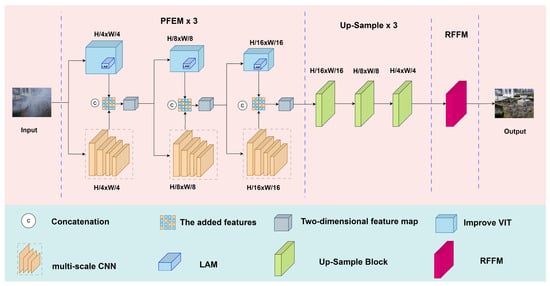
Figure 1.
Architecture of the proposed PID-Net for image dehazing.
The proposed architecture is composed of three core modules: (1) the Parallel Feature Extraction Module (PFEM), (2) the Lightweight Attention Module (LAM), and (3) the Redundant Feature Filtering Module (RFFM). The hazy input image is initially processed by the PFEM module, which concurrently extracts local and global features through dual pathways. The global feature branch employs the LAM module, a lightweight version of the ViT’s multi-head attention mechanism, while the local feature branch utilizes a multi-scale CNN. The extracted features are subsequently fused via channel-wise concatenation and propagated to the subsequent PFEM module. The fused output features from the final PFEM module undergo progressive refinement through a CNN decoder-based up-sampling module, followed by the RFFM module, ultimately reconstructing a high-quality restored image with enhanced structural and textural fidelity.
3.1. Parallel Feature Extraction Module (PFEM)
The PFEM, depicted in Figure 2, is the core of PID-Net, responsible for simultaneously extracting local and global features. It comprises two parallel branches: a multi-scale CNN branch for local feature extraction and a lightweight ViT branch for global feature extraction. In the CNN branch, the input first undergoes four multi-scale convolutional operations, respectively. The resulting feature maps are then concatenated along the channel dimension to generate a fused local feature map that encapsulates both spatial and channel-wise information. The final output of the ViT branch is the feature vector. To enable channel-wise concatenation with the CNN-derived feature map, this vector is processed by a dimensional alignment module, where the rearrange function reshapes it into a spatially structured feature map format. A convolutional layer is subsequently appended to refine the reshaped feature map, ensuring smoothness in both spatial and channel dimensions. Finally, the output feature maps from both the CNN and ViT branches are concatenated along the channel axis, forming the aggregated output of the PFEM module. The input of the model will gradually reduce the resolution of the feature map every time it passes through the PFEM module, and the sizes are H/4 × W/4, H/8 × W/8, and H/16 × W/16, respectively.
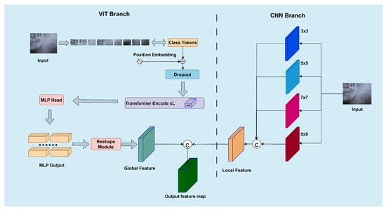
Figure 2.
Parallel Feature Extraction Module.
A multi-scale CNN employs a four-layer CNN with varying kernel sizes (3 × 3, 5 × 5, 7 × 7, and 9 × 9) to capture local features at multiple scales. The use of multi-scale kernels was inspired by the fact that haze affects image details at different scales. Larger convolutional kernels enable the extraction of wide-range contextual features, whereas smaller kernels focus on finer details like edges and textures. This multi-scale strategy ensures comprehensive local feature extraction, leading to better detail and texture restoration. The convolution operation in each layer can be represented by Equation (1) []:
In this context, Equation (1) utilizes a standard convolutional operation, following the typical form widely used in Convolutional Neural Networks. Here, the parameter x represents the input feature map, represents the convolution kernel with the size of , b represents the bias term for it, and represents the activation function acting on the convolution output. The local features extracted by the multi-scale CNN kernel network are represented as presented in Equation (2):
Here, represent convolutions of different kernel sizes, stack represents a concatenation operation that combines feature maps from different convolutional branches along the channel axis, and represents the output of the local feature map after channel-wise concatenation.
The global feature extraction branch utilizes a lightweight ViT to capture extensive receptive field information while maintaining parameter efficiency. To address the computational burden of a standard ViT, especially in high-resolution image processing, this paper proposes a Lightweight Attention Module, described in Section 3.2. During the initial stage, the raw image is uniformly segmented into discrete tiles of dimension L × L with no overlapping regions. Given an input image of H (height) × W (width), the image is split into HW/(L × L) smaller patches. These segmented patches undergo linear transformation to be embedded within a D-dimensional feature space. Subsequently, the Class Token is introduced to adaptively learn the spatial distribution characteristics of the non-uniform haze, enhancing dehazing performance in heterogeneous regions while maintaining global consistency in the color and illumination of the restored image. Additionally, spatial position information unique to the transformer network is incorporated. Once the image patches are embedded with spatial information, the resulting composite representations establish the essential token bank for subsequent attention operations, as presented in Equation (3) []:
Here, the complete token sequence comprises elements, where N corresponds to the number of image patches and the additional unit represents the class token, while D indicates the dimensionality of the embedded feature space. Additionally, the ViT autonomously acquires positional encoding parameters Epos through training, with the final input representation formed by the element-wise summation, and the final input sequence is represented as X + Epos of the patch embeddings and their spatial coordinates.
Additionally, the ViT uses the standard transformer encoder for the image patch sequence. The transformer encoder consists of four components: layer Normalization, multi-head attention mechanism, dropout, and MLP module. The layer Normalization layer is used to accelerate convergence and stabilize gradients. The multi-head attention mechanism extracts key information from the input by representing different spatial features. Dropout, implemented as drop path, improves training effectiveness, and the MLP module is used to process and output results. This setup enhances the generative performance of the transformer and stabilizes the training.
After extracting local features and global features, they are fused to form a new feature representation. First, the process applies pointwise convolution and sigmoidal normalization to global features to produce a weight map, as formulated in Equation (4). The weighted local features are subsequently concatenated with the global pathway outputs along the channel axis, which facilitates comprehensive feature integration across different receptive fields. By using the weights generated from the global features to modulate the local features, the fused features not only preserve local detail contours but also reflect global characteristics, significantly enhancing the dehazing performance of the model, as formulated in Equation (5).
Here, denotes the pointwise convolution operation, and the symbol ⊙ indicates element-level multiplication. The variables and , respectively, correspond to region features and holistic features, while is the final output.
3.2. Lightweight Attention Module (LAM)
The LAM, illustrated in Figure 3, is a modified multi-head attention mechanism designed to reduce computational cost while preserving performance. The key idea is to downsample the spatial resolution of the feature maps prior to attention computation and then compensate for the potential information loss using a CNN. Specifically, spatial down-sampling transforms input features from (C, H, W) to (C0, H/2, W/2) prior to query projection in the attention mechanism. However, this methodology may result in a loss of representational power for attention computation on low-resolution feature maps. To address the precision loss caused by this lightweight processing, this paper integrates a CNN network to restore the lost precision. This network includes a 3 × 3 depth convolution and a GeLU activation function, and it is applied to the Value part of the attention mechanism, which forms the foundation of the attention output. This enhancement improved the spatial information aggregation ability of the input features, thus strengthening representation, reducing training difficulty, and minimizing accuracy loss due to reduced computational costs.
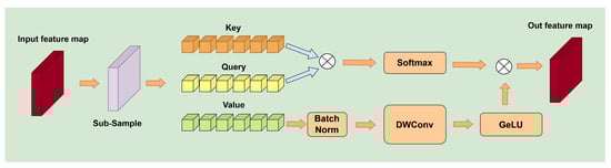
Figure 3.
Lightweight Attention Module.
The proposed lightweight attention mechanism can be formally defined by the following equation, where is a normalization function and is defined as presented in Equation (6) []:
where Q represents the Query matrix and denotes the transposed Key matrix. The parameter d, indicating the per-head channel dimensionality of both the Query and Key matrices, works in conjunction with trainable bias to modulate attention computations; is the final output. The definition of is provided in Equation (7):
where V represents the Value Matrix, denotes depthwise convolution, and represents Batch Norm for batch normalization.
3.3. Redundant Feature Filtering Module (RFFM)
The RFFM, shown in Figure 4, is designed to suppress redundant features, such as noise and residual haze, that may be introduced during the dehazing process.
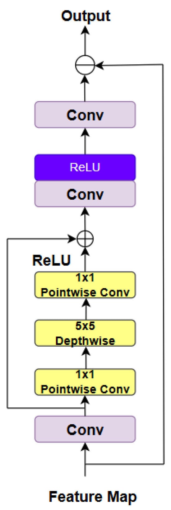
Figure 4.
Redundant Feature Filtering Module.
For the RFFM block, its input is derived from the outputs of the preceding up-sampling operations. Specifically, the RFFM processes feature maps generated through three PFEM-based down-sampling stages (integrating the CNN and ViT branches) and three subsequent up-sampling stages. These feature maps retain multi-scale and multi-semantic information but exhibit redundancy in representation. The primary function of the RFFM is to refine these feature maps by eliminating redundant patterns, utilizing a depthwise separable convolution network with residual learning and multi-layer convolutions. This enhances feature extraction through convolutional layers and residual learning, followed by multi-layer convolutions and local feature fusion to enrich feature representations. Ultimately, the feature representation is projected back to the initial representation space. After the mapping of the features is completed, the original input data are subtracted by a precise calculation method. The purpose of this subtraction operation is to effectively highlight those key differences.
The main calculation formula is as presented in Equation (8). represents pointwise convolution with a kernel size of 1 × 1, while represents depthwise convolution with a kernel size of 5 × 5. This module effectively integrates the image’s feature information, facilitating the transmission of information to deeper layers and enhancing the subtle features and texture information of the background image.
3.4. Loss Functions
This study adopts three distinct loss functions to regularize the parameter learning direction during network training: Smooth L1 Loss [], Perceptual Loss [], and Multi-Scale Structural Similarity (MS-SSIM) Loss []. The Smooth L1 Loss serves as the primary regularization term to minimize pixel-wise discrepancies between images, while the Perceptual Loss and MS-SSIM Loss are jointly applied to align the outputs with human visual perception characteristics.
Smooth L1 Loss: In image-dehazing tasks, preserving fine-grained details is critical for reconstructing high-fidelity, artifact-free results. Smooth L1 Loss function demonstrates superior performance in retaining structural details while mitigating distortion artifacts caused by overemphasis on minor pixel-level discrepancies, as compared to conventional Mean Squared Error (MSE) and L2 loss functions []. This advantage has been extensively validated across diverse image restoration benchmarks [], where Smooth L1 Loss achieves a balanced trade-off between robustness to outliers and sensitivity to subtle textures. The mathematical formulations of Smooth L1 Loss are defined in Equations (9) and (10):
Here, and represent the i-th pixel of the hazy and corresponding clear image, N is the total number of image pixels, and denotes the output image from the model.
Perceptual Loss: In image-restoration tasks, Perceptual Loss is widely used to measure the perceptual differences between two images and can capture more detailed information. This paper uses Perceptual Loss to obtain high-level perceptual information between dehazed and clear images to optimize network parameters. Perceptual Loss is computed using features extracted by a pretrained VGG16 [], as shown in Equation (11):
Here, x represents the hazy image, denotes the dehazed image output by the model, y is the original clear image, and represents the feature maps. The L2 loss is employed to measure the distance between them, where N indicates the number of features.
MS-SSIM Loss: In order to improve the visual effect, the third loss function uses MS-SSIM. This loss measures the similarity between two images by comparing the structural information of the image at different scales. Compared with the traditional pixel-level loss function, this loss can capture the structural information of the image, rather than relying solely on the comparison of pixel values, as shown in Formulas (12) and (13):
Here, O and G denote the windows centered and the i-th pixel in the images, respectively, and represent their corresponding means, and are the variances, is the covariance, and are constants, n indicates the number of scales, and corresponds to the associated weights.
The total loss function is defined as shown in Equation (14):
The weights () are utilized to balance the network’s loss function, facilitating the update and optimization of the network parameters through the total loss. Drawing from training experience, the values of , , and are assigned as 1, 0.01, and 0.5, respectively.
4. Experiments
For this section, this paper compared the proposed image-dehazing method with different dehazing algorithms on multiple datasets and confirmed its excellent performance. The experimental setup, dataset, evaluation criteria, and results were detailed, and ablation experiments were performed to evaluate the component contributions.
4.1. Experimental Setup
For the hardware setup, our experiments used an Nvidia GeForce RTX 3090 graphics card (Nvidia Corporation, Santa Clara, CA, USA). The algorithm was implemented with PyTorch version 1.13.1 and CUDA version 11.7 acceleration to enhance computational efficiency during both model training and testing. To accelerate convergence and adapt to model inputs, each image was randomly cropped to a size of 256 × 256. We employed the Adam optimizer with default parameters ( and ), setting the initial learning rate to 0.0001 and dynamically adjusting it using a cosine annealing scheduler []. To prevent overfitting and enhance training efficiency, an early stopping strategy was implemented, terminating the training automatically if the evaluation metric showed no improvement for 10 consecutive epochs. Complete hyperparameter configurations are provided in Table 1.

Table 1.
Experimental setup.
The Cosine Annealing algorithm [] is an optimization technique designed to dynamically adjust the learning rate during neural network training. The core principle involves utilizing the cosine function to modulate the learning rate, ensuring a smooth and gradual reduction over time, as opposed to the abrupt decay characteristic of linear strategies. Specifically, the learning rate transitions from an initial maximum value to a predefined minimum across training epochs. This smooth variation mitigates the risk of the model converging to local minima or experiencing oscillations during optimization. The learning rate for each epoch is computed according to Equation (15):
where denotes the current epoch index and represents the total number of training epochs. Finally, the model parameters are updated using the computed learning rate .
4.2. Datasets
In this study, in order to evaluate the performance of the proposed model more comprehensively, four datasets with different characteristics were carefully selected and used: RESIDE-6K-IN [], RESIDE-6K-OUT [], NH-HAZE [], and DENSE-HAZE []. These datasets were carefully chosen to evaluate the model’s efficacy across diverse dehazing scenarios.
- DENSE-HAZE: This dataset carefully collected and organized 55 pairs of real haze images and their corresponding smog-free images. The dehaze scene with uniform distribution of haze was simulated.
- NH-HAZE: This dataset comprised images depicting non-homogeneous atmospheric conditions, including 55 paired samples of haze scenes from the real world, corresponding to clear images of the ground. The hazy images were collected under the real hazy conditions created by the professional haze machine, and the haze distribution was uneven, offering the advantage of high fidelity in simulating real-world haze conditions.
- RESIDE-IN and RESIDE-OUT: The RESIDE-IN and RESIDE-OUT datasets were derived from the RESIDE-6K dataset [], which includes both synthetic and real-world images intended to simulate various weather conditions. This paper selected two scenes from this dataset, indoor and outdoor, which together had a total of 6000 image pairs.
4.3. Comparative Methods and Evaluation Metrics
To verify the effectiveness of the suggested approach, this paper contrasted it with seven mainstream dehazing algorithms—(D4 [], C2PNet [], EPDN [], GCANet [], SLP [], DEA-Net [], and TransDehaze [])—using synthetic and real-world datasets. For quantitative evaluation of image restoration quality, this paper used commonly employed metrics such as the Peak Signal-to-Noise Ratio (PSNR) and the Structural Similarity Index Measure (SSIM) to compare the performance of each algorithm.
4.4. Experimental Results
This study established a dual-index evaluation system utilizing PSNR and SSIM to conduct a comprehensive and objective assessment of multiple dehazing algorithms, including the proposed method. As shown in Table 2, compared with seven mainstream comparative methods, our approach achieved average improvements of 1.301 in PSNR and 0.014 in SSIM, demonstrating significant numerical advantages. The proposed method achieved optimal PSNR performance across both real-world and synthetic datasets. Regarding the SSIM metrics, while not attaining the highest value on the DENSE dataset, our method closely approached the maximum performance level observed in this benchmark.
Table 2.
Objective comparison results of different dehazing algorithms. The sign “-” indicates that the digit is unavailable, and bold typeface highlights the best performance.
In addition, the computational complexity of the competitive methods was quantitatively assessed using two main metrics: (1) the count of trainable parameters (Params), which reflects memory usage, and (2) the number of floating-point operations (FLOPs), indicating the theoretical computational cost. As shown in Table 2, models such as GCANet and D4 demonstrated a significant advantage in resource efficiency, but at the expense of reduced performance. The DEA-Net and TransDehaze models had relatively high FLOPs and parameter counts, meaning that while they pursued high performance, they also incurred a higher cost in terms of resource consumption. In contrast, our proposed model achieved the best results at a comparable cost. Future work will continue to explore further reductions in computational overhead while maintaining performance advantages.
Qualitative assessment of dehazing performance was conducted through subjective visual inspection, with the evaluation criteria emphasizing three key aspects: (a) degree of haze removal, (b) color consistency, and (c) detail preservation.
Results on real-world datasets. Initial algorithm evaluations were performed on two real-world datasets: DENSE-HAZE (uniform haze) and NH-HAZE (non-uniform haze). Visual results comparing haze removal and detail recovery are provided in Figure 5 and Figure 6:
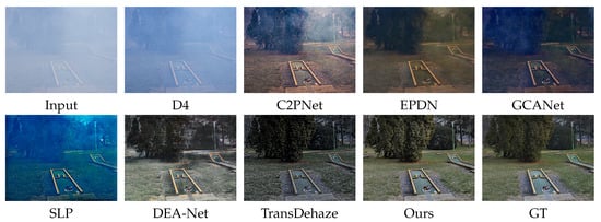
Figure 5.
Subjective visual quality comparison of different dehazing algorithms on DENSE-HAZE dataset.
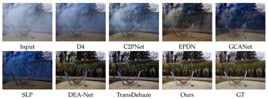
Figure 6.
Subjective visual quality comparison of different dehazing algorithms on NH-HAZE dataset.
As presented in Figure 5, our experimental results based on the DENSE-HAZE dataset show that the dehazing effects of D4 and C2PNet were mediocre, with residual haze to varying degrees. GCANet and SLP produced color distortion, and the excessively blue hue affected the natural appearance of the images. The EPDN method achieved relatively natural color restoration, with the overall tone being slightly cool. DEANet and TransDehaze exhibited excellent dehazing performance, but they still needed improvement, in terms of color saturation and detail sharpness.
As presented in Figure 6, our experiments on the more challenging NH-HAZE dataset revealed that the dehazing effects of the D4, C2PNet, and SLP methods were not obvious enough and that the tones were on the darker side. The EPDN and GCANet methods still had residual haze, and the color restoration needed to be optimized, resulting in mediocre overall performance. DEA-Net effectively removed the haze, making the scene structure clearly visible, but there was still a small amount of haze in some areas. TransDehaze achieved satisfactory dehazing results, but the details in the green vegetation areas were not clear enough.
Compared with the above methods, the proposed algorithm demonstrated obvious advantages in terms of the dehazing effect on the real-world datasets (DENSE-HAZE and NH-HAZE), while retaining sufficient image details, maintaining optimal color contrast, and achieving the highest visual similarity to the ground truth. These results align with the findings presented in Table 2. This advantage can be attributed to the strong feature extraction capability enabled by the dual-branch architecture.
Results on synthetic datasets. This paper tested different dehazing algorithms on the synthetic hazy datasets RESIDE-6K-OUT and RESIDE-6K-IN, with the dehazing results shown in Figure 7 and Figure 8:
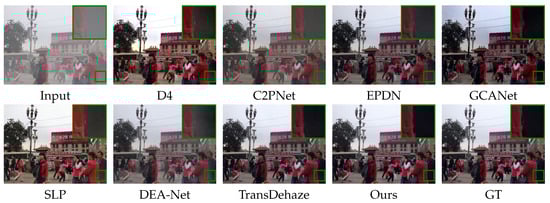
Figure 7.
Subjective visual quality comparison of different dehazing algorithms on RESIDE-OUT dataset.
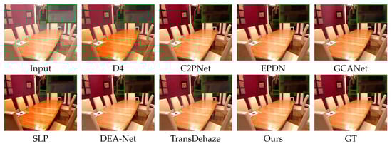
Figure 8.
Subjective visual quality comparison of different dehazing algorithms on RESIDE-IN dataset.
As presented in Figure 7, on the RESIDE-OUT dataset, on the whole, the D4 and SLP methods achieved better dehazing performance, but the color saturation was slightly too high. The clarity of the C2PNet and DEA-Net methods needs to be improved. The GCANet method had a slight color deviation in the sky area. From the local perspective (the green box selection part), it is evident that all the compared methods displayed varying levels of residual haze, artifacts, and undesirable blurring effects.
As presented in Figure 8, on the RESIDE-IN dataset, all the methods showed relatively good overall dehazing performance, but there was still room for improvement in dehazing integrity and color fidelity. Specifically, the D4 and SLP methods had slightly higher color saturation, resulting in a slight color deviation on the desktop surface; the tone reduction of the C2PNet and EPDN methods in the lower-left corner region was slightly insufficient. From the perspective of the local amplification area (the green box selection part), the dehazing effect of the D4, SLP, and TransDehaze methods had not been completely thorough, while the DEA-Net, EPDN, and GCANet methods still need to be further improved, in terms of detail clarity.
Through the comparisons on the synthetic datasets (RESIDE-OUT and RESIDE-IN), it can be found that the proposed method achieved remarkable results in haze removal. Specifically, its color reproduction, contrast, and brightness levels exhibited closer alignment with ground truth measurements compared to the other methods. These results align with the findings presented in Table 2. While the perceptual enhancements may appear subtle in certain scenarios, they nevertheless substantiated PID-Net’s consistent performance across diverse environmental conditions.
4.5. Ablation Study
In order to thoroughly evaluate the contribution of each module to the overall effect, this paper conducted an ablation study of the proposed PID-Net to demonstrate its effectiveness by disabling certain modules in the model. The ablation experiments were performed using the NH-HAZE dataset for training and testing, with the base model being the original ViT model. As presented in Table 3, the comparison results with the base model demonstrate that all the innovative modules significantly improved the model performance, thereby proving the effectiveness of our method.
Table 3.
Objective comparison results of ablation experiment. The bold typeface highlights the best performance.
- Base-LAM: After replacing the standard multi-head attention mechanism with LAM, the number of parameters decreased from 30.7 M to 28.6 M and FLOPs were reduced from 24.35 G to 18.71 G, while PSNR and SSIM improved from 12.527 and 0.462 to 13.576 and 0.509, respectively. This demonstrates that the LAM module not only reduces the computational cost but also improves the performance of the model through the CNN compensation mechanism, realizing the double optimization of efficiency and accuracy.
- Base+Multi-CNN: Incorporating a multi-scale convolutional network into the Base model led to a significant improvement in the PSNR and SSIM, increasing from 13.576 and 0.509 to 17.609 and 0.633, respectively. This validates the effectiveness of a multi-scale CNN in capturing local haze features and enhancing detail restoration. The parallel processing of local and global features significantly improved dehazing performance, albeit with a corresponding increase in parameters and FLOPs.
- Base+Multi-CNN+RFFM: With the addition of the RFFM, the PSNR and SSIM further increased to 18.625 and 0.675, respectively. This indicates that the RFFM effectively filters out redundant features, generating cleaner dehazed images. By suppressing noise and haze-related information, this module enables the model to focus on learning more discriminative dehazing features.
- Ours: The best performance was achieved by integrating LAM, Multi-CNN, and RFFM into the Base model, with the PSNR and SSIM reaching 20.358 and 0.745, respectively. Analysis of the model’s parameters revealed that, despite several enhancements, the number of parameters had only increased slightly and the FLOPs had decreased instead compared with the Base model. The reason was that the down-sampling operation reduced the size of the features in the middle layer, thereby reducing the computational load of the model. This result further proves the efficiency provided by incorporating LAM.
As presented in Figure 9, the visual comparisons in the ablation studies clearly demonstrate that the proposed model exhibited superior performance under the specified experimental conditions and environments. The resulting images exhibit improved dehazing, color restoration, and detail representation, closely approximating real images and confirming the effectiveness of the introduced modules.
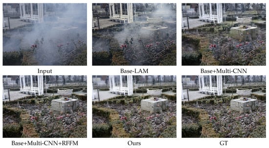
Figure 9.
Visual comparison results of ablation experiments.
5. Conclusions
This study introduces PID-Net, a novel Parallel Image-Dehazing Network designed to address key challenges in hazy scene processing, including effective haze removal, detail preservation, and accurate color restoration. PID-Net integrates the parallel architecture of a multi-scale CNN and a ViT, enabling effective extraction of rich local details and global semantic information. A lightweight attention mechanism and a CNN compensation module within the ViT branch reduce computational overhead while maintaining performance. Furthermore, a Redundant Feature Filtering Module effectively suppresses noise and haze-related artifacts, resulting in cleaner dehazed images. Comprehensive experiments on four standard datasets validated PID-Net’s superior performance, demonstrating notable gains in PSNR/SSIM scores and perceptual quality.
In addition, the proposed method has potential applicability in other key areas, such as optical image encryption [,], where the image quality is generally affected (hazy artifacts) by the decryption process using optical transform, as well as biomedical imaging approaches such as optical coherence tomography [], where the generated image has been affected (hazy artifacts) by optical aberration and noise. Future work will focus on enhancing the practicality and applicability of PID-Net. The current network, due to its size and parameter count, presents deployment challenges, particularly on lower-end devices. Model simplification and parameter reduction are, therefore, crucial. Additionally, training with diverse datasets is necessary to improve generalization ability. These improvements will reduce application costs, enhance versatility, and are of significant importance for real-world deployment.
Author Contributions
Conceptualization, W.L.; methodology, Y.Z. and W.L.; software, Y.Z. and D.Z.; validation, Y.Z. and W.L.; writing—original draft preparation, Y.Z. and W.L.; writing—review and editing, Y.Z., W.L., D.Z. and Y.Q. All authors have read and agreed to the published version of the manuscript.
Funding
This work received partial support from the Key Scientific and Technological Project of Henan Province, under Grants 252102210161 and 232102211059, and also from the Nanyang Normal University Foundation of China under Grant 2024PY011.
Data Availability Statement
The datasets used in this study are all publicly available benchmark datasets. The DENSE-HAZE dataset comes from the paper “Dense-haze: A benchmark for image dehazing with dense-haze and haze-free images” [], the NH-HAZE dataset is from “NH-HAZE: An image dehazing benchmark with non-homogeneous hazy and haze-free images” [], and the RESIDE-6K dataset originates from “Benchmarking single-image dehazing and beyond” [].
Conflicts of Interest
The authors declare no conflicts of interest.
References
- Guo, Q.; Feng, X.; Xue, P.; Sun, S.; Li, X. Dual-domain multi-scale feature extraction for image dehazing. Multimed. Syst. 2025, 31, 1–15. [Google Scholar] [CrossRef]
- He, K.; Sun, J.; Tang, X. Single image haze removal using dark channel prior. IEEE Trans. Pattern Anal. Mach. Intell. 2010, 33, 2341–2353. [Google Scholar] [PubMed]
- Zhu, Q.; Mai, J.; Shao, L. A fast single image haze removal algorithm using color attenuation prior. IEEE Trans. Image Process. 2015, 24, 3522–3533. [Google Scholar] [PubMed]
- Zhou, Y.; Chen, Z.; Li, P.; Song, H.; Chen, C.P.; Sheng, B. FSAD-Net: Feedback spatial attention dehazing network. IEEE Trans. Neural Netw. Learn. Syst. 2022, 34, 7719–7733. [Google Scholar] [CrossRef]
- Zhang, D.; Wang, Y.; Meng, L.; Yan, J.; Qin, C. Adaptive critic design for safety-optimal FTC of unknown nonlinear systems with asymmetric constrained-input. ISA Trans. 2024, 155, 309–318. [Google Scholar] [CrossRef]
- Zhao, X.; Xu, F.; Liu, Z. TransDehaze: Transformer-enhanced texture attention for end-to-end single image dehaze. Vis. Comput. 2024, 41, 1621–1635. [Google Scholar] [CrossRef]
- Chen, D.; He, M.; Fan, Q.; Liao, J.; Zhang, L.; Hou, D.; Yuan, L.; Hua, G. Gated context aggregation network for image dehazing and deraining. In Proceedings of the 2019 IEEE Winter Conference on Applications of Computer Vision (WACV), Waikoloa Village, HI, USA, 7–11 January 2019; pp. 1375–1383. [Google Scholar]
- Zhang, S.; He, F. DRCDN: Learning deep residual convolutional dehazing networks. Vis. Comput. 2020, 36, 1797–1808. [Google Scholar] [CrossRef]
- Chen, Z.; He, Z.; Lu, Z.M. DEA-Net: Single image dehazing based on detail-enhanced convolution and content-guided attention. IEEE Trans. Image Process. 2024, 33, 1002–1015. [Google Scholar] [CrossRef]
- Song, Y.; He, Z.; Qian, H.; Du, X. Vision transformers for single image dehazing. IEEE Trans. Image Process. 2023, 32, 1927–1941. [Google Scholar] [CrossRef]
- Liu, Z.; Lin, Y.; Cao, Y.; Hu, H.; Wei, Y.; Zhang, Z.; Lin, S.; Guo, B. Swin transformer: Hierarchical vision transformer using shifted windows. In Proceedings of the IEEE/CVF International Conference on Computer Vision, Montreal, BC, Canada, 11–17 October 2021; pp. 10012–10022. [Google Scholar]
- Guo, C.L.; Yan, Q.; Anwar, S.; Cong, R.; Ren, W.; Li, C. Image dehazing transformer with transmission-aware 3D position embedding. In Proceedings of the IEEE/CVF Conference on Computer Vision and Pattern Recognition, New Orleans, LA, USA, 18–24 June 2022; pp. 5812–5820. [Google Scholar]
- Ling, P.; Chen, H.; Tan, X.; Jin, Y.; Chen, E. Single image dehazing using saturation line prior. IEEE Trans. Image Process. 2023, 32, 3238–3253. [Google Scholar] [CrossRef]
- Cui, Z.; Wang, N.; Su, Y.; Zhang, W.; Lan, Y.; Li, A. ECANet: Enhanced context aggregation network for single image dehazing. Signal Image Video Process. 2023, 17, 471–479. [Google Scholar] [CrossRef]
- Zhang, D.; Hao, X.; Wang, D.; Qin, C.; Zhao, B.; Liang, L.; Liu, W. An efficient lightweight convolutional neural network for industrial surface defect detection. Artif. Intell. Rev. 2023, 56, 10651–10677. [Google Scholar] [CrossRef]
- Qu, Y.; Chen, Y.; Huang, J.; Xie, Y. Enhanced pix2pix dehazing network. In Proceedings of the IEEE/CVF Conference on Computer Vision and Pattern Recognition, Long Beach, CA, USA, 15–20 June 2019; pp. 8160–8168. [Google Scholar]
- Luo, P.; Xiao, G.; Gao, X.; Wu, S. LKD-Net: Large kernel convolution network for single image dehazing. In Proceedings of the 2023 IEEE International Conference on Multimedia and Expo (ICME), Brisbane, Australia, 10–14 July 2023; pp. 1601–1606. [Google Scholar]
- Yi, W.; Dong, L.; Liu, M.; Hui, M.; Kong, L.; Zhao, Y. SID-Net: Single image dehazing network using adversarial and contrastive learning. Multimed. Tools Appl. 2024, 83, 71619–71638. [Google Scholar] [CrossRef]
- Gao, G.; Cao, J.; Bao, C.; Hao, Q.; Ma, A.; Li, G. A novel transformer-based attention network for image dehazing. Sensors 2022, 22, 3428. [Google Scholar] [CrossRef]
- Yang, Y.; Zhang, H.; Wu, X.; Liang, X. MSTFDN: Multi-scale transformer fusion dehazing network. Appl. Intell. 2023, 53, 5951–5962. [Google Scholar] [CrossRef]
- Song, T.; Fan, S.; Li, P.; Jin, J.; Jin, G.; Fan, L. Learning an effective transformer for remote sensing satellite image dehazing. IEEE Geosci. Remote Sens. Lett. 2023, 20, 1–5. [Google Scholar] [CrossRef]
- Qiu, Y.; Zhang, K.; Wang, C.; Luo, W.; Li, H.; Jin, Z. Mb-taylorformer: Multi-branch efficient transformer expanded by taylor formula for image dehazing. In Proceedings of the IEEE/CVF International Conference on Computer Vision, Paris, France, 1–6 October 2023; pp. 12802–12813. [Google Scholar]
- Wang, Y.; Yan, X.; Wang, F.L.; Xie, H.; Yang, W.; Zhang, X.P.; Qin, J.; Wei, M. UCL-Dehaze: Toward real-world image dehazing via unsupervised contrastive learning. IEEE Trans. Image Process. 2024, 33, 1361–1374. [Google Scholar] [CrossRef]
- Xu, J.; Chen, Z.X.; Luo, H.; Lu, Z.M. An efficient dehazing algorithm based on the fusion of transformer and convolutional neural network. Sensors 2022, 23, 43. [Google Scholar] [CrossRef]
- Szegedy, C.; Liu, W.; Jia, Y.; Sermanet, P.; Reed, S.; Anguelov, D.; Erhan, D.; Vanhoucke, V.; Rabinovich, A. Going deeper with convolutions. In Proceedings of the IEEE Conference on Computer Vision and Pattern Recognition, Boston, MA, USA, 7–12 June 2015; pp. 1–9. [Google Scholar]
- Dosovitskiy, A.; Beyer, L.; Kolesnikov, A.; Weissenborn, D.; Zhai, X.; Unterthiner, T.; Dehghani, M.; Minderer, M.; Heigold, G.; Gelly, S.; et al. An image is worth 16 × 16 words: Transformers for image recognition at scale. arXiv 2020, arXiv:2010.11929. [Google Scholar]
- Zhang, T.; Li, L.; Zhou, Y.; Liu, W.; Qian, C.; Hwang, J.N.; Ji, X. Cas-vit: Convolutional additive self-attention vision transformers for efficient mobile applications. arXiv 2024, arXiv:2408.03703. [Google Scholar]
- Girshick, R. Fast r-cnn. In Proceedings of the IEEE International Conference on Computer Vision, Santiago, Chile, 7–13 December 2015; pp. 1440–1448. [Google Scholar]
- Johnson, J.; Alahi, A.; Fei-Fei, L. Perceptual losses for real-time style transfer and super-resolution. In Proceedings of the Computer Vision–ECCV 2016: 14th European Conference, Amsterdam, The Netherlands, 11–14 October 2016; Proceedings, Part II 14. Springer: Berlin/Heidelberg, Germany, 2016; pp. 694–711. [Google Scholar]
- Wang, Z.; Bovik, A.C.; Sheikh, H.R.; Simoncelli, E.P. Image quality assessment: From error visibility to structural similarity. IEEE Trans. Image Process. 2004, 13, 600–612. [Google Scholar] [CrossRef] [PubMed]
- Yu, Y.; Liu, H.; Fu, M.; Chen, J.; Wang, X.; Wang, K. A two-branch neural network for non-homogeneous dehazing via ensemble learning. In Proceedings of the IEEE/CVF Conference on Computer Vision and Pattern Recognition, Nashville, TN, USA, 20–25 June 2021; pp. 193–202. [Google Scholar]
- Zhao, H.; Gallo, O.; Frosio, I.; Kautz, J. Loss functions for image restoration with neural networks. IEEE Trans. Comput. Imaging 2016, 3, 47–57. [Google Scholar] [CrossRef]
- Simonyan, K.; Zisserman, A. Very deep convolutional networks for large-scale image recognition. arXiv 2014, arXiv:1409.1556. [Google Scholar]
- Li, B.; Ren, W.; Fu, D.; Tao, D.; Feng, D.; Zeng, W.; Wang, Z. Benchmarking single-image dehazing and beyond. IEEE Trans. Image Process. 2018, 28, 492–505. [Google Scholar] [CrossRef]
- Ancuti, C.O.; Ancuti, C.; Timofte, R. NH-HAZE: An image dehazing benchmark with non-homogeneous hazy and haze-free images. In Proceedings of the IEEE/CVF Conference on Computer Vision and Pattern Recognition Workshops, Seattle, WA, USA, 14–19 June 2020; pp. 444–445. [Google Scholar]
- Ancuti, C.O.; Ancuti, C.; Sbert, M.; Timofte, R. Dense-haze: A benchmark for image dehazing with dense-haze and haze-free images. In Proceedings of the 2019 IEEE International Conference on Image Processing (ICIP), Taipei, Taiwan, 22–25 September 2019; pp. 1014–1018. [Google Scholar]
- Yang, Y.; Wang, C.; Liu, R.; Zhang, L.; Guo, X.; Tao, D. Self-augmented unpaired image dehazing via density and depth decomposition. In Proceedings of the IEEE/CVF Conference on Computer Vision and Pattern Recognition, New Orleans, LA, USA, 18–22 June 2022; pp. 2037–2046. [Google Scholar]
- Zheng, Y.; Zhan, J.; He, S.; Dong, J.; Du, Y. Curricular contrastive regularization for physics-aware single image dehazing. In Proceedings of the IEEE/CVF Conference on Computer Vision and Pattern Recognition, Vancouver, BC, Canada, 17–24 June 2023; pp. 5785–5794. [Google Scholar]
- Kumar, M.R.; Linslal, C.; Pillai, V.M.; Krishna, S.S. Color image encryption and decryption based on jigsaw transform employed at the input plane of a double random phase encoding system. In Proceedings of the International Congress on Ultra Modern Telecommunications and Control Systems, Moscow, Russia, 18–20 October 2010; pp. 860–862. [Google Scholar]
- Singh, P.; Agrawal, B.; Chaurasiya, R.K.; Acharya, B. Low-area and high-speed hardware architectures of KLEIN lightweight block cipher for image encryption. J. Electron. Imaging 2023, 32, 013012. [Google Scholar] [CrossRef]
- Kolokoltsev, O.; Gómez-Arista, I.; Treviño-Palacios, C.G.; Qureshi, N.; Mejia-Uriarte, E.V. Swept source OCT beyond the coherence length limit. IEEE J. Sel. Top. Quantum Electron. 2016, 22, 222–227. [Google Scholar] [CrossRef]
Disclaimer/Publisher’s Note: The statements, opinions and data contained in all publications are solely those of the individual author(s) and contributor(s) and not of MDPI and/or the editor(s). MDPI and/or the editor(s) disclaim responsibility for any injury to people or property resulting from any ideas, methods, instructions or products referred to in the content. |
© 2025 by the authors. Licensee MDPI, Basel, Switzerland. This article is an open access article distributed under the terms and conditions of the Creative Commons Attribution (CC BY) license (https://creativecommons.org/licenses/by/4.0/).