Unmanned Aerial Vehicle Path Planning Using Acceleration-Based Potential Field Methods

Abstract

Online path planning for UAVs that are following a moving target is a critical component in applications that demand a soft landing over the target. In highly dynamic situations with accelerating targets, the classical potential field (PF) method, which considers only the relative positions and/or velocities, cannot provide precision tracking and landing. Therefore, this work presents an improved acceleration-based potential field (ABPF) path planning method. This approach incorporates the relative accelerations of the UAV and the target in constructing an attractive field. By controlling the acceleration, the ABPF produces smoother trajectories and avoids sudden changes in the UAV’s motion. The proposed approach was implemented in different simulated scenarios with variable acceleration paths (i.e., circular, infinite, and helical). The simulation demonstrated the superiority of the proposed approach over the traditional PF. Moreover, similar path scenarios were experimentally evaluated using a quadrotor UAV in an indoor Vicon positioning system. To provide reliable estimations of the acceleration for the suggested method, a non-linear complementary filter was used to fuse information from the drone’s accelerometer and the Vicon system. The improved PF method was compared to the traditional PF method for each scenario. The results demonstrated a 50% improvement in the position, velocity, and acceleration accuracy across all scenarios. Furthermore, the ABPF responded faster to merging with the target path, with rising times of 1.5, 1.6, and 1.3 s for the circular, infinite, and helical trajectories, respectively.

1. Introduction

Path planning is an essential component of cooperative missions with UAV formations completing complex and variable tasks, such as search and rescue, surveillance, monitoring, and inspections [1]. Path planning algorithms can be classified into two types—global and local [2]. Global path planning algorithms are presented as static programming algorithms that use map information to generate an optimal trajectory from the starting point to the target point. On the other hand, local path planning algorithms are dynamic algorithms that consider the current pose information in real time, as provided by onboard sensors, and calculate the optimal trajectory between the starting and ending points.

Among other dynamic path planning algorithms, the dynamic window approach (DWA), the mathematical optimization algorithm (MOA), model predictive control (MPC), and the potential field (PF) are widely used in robot dynamic path planning. The DWA produces path candidates by developing the velocity space that can be formed by the present robot velocities [3]. The DWA then chooses the best path from these path candidates, assuming static obstacles. In [4], this method was developed to include dynamic obstacles, utilizing neural networks to estimate the weights of the DWA, which were subsequently employed for safe local navigation. In order to consider static and dynamic obstacles and guarantee path candidates at variable velocities, the DWA was proposed with virtual manipulators (DWVs) in [5]. However, DWA-based approaches are not ideal for environments with many dynamic obstacles. On the other hand, the mathematical optimization algorithm (MOA) relies on the existing robot trajectory planning model to solve the optimal control problem. The MOA transforms the optimal control problem into an easily solvable model by employing several mathematical techniques, such as non-linear optimization, mixed integer linear programming (MILP), or dynamic programming (DP) [6,7,8].

Model predictive control (MPC) is used to construct a cost function over a fixed time interval in the future in order to determine the appropriate control sequence based on the robot’s predicted future behaviors. To ensure system stability, the cost function can be modeled as a Lyapunov function by including a terminal cost [9,10]. The tracking problem with obstacles remains one of the most difficult tasks. As a result, the potential field (PF) approach has been used to find a collision-free path through an obstacle-filled environment [11,12]. Despite advances in these techniques, the MOA and MPC remain computationally demanding and necessitate a precise understanding of the robot’s dynamics. Furthermore, the real-time implementation of these algorithms may be difficult for fast robots or extremely dynamic settings. Therefore, the PF is a commonly used method due to advantages such as its quick response time, low calculation requirements, and higher real-time precision [13]. Although the traditional PF method introduces the local minima problem, which traps an object before it reaches its destination, many researchers have been able to solve this problem, e.g., by using virtual obstacle or virtual target concepts [14,15] or by implementing a fuzzy system [16].

According to the concept of a potential field, a robot moves under the influence of a virtual attractive force that is required to pull it to a target, as well as simultaneous repulsive forces generated to avoid obstacles. These forces are determined by the robot’s relative position and velocity with respect to the target, as well as with respect to the obstacles encountered [16,17,18]. Traditionally, the attractive potential of a robot is determined by its relative position in relation to a fixed- or constant-velocity moving point in space [19]. However, when a target moves at various velocities, the position-based potential function is no longer appropriate. As a result, researchers have discovered that accounting for both the robot’s and target’s velocities is beneficial when designing a potential field [20,21].

Providing online path planning for UAVs during autonomous missions to precisely track a moving target in a highly dynamic environment is critical [22]. In many applications, the UAV must land precisely over a moving target to recharge during persistent flights [23]. Therefore, many studies have focused on upgrading the classic potential field method for UAV path planning. For example, a few attempts have been made to enhance the repulsive field, allowing for smoother obstacle avoidance [24,25], whereas others have improved the attractive field within the method for better target reachability [26]. Other techniques have addressed both the attractive and repulsive forces using the fuzzy-based method [16] or the Artificial Neural Network method [27]. However, all of the researchers in the literature have developed enhanced algorithms for the traditional potential field model, which only considers the position and velocity gradients. To this end, this paper presents an improved attractive field force by increasing the degrees of freedom by considering the acceleration differential between the target and the UAV.

The authors of [28] used the increased attractive force gain coefficient approach with increasing gradient in order to improve the performance of the attractive field in the PF. This strategy prevents oscillations and ensures that the UAV reaches the target. In a similar technique, the attractive force was enhanced by incorporating a damping force to prevent oscillations near the target [29,30]. In another study, a UAV path planning technique was proposed to offer a consistent and continuous coverage path over a ground robot in a windy environment. This method presented a novel modified attractive force to improve the sensitivity of a UAV to wind speed and direction [26]. Despite the efforts of researchers to enhance the attractive force in potential fields, they could not achieve precision in tracking an accelerating target for soft landing.

The acceleration of direction-turning drones was taken into consideration in waypoint-based path planning using the potential field method, as described in [31]. The study demonstrated the need to consider the acceleration of the drone at waypoints in time-critical applications, as ignoring acceleration leads to an unreasonably short flight. In [32], the relative acceleration term is considered for an attractive potential function in dynamic environments. This study created a two-dimensional function of relative acceleration, velocity, and position between the ground robot and the target. However, this work solely used simulations to examine the acceleration-based potential field functions. An exponential attractive function was adopted in [22], to provide different gradients for its force. Using this technique, the attractive force changes rapidly as the UAV approaches the target. It allowed the UAV to swiftly and effectively track the movement of a ground robot with varying velocity.

In soft-landing applications, the velocity and acceleration of the UAV must be equal to those of the target. As previously stated, the typical potential field function only considers the relative positions between the UAV and the target for the attractive potential force, which may result in jerky motion and rushed turns for the UAV. For this purpose, this study focuses on strengthening the attractive potential field model by incorporating the acceleration term in addition to velocity and position information. In this approach, the attractive force is expected to be more responsive, as it accounts for dynamic constraints and smoother motion. To help readers comprehend the contribution of this study, Table 1 summarizes the merits of earlier works in the literature and compares them to the suggested approach. To solve the motion-planning problem in dynamic environments with accelerating targets, we must assume the following:

Table 1. Comparison of the proposed method to various local path planning methods, including traditional PF.

Feature	DWA	MOA	MPC	PF	Acceleration Based-PF (Proposed)
Real-time Performance	High	Moderate to Low	Moderate to Low	High	High
Computational Load	Low	High	High	Low	Low
Handling Dynamic Obstacles	Moderate	No	Depending on the model accuracy	Moderate	Not investigated
Target Tracking Accuracy	Moderate	Moderate to Low	High (depending on the model and solver)	Low to Moderate	High
Landing Accuracy	Moderate	Moderate	Low to Moderate (depending on the model and solver)	Low to Moderate	High
Optimality	Heuristic (local)	Optimal (requiring careful tuning)	Optimal (requiring significant tuning)	Heuristic (local)	Heuristic (local)
Complexity	Low	High	High	Low	Low

(1)

Assumption 1. The shape, positions, velocities, and accelerations of the UAV are known.

(2)

Assumption 2. The position A_tar, velocity B_tar, and the acceleration C_tar of the target are known with |C_tar| < C_max.

The repulsive force will not be covered in this study. Acceleration-based improvements for repulsive force may be discussed in subsequent work in the future.

Following the introduction, the rest of this paper is organized as follows: Section 2 provides a full derivation of the suggested attractive potential field model. Section 3 proposes a motion planning strategy. Section 4 provides a detailed discussion of the supporting simulation. This work was evaluated experimentally under several settings, as described in Section 5. The conclusions and future research are presented in Section 6.

2. Acceleration-Based Attractive Potential Force

According to current approaches, the attractive potential force is determined solely by the relative velocity and position between the UAV and the target. In this study, the attractive potential force is defined by considering the relative position, velocity, and acceleration between the UAV and the target. The following equation defines the new attractive potential $V_{att}$:

$$V_{att}={\delta }_a{\parallel A_{tar}\left(t\right)-A_{UAV}\left(t\right)\parallel }^i+{\delta }_b{\parallel B_{tar}\left(t\right)-B_{UAV}\left(t\right)\parallel }^j+{\delta }_c{\parallel C_{tar}\left(t\right)-C_{UAV}\left(t\right)\parallel }^k$$

(1)

where $A_{tar}\left(t\right)$ and $A_{UAV}\left(t\right)$ represent the position of the target and UAV at a given instant t. The velocities of the target and UAV are represented by $B_{tar}\left(t\right)$ and $B_{UAV}\left(t\right)$ at a given instant t. The accelerations of the target and UAV are given by $C_{tar}\left(t\right)$ and $C_{UAV}\left(t\right)$ at a given instant t. The magnitude of the distance between the target and the UAV is denoted by $‖A_{tar}\left(t\right)-A_{UAV}\left(t\right)‖$. The magnitude of the relative velocity between the target and the UAV is indicated by $‖B_{tar}\left(t\right)-B_{UAV}\left(t\right)‖$, and $‖C_{tar}\left(t\right)-C_{UAV}\left(t\right)‖$ is the magnitude of the relative acceleration between the target and the UAV. ${\delta }_a$, ${\delta }_b$, and ${\delta }_c$ are positive parameters, while $i$, $j$, and $k$ are exponents.

To find the attractive force, the negative gradient of the attractive potentials is given by the following equation:

$$F_{att}\left(A,B,C\right)=-{\nabla }_A{V}_{att}\left(A,B,C\right)-{\nabla }_B{V}_{att}\left(A,B,C\right)-{\nabla }_C{V}_{att}\left(A,B,C\right)$$

(2)

where

$$F_{att1}=-{\nabla }_A{V}_{att}\left(A,B,C\right)=-{\displaystyle \frac{\mathsf{\partial }{V}_{att}\left(A,B,C\right)}{\mathsf{\partial }A}}$$

(3)

$${ F}_{att2}=-{\nabla }_B{V}_{att}\left(A,B,C\right)=-{\displaystyle \frac{\mathsf{\partial }{V}_{att}\left(A,B,C\right)}{\mathsf{\partial }B}}$$

(4)

$$F_{att3}=-{\nabla }_C{V}_{att}\left(A,B,C\right)=-{\displaystyle \frac{\mathsf{\partial }{V}_{att}\left(A,B,C\right)}{\mathsf{\partial }C}}$$

(5)

Regarding $i,j$, and $k$, as well as the differentiation of $V_{att}\left(A,B,C\right)$, we notice that $V_{att}\left(A,B,C\right)$ is not differentiable when $A_{tar}\left(t\right)=A_{UAV}\left(t\right)$ for $0<i\le 1$. Furthermore, this is not differentiable when $B_{tar}\left(t\right)=B_{UAV}\left(t\right)$ for $0<j\le 1$, or when $C_{tar}\left(t\right)=C_{UAV}\left(t\right)$ for $0<k\le 1$. In soft-landing applications, the UAV must reach the target with the same velocity and acceleration, which means that $A_{tar}\left(t\right)=A_{UAV}\left(t\right)$, $B_{tar}\left(t\right)=B_{UAV}\left(t\right)$, and $C_{tar}\left(t\right)=C_{UAV}\left(t\right)$. Therefore, for this purpose, the parameters are chosen such that $i,j$, and $k>1$.

In hard-landing applications, the UAV must reach the target with $B_{tar}\left(t\right)\ne B_{UAV}\left(t\right)$ and $C_{tar}\left(t\right)\ne C_{UAV}\left(t\right)$. In this case, only $i>1$ is selected.

Thus, the attractive force terms are defined as follows:

$$F_{att1}=i{\delta }_a{\parallel A_{tar}\left(t\right)-A_{UAV}\left(t\right)\parallel }^{i-1}{a}_{RT}$$

(6)

$$F_{att2}=j{\delta }_b{\parallel B_{tar}\left(t\right)-B_{UAV}\left(t\right)\parallel }^{j-1}{b}_{RT}$$

(7)

$$F_{att3}=k{\delta }_c{\parallel C_{tar}\left(t\right)-C_{UAV}\left(t\right)\parallel }^{k-1}{c}_{RT}$$

(8)

where $a_{RT}$ indicates the unit vector directed from the UAV to the target. $b_{RT}$ is the unit vector that directs the relative velocity vector from the target with respect to the UAV. $c_{RT}$ is the unit vector that directs the relative acceleration vector from the target with respect to the UAV. Figure 1 shows the relationship between the three attractive forces and the relative position, velocity, and acceleration vectors between the target and the UAV.

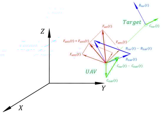
Figure 1. The three attractive forces and the relative position, velocity, and acceleration vectors between the target and the UAV.

3. Attractive Motion Planning Strategy for Unmanned Arial Vehicles

Newton’s second law states that the forces are equal to mass times acceleration, as follows:

$$F_{UAV}=m{C}_{UAV}$$

(9)

where $F_{UAV}$ is the desired force to be applied to the UAV in order to reach the target. The proposed attractive potential function includes six parameters—${\delta }_a,{\delta }_b, {\delta }_c, i,j,$ and $k$. Let us consider $i=j=k=2.$ The selection of these integers provides the best system performance, as explained in Section 4. Accordingly, the attractive force can be rewritten as follows:

$$F_{att}=2{\delta }_a\parallel A_{tar}\left(t\right)-A_{UAV}\left(t\right)\parallel +2{\delta }_b\parallel B_{tar}\left(t\right)-B_{UAV}\left(t\right)\parallel +2{\delta }_c\parallel C_{tar}\left(t\right)-C_{UAV}\left(t\right)\parallel$$

(10)

Let us apply the following force to the UAV:

$$F_{UAV}=m_{UAV}{C}_{tar}+F_{att }$$

(11)

Combining Equations (9)–(11) and setting $m_{UAV}=1$, we obtain the following equation:

$$C_{UAV}\left(t\right)=C_{tar}\left(t\right)+2{\delta }_a\parallel A_{tar}\left(t\right)-A_{UAV}\left(t\right)\parallel +2{\delta }_b\parallel B_{tar}\left(t\right)-B_{UAV}\left(t\right)+2{\delta }_c‖C_{tar}\left(t\right)-C_{UAV}\left(t\right)‖$$

(12)

Taking common factors and combining terms, we obtain:

$$\left(1+2{\delta }_c\right)\parallel C_{tar}\left(t\right)-C_{UAV}\left(t\right)\parallel +2{\delta }_b\parallel B_{tar}\left(t\right)-B_{UAV}\left(t\right)\parallel +2{\delta }_a\parallel A_{tar}\left(t\right)-A_{UAV}=0$$

(13)

It is known that the relative position between the UAV and the target is the error $e\left(t\right).$

So, rewriting Equation (13) gives the following equation:

$$\ddot{e}\left(t\right)+{\displaystyle \frac{2{\delta }_b}{\left(1+2{\delta }_c\right)}}\dot{e}\left(t\right)+{\displaystyle \frac{2{\delta }_a}{\left(1+2{\delta }_c\right)}}e\left(t\right)=0$$

(14)

Now, by comparing Equation (14) with the characteristic equation of a second-order system, we obtain the following:

$$s^2+2\zeta {\omega }_{n}s+{\omega }_n^2=0$$

(15)

Keep in mind that $\zeta$ is the damping ratio and ${\omega }_n$ is the natural frequency of the system. Because ${\delta }_a,{\delta }_b$, and ${\delta }_c$ are positive parameters, the system is considered stable.

Now,

$${\omega }_n^2={\displaystyle \frac{2{\delta }_a}{\left(1+2{\delta }_c\right)}} \mathrm{then} {\omega }_n=\sqrt{{\displaystyle \frac{2{\delta }_a}{\left(1+2{\delta }_c\right)}}}$$

(16)

and

$$2\zeta {\omega }_n={\displaystyle \frac{2{\delta }_b}{\left(1+2{\delta }_c\right)}}$$

(17)

By substituting (16) into (17) and substituting $\zeta =1$ to obtain a critically damped system, we obtain the following equation:

$${\displaystyle \frac{{\delta }_b^2}{{2\delta }_a}}-1=2{\delta }_c$$

(18)

Keep in mind that ${\delta }_a,{\delta }_b$, and ${\delta }_c$ must be positive values to guarantee stability, such that ${\delta }_a>0$, ${\delta }_b>0$, and ${\delta }_c>0$.

$${\delta }_c>0 \mathrm{then} 2{\delta }_c>0, \mathrm{which} \mathrm{means} {\displaystyle \frac{{\delta }_b^2}{{2\delta }_a}}-1>0$$

(19)

Equations (18) and (19) are used to solve for the values of ${\delta }_a,{\delta }_b$, and ${\delta }_{c }$, which guarantee a stable and critical damped system. First, a value of ${\delta }_a$> 0 is selected and using Equation (19), the range of ${\delta }_b$ can be found. Having the two values of ${\delta }_a \mathrm{a}\mathrm{n}\mathrm{d} {\delta }_b$ in hand and substituing them into Equation (18), ${\delta }_c$ is directly computed. This procedure will be repeated in a simulation study, as will be discussed in next section in order to find the optimal values of ${\delta }_a,{\delta }_b$, and ${\delta }_c$ for best performance.

4. Attractive Force Simulation Study

To show the performance of the new attractive force with the acceleration term, many simulations were performed, as described in this section.

4.1. Parameter Tuning

To choose the best values for ${\delta }_a,{\delta }_b$, and ${\delta }_{c }$, these three values were calculated and simulated according to Equations (18) and (19). After determining the best values for these parameters, additional simulation runs were conducted to determine the optimal exponents of $i$, $j$, and $k$. In the first place, each exponent is set at 2 (i.e., $i=j=k=2$).

The first simulation is carried out by trying three sets of values of ${\delta }_a,{\delta }_b,$ and ${\delta }_c$. At first, three alternative positive values for ${\delta }_a$ are chosen—0.3, 6, and 20. The values for ${\delta }_b$ and ${\delta }_c$ can then be obtained by solving equations 18 and 19, respectively. As a result, the three sets are found to be (0.6, 1.2, 0.1), (6, 4, 0.167), and (20, 8, 0.2). Figure 2 shows the performance of a UAV in tracking a target moving at an acceleration of $\left[\begin{array}{ccc}0.2& 0& 0\end{array}\right] \mathrm{m}/{\mathrm{s}}^2$.

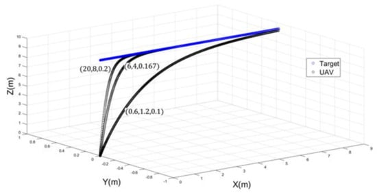
Figure 2. UAV performance for different values of ${\delta }_a,{\delta }_b$, and ${\delta }_c.(i=j=k=2)$.

The figure shows that the fastest response was achieved with the highest values of ${\delta }_a,{\delta }_b$, and ${\delta }_c$, which are 20, 8, and 0.2, respectively. As a result, these values are used in the subsequent simulation to determine the ideal values of $i$, $j$, and $k$. The second part of the simulation shows the performance of the UAV in tracking a moving target in a 3D environment by changing the values of $i$, $j$, and $k$. The target was moving at an acceleration of $\left[\begin{array}{ccc}0.2& 0& 0\end{array}\right] \mathrm{m}/{\mathrm{s}}^2$. In the initial attempt, the value of $i$ was varying between three different values (i.e., 1.5, 2, and 3), while $j$ and $k$ were maintained fixed at the value of 2. Figure 3 shows three different responses of the UAV by varying the value $i$. It is clear that the best performance occurs when $i=2$.

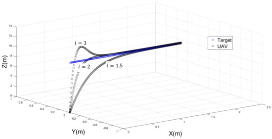
Figure 3. The performance of a UAV when $j=k=2$ with different values of $i$.

Two more simulations were executed in a similar manner—one by modifying the value of $j$ while keeping $i$ and $k$ constant at 2, and a second one by modifying the value of $k$ while keeping $i$ and $j$ constant at 2. Figure 4 shows three UAV trajectories with different values of $j=1.5, 2, 3$, while $i$ and $k$ remain fixed at 2. Figure 5 illustrates the performance of the UAV trajectories with three different values of $k$.

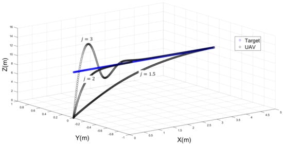
Figure 4. The performance of a UAV when $i=k=2$ with different values of $j$.

Figure 5. The performance of a UAV when $i=j=2$ with different values of $k$.

From the previous simulation runs, the proposed attractive potential field approach for tracking a target in 3D space performed best when ${\delta }_a,{\delta }_b$, and ${\delta }_{c }$= (20, 8, 0.2), and $i=j=k=2$.

4.2. Performance Study on Different Trajectories

More simulations were implemented to investigate the performance of a UAV under various accelerating pathways and different limitations. In all of the following simulations, the previous tuned parameters are used (i.e., ${ \delta }_a,{\delta }_b$, and ${\delta }_{c }$= (20, 8, 0.2), and $i=j=k=2$). Figure 6 illustrates the first challenging scenario, where the UAV was tracking a target accelerating at $\left[\begin{array}{ccc}0.1& 0.1& 0.1\end{array}\right] \mathrm{m}/{\mathrm{s}}^2$. The UAV and target were 10 m apart at the beginning. Despite the fact that they were at different speeds and accelerations, the UAV managed to hit the target.

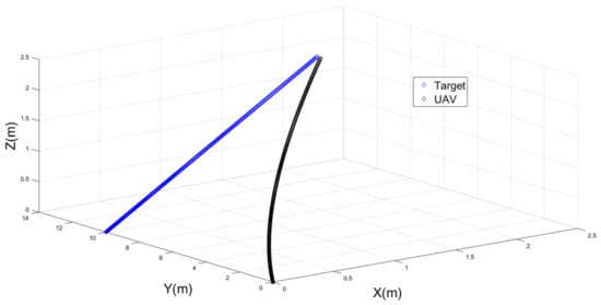
Figure 6. The performance of the UAV in a hard-landing application.

For a target traveling along time-varying acceleration trajectories, it is worthwhile to examine the performance of the attractive force for a UAV in these scenarios. For this purpose, three distinct trajectories (circular, infinite, and helical) are offered to investigate the effectiveness of the proposed method. Figure 7 shows the UAV tracking the target on a circular path. The UAV initiated motion at x = 1 m and y = 0, with zero velocity and acceleration. The target started with velocity $v_x=0, v_y=1 \mathrm{m}/\mathrm{s}$, and acceleration $a_x=-1 \mathrm{m}/{\mathrm{s}}^2, a_y=0 \mathrm{m}/{\mathrm{s}}^2$. The UAV was successfully adjusting to join the trajectory and accurately track the target. The UAV was able to track the target’s velocity in less than one second and its acceleration in two seconds, as shown in Figure 8 and Figure 9.

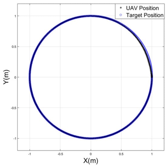
Figure 7. The performance of the UAV to follow a target on a circular trajectory.

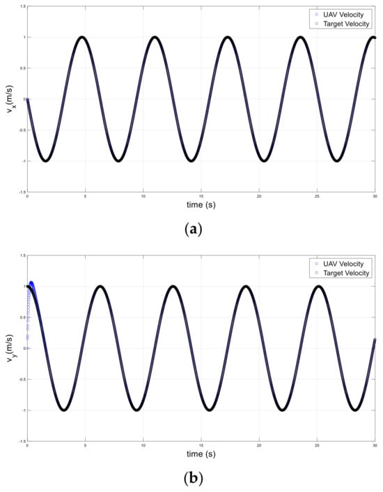
Figure 8. Velocities of the drone and target on a circular path; (a) x-axis, (b) y-axis.

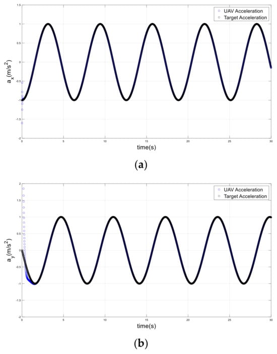
Figure 9. Accelerations of the drone and target on a circular path; (a) x-axis, (b) y-axis.

The infinite trajectory scenario is illustrated in Figure 10, Figure 11 and Figure 12. The UAV initiated motion at x = 0 m and y = 0, with zero velocity and acceleration. The target started with velocity $v_x=-1, v_y=1 \mathrm{m}/\mathrm{s}$, and acceleration $a_x=a_y=0$. The attractive force was rapidly adjusting to give extremely responsive path tracking. In one second, the UAV was able to accurately align with the desired path.

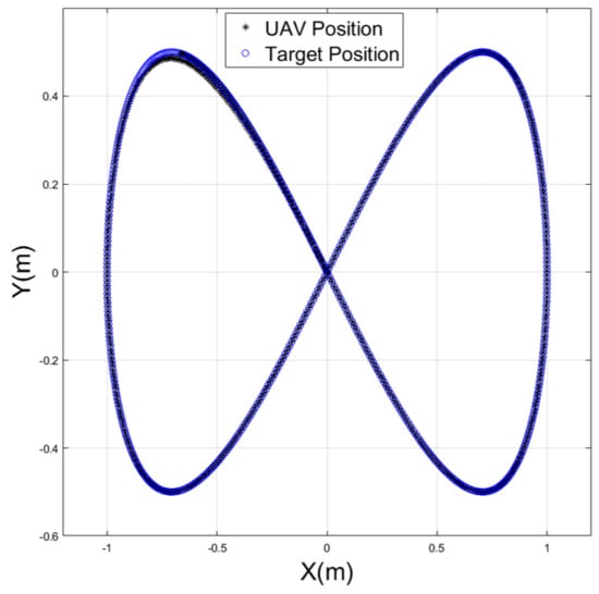
Figure 10. The performance of the UAV to follow a target on an infinite trajectory.

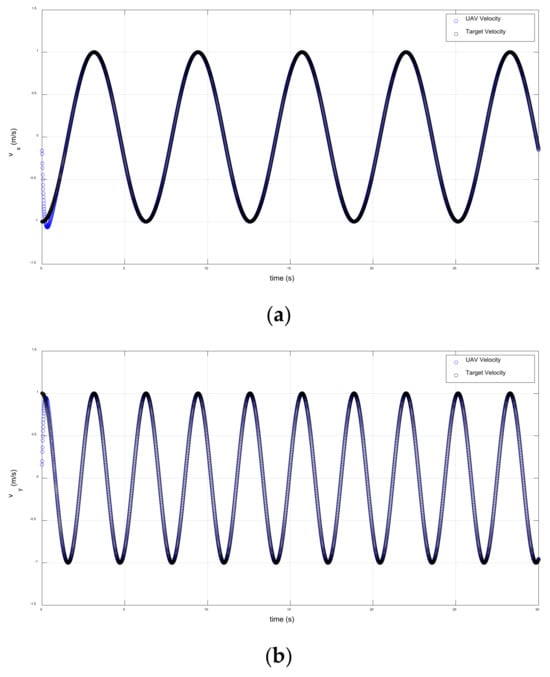
Figure 11. Velocities of the drone and target on an infinite path; (a) x-axis, (b) y-axis.

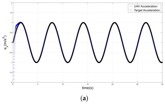
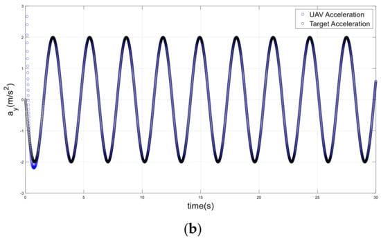
Figure 12. Accelerations of the drone and target on an infinite path; (a) x-axis, (b) y-axis.

To expand the evaluation in the third position, a helical path was tested in another simulation, as shown in Figure 13. In this scenario, the UAV initiated motion at x = 1 m, y = 0, and z = 0, with zero velocity and acceleration. With non-zero velocity and acceleration, the target initiated its motion to move on a helical path with a maximum velocity of $0.5 \mathrm{m}/\mathrm{s}$ and a maximum acceleration of $0.5 \mathrm{m}/{\mathrm{s}}^2$. The UAV was accurately tracking the target along a helical path, as shown in Figure 14 and Figure 15.

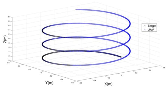
Figure 13. The performance of a UAV to follow a target on a helical trajectory.

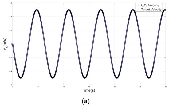
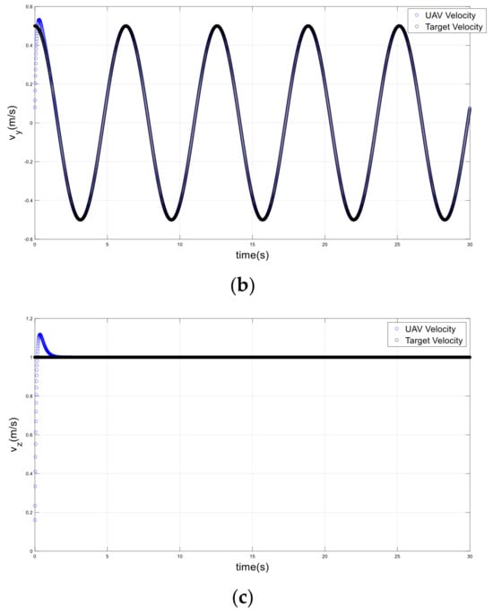
Figure 14. Velocities of the drone and target on a helical path; (a) x-axis, (b) y-axis, (c) z-axis.

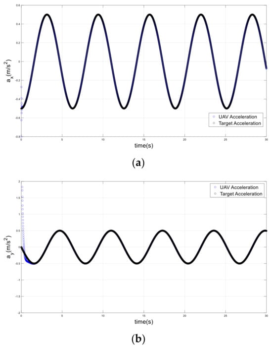
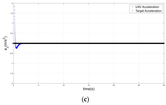
Figure 15. Accelerations of the drone and target on a helical path; (a) x-axis, (b) y-axis, (c) z-axis.

4.3. Performance Study on Edge Cases

More simulation studies are carried out to test the proposed technique in edge circumstances such as sudden stops or abrupt changes in the velocity and acceleration of the target, and disturbances on the UAV while in flight. Figure 16 illustrates a UAV tracking a target on a circular trajectory until it sharply changes direction after completing the circle. Figure 17 and Figure 18 demonstrate a quick shift in velocity and acceleration. The attractive force adapted quickly to this change, providing a faster route to the UAV. The UAV could track the target’s new velocity and acceleration in less than two seconds. Moreover, the UAV successfully and quickly responded to this steering, maintaining a straight route towards the target.

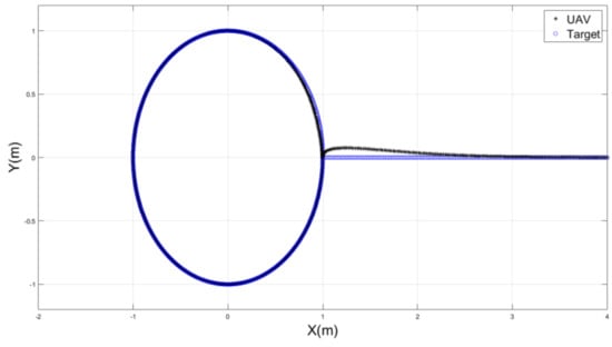
Figure 16. The performance of a UAV throughout sudden steering on the target path.

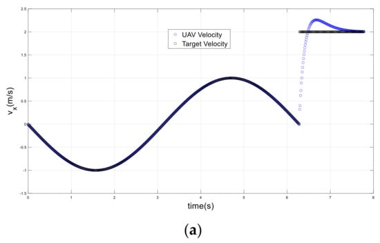
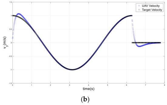
Figure 17. UAV and target velocities in a sudden direction change scenario; (a) x-axis, (b) y-axis.

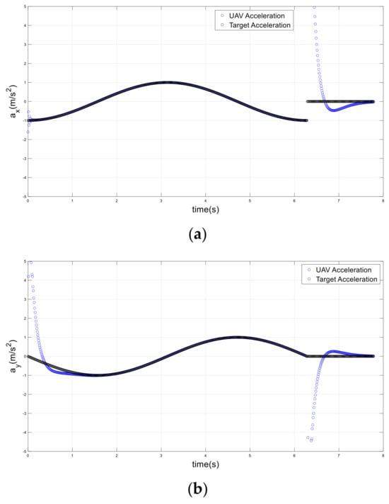
Figure 18. UAV and target accelerations in a sudden direction change scenario; (a) x-axis, (b) y-axis.

Another simulation was run, whereby the UAV goes in a circular path tracking a target, as shown in Figure 19. After completing a quarter circle, the target suddenly came to a complete stop. The UAV responded to the rapid change by decelerating dramatically, as shown in Figure 20 and Figure 21. The UAV then approached the target at zero velocity and acceleration in 1.5 s.

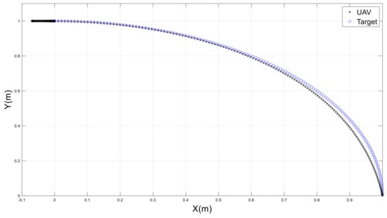
Figure 19. The performance of a UAV tracking a target on a circular path and then stopping.

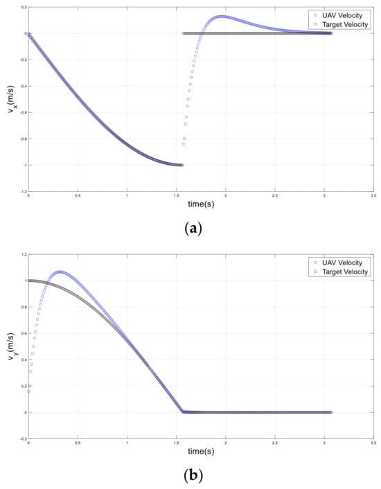
Figure 20. UAV and target velocities in a sudden stop scenario; (a) x-axis, (b) y-axis.

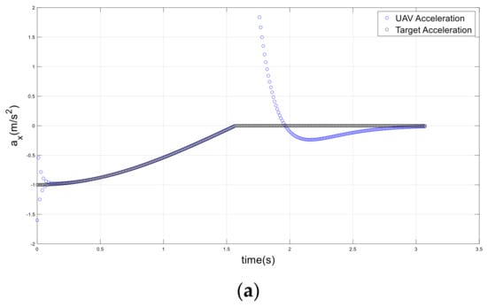
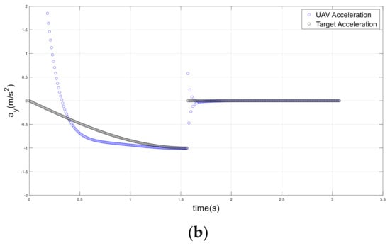
Figure 21. UAV and target accelerations in a sudden stop scenario; (a) x-axis, (b) y-axis.

The last simulation is carried out to examine the performance of the UAV when it is subjected to a disturbance of a stochastic force while it is following a target on a circular trajectory. Starting at position x = 1 and y = 0, the UAV tracked a target on a circular path with initial zero velocities and accelerations. After completing a quarter circle, a disturbance of a stochastic force of 120 N was applied for 0.3 s when the UAV was at y = 1 and x = 0, as shown in Figure 22. The UAV effectively adapted to this change and resumed its circular flight within one second. The UAV returned to accurately track the target’s velocity and acceleration, as seen in Figure 23 and Figure 24.

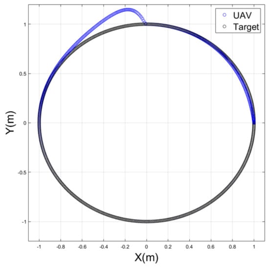
Figure 22. The response of a UAV to an external force while tracking a target on a circular path.

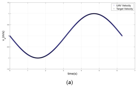
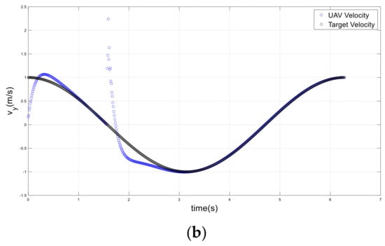
Figure 23. UAV and target velocities in an applied disturbance scenario; (a) x-axis, (b) y-axis.

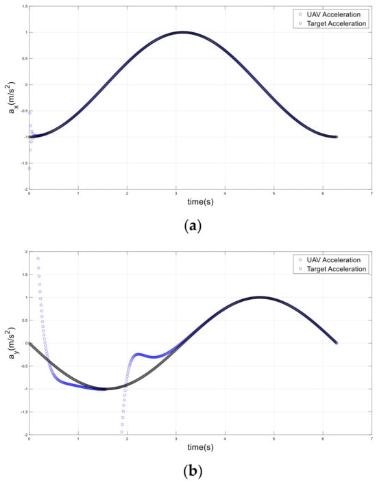
Figure 24. UAV and target accelerations in an applied disturbance scenario; (a) x-axis, (b) y-axis.

5. Experimental Setup and Results

The proposed potential field path planning method was evaluated using Qdrone from Quanser (Markham, ON, Canada), as well as an internal motion tracking system from Vicon (Oxford, UK), as shown in Figure 25. The system accurately positions a moving body, such as a drone, in 3D space. The cameras of the Vicon system are sensitive to all light in their spectrum, which might result in data noise. This would lead to inaccuracy in marker tracking, lowering the quality of motion capture data. However, the system has addressed these issues by incorporating proper noise filters. A computer was used as a ground control station (GCS) to perform the network and computing tasks. Simulink R2024 was used to implement the drone–computer communications, Vicon–computer communications, and control implementations, all using Quanser’s Quarc toolbox.

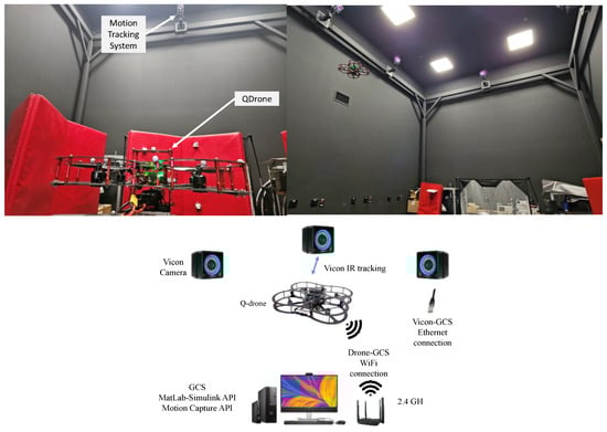
Figure 25. Experimental Setup of Qdrone and the Vicon motion tracking system.

The goal of the experiments is to assess the performance of the proposed path planning system, which was improved by the acceleration term, and to compare it to the performance of the conventional potential field method, which only proposes the position and velocity components. To ensure fair comparisons, each experiment began at the same time and location. The motion of the drone was tested to follow a virtual target along defined paths of positions, velocities, and accelerations. Various path scenarios (i.e., circular, infinite, and helical) have been proposed to examine the efficiency of drone motion. The suggested path planning approach is integrated as a high-level controller that arranges the UAV route. The adopted drone was tested using a robust low-level controller, as stated in [1]. This controller demonstrated robustness against several types of disturbances.

Accurate position, velocity, and acceleration measurements are required to properly implement both acceleration-improved and conventional potential field path-planning. Position measurements from the Vicon system were used directly because of their high accuracy, which is deemed to be 0.02 mm by the manufacturer. To obtain accurate velocity and acceleration estimates, the measurements from the motion tracking system and the drone’s inertial measurement unit (IMU) were fused using a complementary filter as used in [1,33], as follows:

$$\left\{\begin{array}{c}\widehat{a}=k_1\left(v-\widehat{v}\right)+g{e}_3+Qa\\ \dot{Q}=QS\left(\Omega -b\right)+k_v\left(v-\widehat{v}\right)a^T\\ \widehat{v}=v+{\displaystyle \frac{1}{2}}\int \left(Qa+g{e}_3\right)+k_2\left(p-\widehat{p}\right)\end{array}\right.$$

(20)

where $\widehat{a}$ and $\widehat{v}$ are the estimated accelerations and velocities, respectively. $v$ and $p$ are the velocity and position of the drone, respectively. The actual positions and velocities were determined using the indoor motion-tracking system. $k_1$, $k_2$, and $k_v$ are positive gains of the filter. $Q\in {\mathbb{R}}^{3\times 3}$ is a virtual rotation matrix and $\Omega$ is the angular speed measured by the gyroscope. The gyroscope measurements were corrected using gyro bias $b$. The local gravity vector in the inertial frame was given by $g{e}_3={\left[\begin{array}{ccc}0& 0& g\end{array}\right]}^T.$

For all the experimental scenarios that used the improved acceleration-based potential field, the optimized attractive force parameters were as follows:

$$\left\{\begin{array}{c}i=2\\ j=2\\ k=2\end{array}\right.$$

(21)

$$\left\{\begin{array}{c}{\delta }_a=20\\ {\delta }_b=8\\ {\delta }_c=0.2\end{array}\right.$$

(22)

These parameters were obtained in a manner similar to that of the simulation process, as discussed in Section 4.1. To make fair comparisons with the conventional potential field method, the optimized parameters were determined by [17], as follows:

$$\left\{\begin{array}{c}i=2\\ j=2 \end{array}\right.$$

(23)

$$\left\{\begin{array}{c}{\delta }_a=35\\ {\delta }_b=10\end{array}\right.$$

(24)

In a circular path scenario, the target was moving in a 1.5 m circle at a height of 1 m. Furthermore, the target should move at velocities of [−0.4, 0.4] m and an acceleration of [−0.1, 0.1] $\mathrm{m}/{\mathrm{s}}^2$. Figure 26a,b show how the drone tracked the target while accounting for and ignoring the acceleration term, respectively.

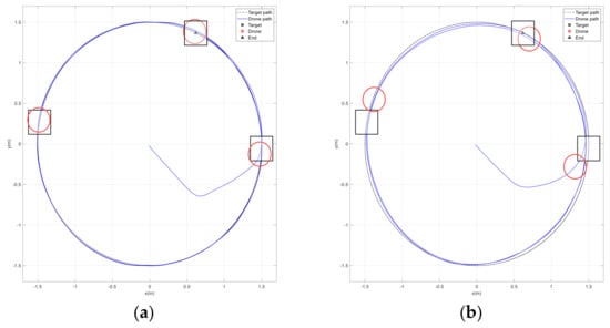
Figure 26. Circular path tracking. (a) Improved potential field with acceleration. (b) Conventional potential field.

The drone was able to transition from the origin to the target more efficiently and quickly than the conventional method, as shown in Figure 27, Figure 28 and Figure 29. The drone accurately tracked the target’s position, speed, and acceleration, allowing for a more accurate landing. It is worth noting that the short-period spikes seen on some curves were due to Vicon drone miss coverage at certain points. Consequently, when the drone entered an area not covered by cameras, the Vicon system provided less accurate positioning, as shown in Figure 28b.

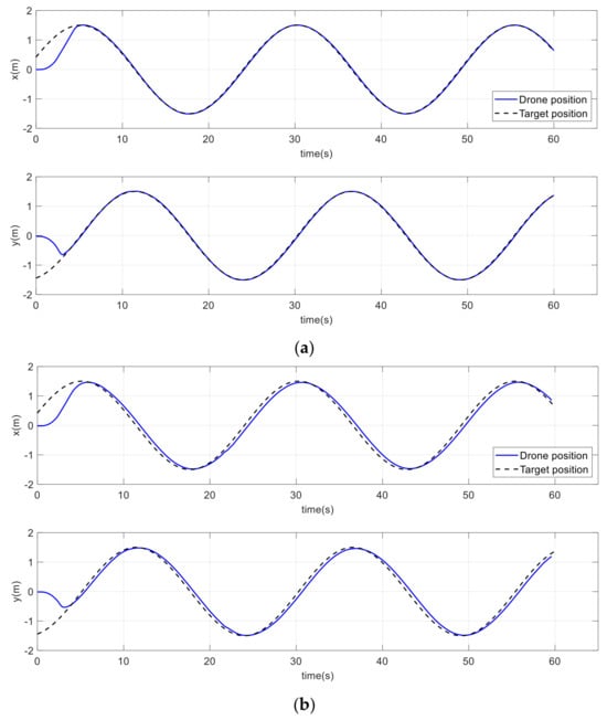
Figure 27. Drone and target positions on a circular path. (a) Improved method. (b) Conventional method.

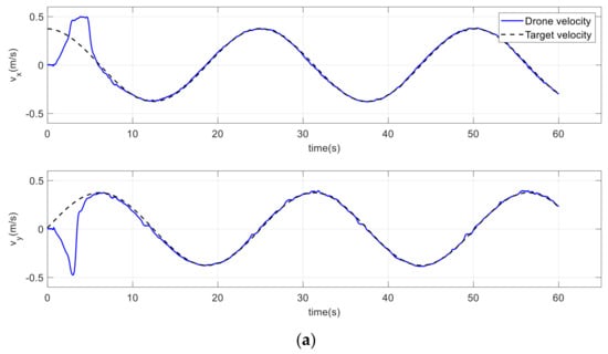
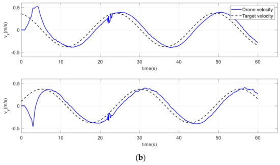
Figure 28. Drone and target velocities on a circular path. (a) Improved method. (b) Conventional method.

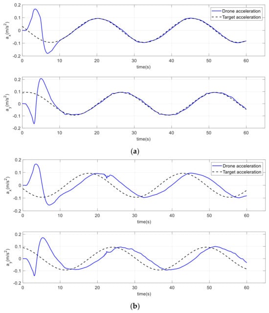
Figure 29. Drone and target accelerations on a circular path. (a) Improved method. (b) Conventional method.

Table 2 shows the mean square error (MSE) of positions, velocities, and accelerations for both approaches. The table clearly shows how the drone path was improved using the proposed method compared to the conventional potential field. The performance of the drone path with the conventional method lagged behind that of the improved approach in terms of position, velocity, and acceleration, with percentage differences of 54.45%, 48.73%, and 53.15%, respectively.

Table 2. MSE of position, velocity, and acceleration for the two methods on a circular path.

	$\mathit{x} \mathbf{\left(}\mathbf{m}\mathbf{\right)}$	$\mathit{y} \mathbf{\left(}\mathbf{m}\mathbf{\right)}$	${\mathit{v}}_{\mathit{x}} \mathbf{\left(}\mathbf{m}\mathbf{/}\mathbf{s}\mathbf{\right)}$	${\mathit{v}}_{\mathit{y}} \mathbf{\left(}\mathbf{m}\mathbf{/}\mathbf{s}\mathbf{\right)}$	${\mathit{a}}_{\mathit{x}} \mathbf{\left(}\mathbf{m}\mathbf{/}{\mathbf{s}}^{\mathbf{2}}\mathbf{\right)}$	${\mathit{a}}_{\mathit{y}} \left(\mathbf{m}/{\mathbf{s}}^2\right)$
Improved method	0.0320	0.0536	0.0064	0.0102	0.0020	0.0023
Conventional method	0.0881	0.1050	0.0146	0.0184	0.0047	0.0045
Difference % (between the two methods)	54.45		48.73		53.15

In another scenario, the drone must follow the infinite path depicted in Figure 30. With similar gains, the Figure shows that the performance of the drone path using the proposed method was significantly better than that of the conventional method. Figure 31, Figure 32 and Figure 33 demonstrate how the drone maintained accurate tracking of the position, velocity, and acceleration along the infinite path. The acceleration term in the potential field attractive force enables the drone to quickly compensate for the shortage of position and velocity terms. Again, due to the limited space size, one or two Vicon cameras missed the drone coverage. As a result, the drone oscillated for a relatively very short period, as shown in certain figures.

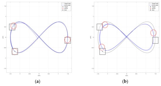
Figure 30. Infinite path tracking. (a) Improved potential field with acceleration. (b) Conventional potential field.

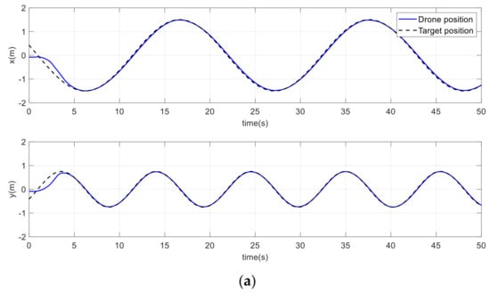
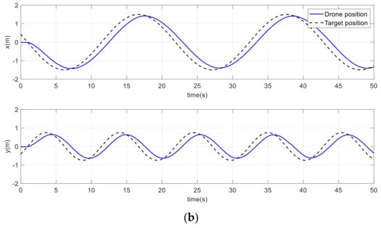
Figure 31. Drone and target positions on an infinite path. (a) Improved method. (b) Conventional method.

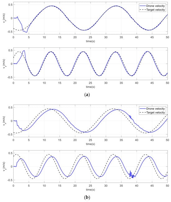
Figure 32. Drone and target velocities on an infinite path. (a) Improved method. (b) Conventional method.

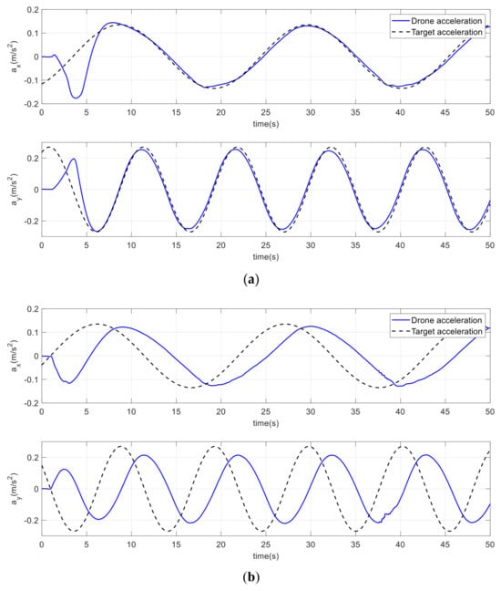
Figure 33. Drone and target accelerations on an infinite path. (a) Improved method. (b) Conventional method.

The proposed method performed better for drone positioning on an infinite path. Table 3 shows that the improved method has a significantly lower MSE for position, velocity, and acceleration than the conventional method. The table also shows the significant differences between the two methods.

Table 3. MSE of position, velocity, and acceleration for the two methods on an infinite path.

	$\mathit{x} \mathbf{\left(}\mathbf{m}\mathbf{\right)}$	$\mathit{y} \mathbf{\left(}\mathbf{m}\mathbf{\right)}$	${\mathit{v}}_{\mathit{x}} \mathbf{\left(}\mathbf{m}\mathbf{/}\mathbf{s}\mathbf{\right)}$	${\mathit{v}}_{\mathit{y}} \mathbf{\left(}\mathbf{m}\mathbf{/}\mathbf{s}\mathbf{\right)}$	${\mathit{a}}_{\mathit{x}} \mathbf{\left(}\mathbf{m}\mathbf{/}{\mathbf{s}}^{\mathbf{2}}\mathbf{\right)}$	${\mathit{a}}_{\mathit{y}} \mathbf{\left(}\mathbf{m}\mathbf{/}{\mathbf{s}}^{\mathbf{2}}\mathbf{\right)}$
Improved method	0.0066	0.0041	0.0088	0.0086	0.0018	0.0052
Conventional method	0.0952	0.0745	0.0209	0.0324	0.0082	0.0539
Difference % (between the two methods)	93.57		68.09		89.9

To expand the evaluation of performance in 3D space, the virtual target was moving along a helical path. As shown in Figure 34a, the drone was accurately positioned over the target in three directions and performed better than the conventional method, owing to the improved potential field attractive force. Over a helical path of a 1.5 m radius, the drone tracked the target position more accurately, as shown in Figure 35a. Furthermore, the drone reached the target’s velocity and acceleration with very small differences, as shown in Figure 36a and Figure 37a, respectively.

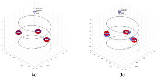
Figure 34. Helical path tracking. (a) Improved potential field with acceleration. (b) Conventional potential field.

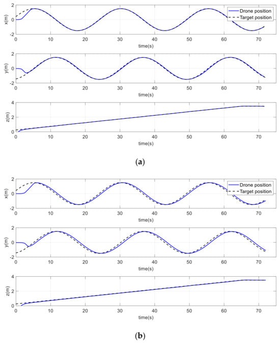
Figure 35. Drone and target positions on a helical path. (a) Improved method. (b) Conventional method.

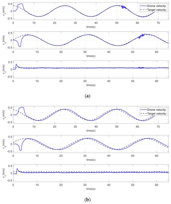
Figure 36. Drone and target velocities on a helical path. (a) Improved method. (b) Conventional method.

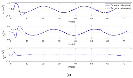
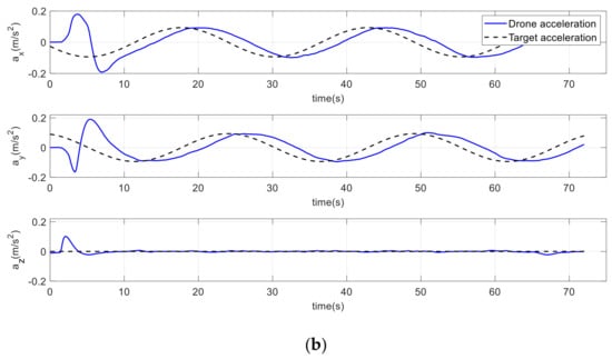
Figure 37. Drone and target accelerations on a helical path. (a) Improved method. (b) Conventional method.

Table 4 shows the MSE in the positions, velocities, and accelerations for the drone on a helical path using the two methods. The improved potential field method outperformed the conventional potential field. The table also shows how the drone path is improved by approximately 200% over the conventional method along all three axes.

Table 4. MSE of position, velocity, and acceleration for the two methods on a helical path.

	$\mathit{x}$ $\mathbf{\left(}\mathbf{m}\mathbf{\right)}$	$\mathit{y}$ $\mathbf{\left(}\mathbf{m}\mathbf{\right)}$	$\mathit{z}$ $\mathbf{\left(}\mathbf{m}\mathbf{\right)}$	${\mathit{v}}_{\mathit{x}}$ $\mathbf{\left(}\mathbf{m}\mathbf{/}\mathbf{s}\mathbf{\right)}$	${\mathit{v}}_{\mathit{y}}$ $\mathbf{\left(}\mathbf{m}\mathbf{/}\mathbf{s}\mathbf{\right)}$	${\mathit{v}}_{\mathit{z}}$ $\mathbf{\left(}\mathbf{m}\mathbf{/}\mathbf{s}\mathbf{\right)}$	${\mathit{a}}_{\mathit{x}}$ $\mathbf{\left(}\mathbf{m}\mathbf{/}{\mathbf{s}}^2\mathbf{\right)}$	${\mathit{a}}_{\mathit{y}}$ $\mathbf{\left(}\mathbf{m}\mathbf{/}{\mathbf{s}}^{\mathbf{2}}\mathbf{\right)}$	${\mathit{a}}_{\mathit{z}}$ $\mathbf{\left(}\mathbf{m}\mathbf{/}{\mathbf{s}}^{\mathbf{2}}\mathbf{\right)}$
Improved PF	0.0236	0.0478	0.0017	0.0057	0.0091	0.0011	0.0017	0.0020	0.0002
Conventional method	0.0636	0.0830	0.0034	0.0127	0.0157	0.0042	0.0044	0.0041	0.0004
Difference % (between the two methods)	49.02			47.67			56.32

Table 5 shows the rising times for each path using both approaches. The data clearly illustrate that the proposed ABPF method achieved a faster response of UAV than the conventional PF. As a result, the UAV could merge with the target path 1.5 s faster for the circular path, 1.6 s for the infinite paths, and 1.3 s for the helical path. The experiments for each scenario utilizing the suggested ABPF approach are also demonstrated in videos that can be found in the Supplementary Materials.

Table 5. Rising time for both methods in different paths.

	Axis	Circular Path (s)	Infinite Path (s)	Helical Path (s)
Conventional PF	x	5.18	6.28	4.89
	Y	3.41	4.08	3.32
	Z	-	-	3.31
Improved PF	X	3.79	4.71	4.26
	Y	3.00	3.77	3.16
	Z	-	-	2.05

6. Conclusions

This paper proposes a novel method for an attractive potential field model that considers the relative acceleration, velocity, and position between a UAV and a target in a highly dynamic path. The new model was developed and deployed in several accelerated path scenarios for soft UAV landings. The generated path of the UAV using the proposed method was compared with that generated by the classic PF method under comparable conditions. The UAV’s performance was evaluated in simulated and experimental scenarios, including complex trajectories such as circular, infinite, and helical trajectories. In terms of the accuracy of the average position, velocity, and acceleration, the proposed PF approach outperformed the classical approach by approximately 50% on the circular and helical paths. Furthermore, the performance of the UAV utilizing the developed method surpassed 67% in the infinite path under similar conditions. The proposed ABPF approach provides a more responsive motion to integrate with the target path than the classic PF. Furthermore, the attractive force was adapted effectively in edge circumstances, such as unexpected pauses or sudden direction changes of the target, as well as to disturbances. The proposed technique only looked at the attractive force of the potential field for an accelerating target. Therefore, the repulsive force for accelerated obstacles could be derived in future works for the free-collision path of the UAV. Furthermore, future directions could include discussing the applicability of the ABPF method in real-world outdoor conditions or assessing its effectiveness on various UAV platforms.

References

- Hayajneh, M.; Al Mahasneh, A. Guidance, Navigation and Control System for Multi-Robot Network in Monitoring and Inspection Operations. Drones 2022, 6, 332. [Google Scholar] [CrossRef]
- Yang, Y.; Xiong, X.; Yan, Y. UAV Formation Trajectory Planning Algorithms: A Review. Drones 2023, 7, 62. [Google Scholar] [CrossRef]
- Liu, L.; Yao, J.; He, D.; Chen, J.; Huang, J.; Xu, H.; Wang, B.; Guo, J. Global dynamic path planning fusion algorithm combining jump-A* algorithm and dynamic window approach. IEEE Access 2021, 9, 19632–19638. [Google Scholar] [CrossRef]
- Dobrevski, M.; Skočaj, D. Dynamic Adaptive Dynamic Window Approach. IEEE Trans. Robot. 2024, 40, 3068–3081. [Google Scholar] [CrossRef]
- Kobayashi, M.; Motoi, N. Local path planning: Dynamic window approach with virtual manipulators considering dynamic obstacles. IEEE Access 2022, 10, 17018–17029. [Google Scholar] [CrossRef]
- Pengfei, J.; Yu, C.; Aihua, W.; Zhenqian, H.; Yichong, W. Optimal Path Planning for Multi-UAV Based on Pseudo-spectral Method. In Proceedings of the 2020 International Conference on Big Data, Artificial Intelligence and Internet of Things Engineering (ICBAIE), Fuzhou, China, 12–14 June 2020; pp. 417–422. [Google Scholar]
- Li, J.; Xiong, Y.; She, J.; Wu, M. A path planning method for sweep coverage with multiple UAVs. IEEE Internet Things J. 2020, 7, 8967–8978. [Google Scholar] [CrossRef]
- Xia, Q.A.L.S.; Guo, M.; Wang, H.; Zhou, Q.; Zhang, X. Multi-UAV trajectory planning using gradient-based sequence minimal optimization. Robot. Auton. Syst. 2021, 137, 103728. [Google Scholar] [CrossRef]
- Li, S.; Chen, Y.; Yang, Y. Multi-rotor UAV path planning based on Model Predictive Control and Control Barrier Function. In Proceedings of the 36th Chinese Control and Decision Conference (CCDC), Xi’an, China, 25–27 May 2024; pp. 1141–1146. [Google Scholar]
- Wu, W.; Li, J.; Wu, Y.; Ren, X.; Tang, Y. Multi-UAV Adaptive Path Planning in Complex Environment Based on Behavior Tree. In Proceedings of the International Conference on Collaborative Computing: Networking, Applications and Worksharing, Shanghai, China, 16–18 October 2020; pp. 494–505. [Google Scholar]
- Tran, N.Q.H.; Prodan, I.; Grøtli, E.I.; Lefèvre, L. Potential-field constructions in an MPC framework: Application for safe navigation in a variable coastal environment. IFAC-Pap. 2018, 51, 307–312. [Google Scholar] [CrossRef]
- Li, J.; Sun, J.; Liu, L.; Xu, J. Model predictive control for the tracking of autonomous mobile robot combined with a local path planning. Meas. Control. 2021, 54, 1319–1325. [Google Scholar] [CrossRef]
- Chen, X.; Zhang, J. The three-dimension path planning of UAV based on improved artificial potential field in dynamic environment. In Proceedings of the 5th International Conference on Intelligent Human-Machine Systems and Cybernetics, Hangzhou, China, 26–27 August 2013; Volume 2, pp. 144–147. [Google Scholar]
- Chengqing, L.; Ang, M.H.; Krishnan, H.; Yong, L.S. Virtual obstacle concept for local-minimum-recovery in potential-field based navigation. In Proceedings of the IEEE International Conference on Robotics and Automation. Symposia Proceedings, Paris, France, 31 May–31 August 2020; Volume 2, pp. 983–988. [Google Scholar]
- Zou, X.-Y.; Zhu, J. Virtual local target method for avoiding local minimum in potential field based robot navigation. J. Zhejiang Univ. Sci. A 2003, 4, 264–269. [Google Scholar] [CrossRef]
- Garibeh, M.H.; Jaradat, M.A.; Alshorman, A.M.; Hayajneh, M.; Younes, A.B. A real-time fuzzy motion planning system for unmanned aerial vehicles in dynamic 3D environments. Appl. Soft Comput. 2024, 150, 110995. [Google Scholar] [CrossRef]
- Garibeh, M.H.; Alshorman, A.M.; Jaradat, M.A.; Ahmad, B.Y.; Khaleel, M. Motion planning of unmanned aerial vehicles in dynamic 3D space: A potential force approach. Robotica 2022, 40, 3604–3630. [Google Scholar] [CrossRef]
- Yao, P.; Wang, H.; Su, Z. Real-time path planning of unmanned aerial vehicle for target tracking and obstacle avoidance in complex dynamic environment. Aerosp. Sci. Technol. 2015, 47, 269–279. [Google Scholar] [CrossRef]
- Khatib, O. Real-time obstacle avoidance for manipulators and mobile robots. Int. J. Robot. Res. 1986, 5, 90–98. [Google Scholar] [CrossRef]
- Ge, S.S.; Cui, Y.J. Dynamic motion planning for mobile robots using potential field method. Auton. Robot. 2002, 13, 207–222. [Google Scholar] [CrossRef]
- Garibeh, M.H.; Jaradat, M.A.K.; Rawashdeh, N.A. A potential field simulation study for mobile robot path planning in dynamic environments. In Proceedings of the 20th International Conference on Research and Education in Mechatronics (REM), Wels, Austria, 23–24 May 2019; pp. 1–8. [Google Scholar]
- Jayaweera, H.M.; Hanoun, S. A dynamic artificial potential field (D-APF) UAV path planning technique for following ground moving targets. IEEE Access 2020, 8, 192760–192776. [Google Scholar] [CrossRef]
- Hayajneh, M.R.; Badawi, A.R.E. Automatic UAV wireless charging over solar vehicle to enable frequent flight missions. In Proceedings of the 3rd International Conference on Automation, Control and Robots, Prague, Czech Republic, 11–13 October 2019; pp. 44–49. [Google Scholar]
- Yu, W.; Lu, Y. UAV 3D environment obstacle avoidance trajectory planning based on improved artificial potential field method. J. Phys. Conf. Ser. 2021, 1885, 022020. [Google Scholar] [CrossRef]
- Keyu, L.; Yonggen, L.; Yanchi, Z. Dynamic obstacle avoidance path planning of UAV Based on improved APF. In Proceedings of the 5th International Conference on Communication, Image and Signal Processing (CCISP), Chengdu, China, 13–15 November 2020; pp. 159–163. [Google Scholar]
- Jayaweera, H.M.; Hanoun, S. Path planning of unmanned aerial vehicles (UAVs) in windy environments. Drones 2022, 6, 101. [Google Scholar] [CrossRef]
- Thangaraj, M.; Sangam, R.S. Intelligent UAV path planning framework using artificial neural network and artificial potential field. Indones. J. Electr. Eng. Comput. Sci. 2023, 29, 1192. [Google Scholar] [CrossRef]
- Feng, J.; Zhang, J.; Zhang, G.; Xie, S.; Ding, Y.; Liu, Z. UAV dynamic path planning based on obstacle position prediction in an unknown environment. IEEE Access 2021, 9, 154679–154691. [Google Scholar] [CrossRef]
- Du, Y.; Zhang, X.; Nie, Z. A real-time collision avoidance strategy in dynamic airspace based on dynamic artificial potential field algorithm. IEEE Access 2019, 7, 169469–169479. [Google Scholar] [CrossRef]
- BinKai, Q.; Mingqiu, L.; Yang, Y.; XiYang, W. Research on UAV path planning obstacle avoidance algorithm based on improved artificial potential field method. J. Phys. Conf. Ser. 2021, 1948, 012060. [Google Scholar] [CrossRef]
- Ortner, R.; Kurmi, I.; Bimber, O. Acceleration-aware path planning with waypoints. Drones 2021, 5, 143. [Google Scholar] [CrossRef]
- Yin, L.; Yin, Y.; Lin, C.-J. A new potential field method for mobile robot path planning in the dynamic environments. Asian J. Control 2009, 11, 214–225. [Google Scholar] [CrossRef]
- Hayajneh, M.; Melega, M.; Marconi, L. Design of autonomous smartphone based quadrotor and implementation of navigation and guidance systems. Mechatronics 2018, 49, 119–133. [Google Scholar] [CrossRef]
Disclaimer/Publisher’s Note: The statements, opinions and data contained in all publications are solely those of the individual author(s) and contributor(s) and not of MDPI and/or the editor(s). MDPI and/or the editor(s) disclaim responsibility for any injury to people or property resulting from any ideas, methods, instructions or products referred to in the content. |
© 2025 by the authors. Licensee MDPI, Basel, Switzerland. This article is an open access article distributed under the terms and conditions of the Creative Commons Attribution (CC BY) license (https://creativecommons.org/licenses/by/4.0/).