Optimal Layout Planning of Electric Vehicle Charging Stations Considering Road–Electricity Coupling Effects

Abstract

With the advancement of dual-carbon goals and the construction of new types of power systems, the proportion of electric vehicle charging stations (EVCSs) in the coupling system of power distribution and transportation networks is gradually increasing. However, the surge in charging demand not only causes voltage fluctuations and a decline in power quality but also leads to tension in the power grid load in some areas. The complexity of urban road networks further increases the challenge of charging station planning. Although laying out charging stations in areas with high traffic flow can better meet traffic demands, it may also damage power quality due to excessive grid load. In response to this problem, this paper proposes an optimized layout plan for electric vehicle charging stations considering the coupling effects of roads and electricity. By using section power flow to extract dynamic data from the power distribution network and comparing the original daily load curves of the power grid and electric vehicles, this paper plans reasonable capacity and charging/discharging schemes for EVCSs. It considers the impact of the charging and discharging characteristics of EVCSs on the power grid while satisfying the peak-shaving and valley-filling regulation benefits. Combined with the traffic road network, the optimization objectives include optimizing the voltage deviation, transmission line margin, network loss, traffic flow, and service range of charging stations. The Gray Wolf Optimizer (GWO) algorithm is used for solving, and the optimal layout plan for electric vehicle charging stations is obtained. Finally, through road–electricity coupling network simulation verification, the proposed optimal planning scheme effectively expands the charging service range of electric vehicles, with a coverage rate of 83.33%, alleviating users’ charging anxiety and minimizing the impact on the power grid, verifying the effectiveness and feasibility of the proposed scheme.

1. Introduction

With the increase in the scale of electric vehicles (EVs) accessing the power grid, the proportion of electrical vehicle charging stations (EVCSs) accessing the power grid is also constantly rising [1]. This is bound to cause fluctuations in the power grid load curve and affect the stable operation of the power grid [2]. Therefore, research on the location planning of EVCS is of crucial importance. Ref. [3] predicts the spatiotemporal distribution of urban EV charging loads within a day, and then builds EVCSs at specific nodes based on the prediction results. Ref. [4] takes the construction cost of the charging station as the objective, divides a certain area into three regions, and uses the 2m Point Estimation method (2m PEM) to build EVCSs at appropriate locations in each region. Ref. [5] proposes a charging and discharging scheme to reduce the impact of the disorderly charging of a large number of EVs on the power grid. Through time-of-use transaction electricity prices, the charging and discharging periods of EVs are guided to achieve the effect of peak shaving and valley filling. Ref. [6] addresses the road–electricity coupling network and EV charging issues, and plans EVCSs with the goal of taking into account the installation of EVCS operators, the demands of EV users, and reducing the annual social cost of the distribution network. Ref. [7] takes the minimum total annual cost of the charging station as the objective and uses an improved immune clone selection algorithm for the capacity determination and grid connection of EVCSs. Ref. [8] considers the comprehensive cost of the charging station layout and the penalty measures for violating the power grid constraints, extracts the best functions of two algorithms (Chicken Swarm Optimization (CSO) and Teaching–Learning-Based Optimization (TLBO)), and plans the location of EVCSs. Ref. [9] takes the minimum cost of the charging station and the economic loss of users as the objective, and conducts location planning of EVCS through an improved particle swarm algorithm. Ref. [10] aims at maximizing the revenue of the charging station and minimizing the fluctuation of the interaction power between the charging station and the distribution network, and dynamically adjusts the electricity price to achieve orderly charging and discharging of EVs.

Most of the above studies do not consider the energy storage characteristics of EVCSs, that is, the discharging capacity to the power grid. Refs. [3,4,6,7,8,9] all treat EVCSs as loads for site selection without considering the discharging capacity of EVCSs. Refs. [5,10] consider the impact of some EV discharging characteristics on the power grid, but they all achieve orderly charging and discharging of EVs by adjusting the electricity price and use the interaction of EVs and EVCSs to achieve the goal of peak shaving and valley filling. If the charging and discharging capacity of an EVCS is only constrained and adjusted by the electricity price, then the volatility is too large, and the EVCS is not regarded as a distributed power source, and the impact of the charging station as a power source on the power grid is not considered. The planning of EVCSs in most of the above studies is mostly aimed at the lowest economic cost, and less consideration is given to the impact of EVCSs accessing the power grid.

Through analysis and comparison, the optimal location planning scheme for electric vehicle charging stations (EVCSs) proposed in this paper comprehensively considers the coupling effect of the distribution network and the transportation road network. This scheme not only assesses the impact of EVCS planning on traffic flow and the service range of the charging station but also regards an EVCS as an energy storage unit and deeply analyzes its multi-dimensional impact on the power grid from its charging and discharging behavior, including voltage fluctuation, transmission line margin, network loss, and the regulation benefit based on peak shaving and valley filling. By using the Gray Wolf Optimizer (GWO) for optimization and finding a solution, this scheme can efficiently balance the complex relationship between charging demand and power grid operation and, finally, obtain a reasonable planning scheme that not only meets the traffic flow demand but also minimizes the impact on the power grid. The differences between this article and the conventional methods are presented in Table 1 as follows:

Table 1. Research and analysis comparison table.

Comparative Dimension	Regular Method	Method Proposed in This Article
Goals	Least economic cost	On the basis of reducing economic cost, meeting traffic flow demand and minimizing the impact on the power grid
Characteristics of EVCSs	Load	Negative energy storage unit
Grid impact considerations	Less	Multi-dimensional impact: voltage fluctuation, transmission line margin, network loss, peak cutting and valley filling regulation benefit
EVCS and power grid interaction	Discharge capacity is not considered; interaction is mainly analyzed through electricity price regulation	Considering the effect of charging and discharging behavior on the power grid, EVCS is regarded as a distributed power supply
Planning methods	2m PEM, improved immune clone selection algorithm, CSO, TLBO, particle swarm optimization, etc.	Gray Wolf Optimization (GWO) algorithm
Spatiotemporal distribution prediction	Yes	Yes, considering the coupling effect between the traffic network and distribution network
Economic cost	Aims for minimal costs	Considers the cost, but this is not the only goal; pays more attention to the balance between grid operation and traffic flow
Economic losses for users	Not specifically mentioned	Considers user economic losses, with the goal of minimization
Electricity price regulation	Achieves orderly charging and discharging through electricity price regulation	Dynamic adjustment of electricity price to achieve orderly charging and discharging, but this is not the only means
Algorithm optimization	Multiple algorithms, but may not take into account power grids and transportation networks	GWO algorithm, integrated consideration of power grid and transportation network

2. Electric Vehicle Charging Station Model

The magnitude of charging demand is closely related to traffic flow. Suppose there are N_{_JT} nodes in the road network, and the traffic flow passing through the road network node f at time t is 1/S₄. The service range of the m-th EVCS is N_{EVCS_m}, and the specific formulas are described in detail in Section 3.6 and Section 3.7. According to the number of nodes contained in the service range, the total traffic flow of the m-th EVCS can be obtained. Let α be the penetration rate of electric vehicles in the traffic road network, and the number of EVs contained within the service range of the m-th EVCS at time t can be obtained through Equation (1).

$$N_{\mathrm{car}\_\mathrm{t}\_\mathrm{m}}=\alpha {\displaystyle \sum _{n_{EVCS\_m}=1}^{N_{EVCS\_m}}\frac{1}{S_{4,t,n_{EVCS\_m}}}}$$

(1)

where N_{car_t_m} is the number of EVs included in the service area of the m-th EVCS at time t, and S_{4,t,nEVCS_m} is the traffic flow of the n_{EVCS_m} node in the service area of the m-th EVCS at time t.

In real life, not all N_{car_t_m} vehicles need to be charged. In this paper, the travel demand of EVCSs is calculated based on the travel patterns of various EVs, and EVs are classified. The specific travel patterns of various vehicles are shown in Table 2 [11].

Table 2. The initial charging time and SOC of various vehicles.

	Initial Charge Time	Initial SOC
Electric buses	23:00–5:30 the next day	Follow the normal distribution N (0.5, 0.12)
Electric taxis	23:00–7:00 the next day 11:00–18:00	Follow the normal distribution N (0.35, 0.12)
Electric official cars and special vehicles	22:00–5:00 the next day	Follow the normal distribution N (0.6, 0.12)
Electric private cars	Working hours: 8:00–17:00 18:00–7:00 the next day	Follow the normal distribution N (0.7, 0.12)

Using Table 2 and the Monte Carlo sampling process, the number of electric vehicles connected at time t is defined as follows [12]:

$$P(n_{EV,t})={\displaystyle \frac{e^{-{\lambda }_{EV,t}}\times {\lambda }_{EV,t}^{n_{EV,t}}}{n_{EV,t}!}}$$

(2)

where λ_EV,t is the expected value of the number of EVs at time t, and n_EV,t is the number of EVs randomly accessing. The characteristic function is

$$\mathrm{\Psi }(t)=\exp \{{\lambda }_{EV,t}(e^{it}-1)\}$$

(3)

The charging load is calculated at an interval of 10 min, with a total of 144 points in a day. The total charging load is as follows:

$$P_t={\displaystyle \sum _{n=1}^{N_{-EV}}{P}_{n,t}}$$

(4)

where P_t is the total charging power in the t-th time period, where t = 1, 2, …, 144; N_{_EV} is the total number of EVs in the t-th time period; and P_{n, t} is the charging load of the n-th vehicle in the t-th time period.

The calculation steps of the EVCS charging load are presented as follows:

(1)

Input parameters such as the battery capacity and variance of the EV, and calculate the number N of EVs at the i-th moment of the EVCS;

(2)

Classify the EVs at the i-th moment in accordance with the distribution of the starting charging time.

(3)

Based on the distribution of the initial state of charge (SOC) of various types of EV batteries, randomly generate the initial SOC, and calculate the required charging capacity in accordance with Equation (5):

$$P=C(1-SOC)$$

(5)

where C is the battery capacity of the EV and P is the charging power of the EV.

(4)

Return to the second step and repeat the aforementioned steps to acquire the charging load of various types of EVs within a day.

(5)

Superimpose the EV charging load curves to obtain the total charging load curve of the EVCS.

3. Research Scheme of Multi-Objective Optimization for Electric Vehicle Charging Stations Based on Regulatory Benefits

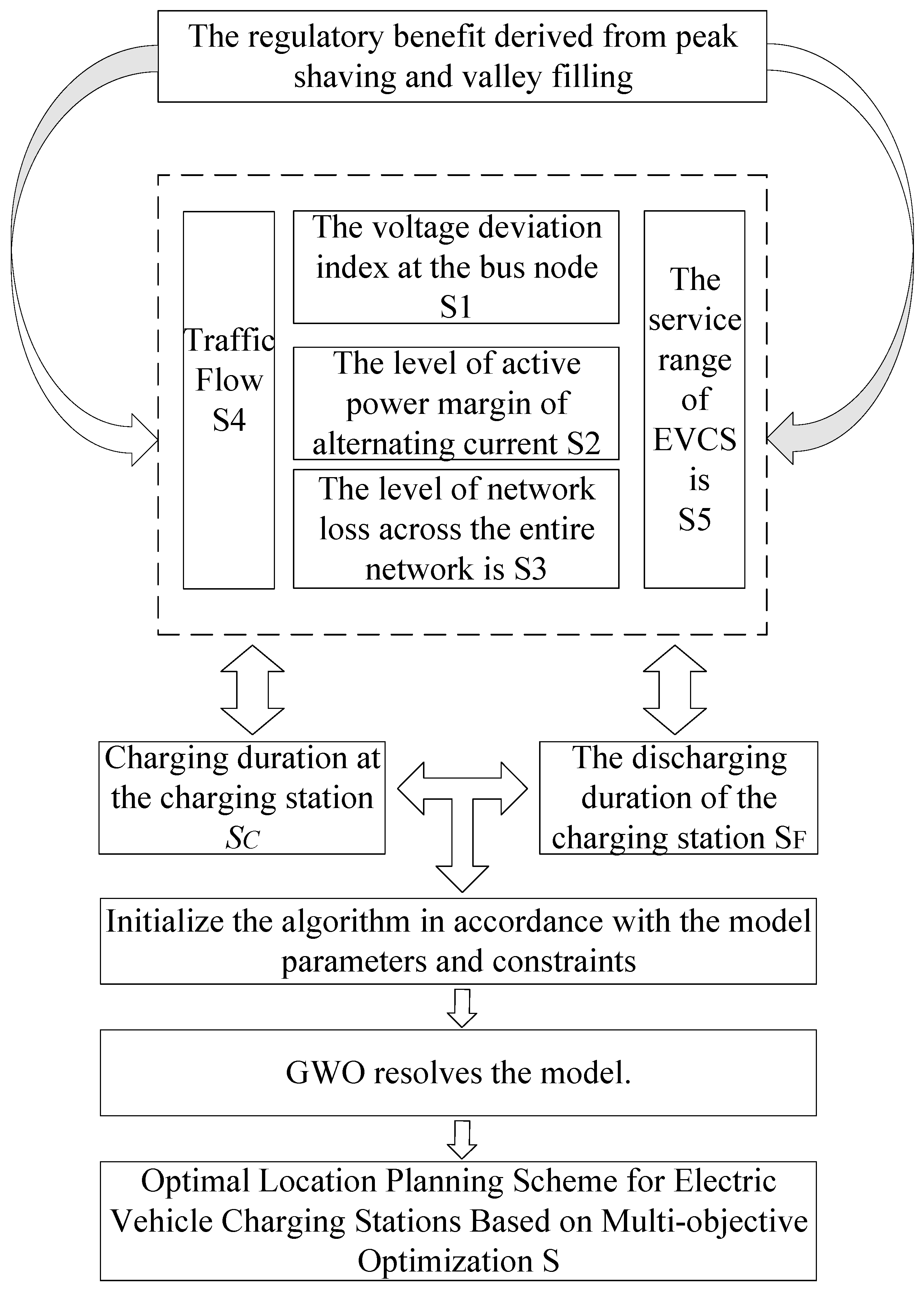
3.1. EVCS Multi-Objective Optimization Scheme

This paper considers the impact of EVCSs on the grid based on the working hours of EVCS and divides it into two cases. The multi-objective optimization function is as follows:

$$S_C=k_1{S}_1+k_2{S}_2+k_3{S}_3+k_4{S}_4+k_5{S}_5$$

(6)

$$S_F=k_6{S}_1+k_7{S}_2+k_8{S}_3+k_9{S}_4+k_{10}{S}_5$$

(7)

$$S=k_{11}{S}_C+k_{12}{S}_F$$

(8)

where S_C and S_F represent the target items addressed by the EVCSs at the charging and discharging instants. S₁, …, S₅ are the sub-targets considered in each target item, and ultimately, they are planned to be solved as a single target through Formula (8). k₁, k₂, …, k₁₂ are the proportion coefficients of the sub-targets in the total target, and ac and af are the weight coefficients, signifying the proportions of the objective functions at the charging and discharging instants in the total objective function, respectively, which can be adjusted based on actual requirements. S₁, S₂, S₃, S₄, and S₅, respectively, denote the voltage deviation of the bus node, the active power margin level of the AC line, the network loss level of the entire network, the traffic flow, and the service range of the charging station, and S is the objective function after considering the charging and discharging capabilities of the EVCS.

In the site planning of EVCSs presented in this paper, it is essential to take into account the weights of each objective function in the comprehensive index. In this paper, the analytic hierarchy process is employed to convert the multi-objective optimization problem into a decision-making issue of a total objective from both quantitative and qualitative perspectives. Firstly, a judgment matrix needs to be constructed. The specific construction method is presented in the following equation:

$$A=\begin{array}{cc}& A_1\hspace{1em}{A}_2\hspace{1em}{A}_3\hspace{1em}{A}_4\\ \begin{array}{l}{A}_1\\ A_2\\ A_3\\ A_4\end{array}& \left[\begin{array}{cccc}{a}_{11}& a_{12}& \dots & a_{1n}\\ a_{21}& a_{22}& \dots & a_{2n}\\ \cdots & \cdots & \cdots & \cdots \\ a_{n1}& a_{n2}& \cdots & a_{nn}\end{array}\right]\end{array}$$

(9)

[A₁, A₂, …, A_n] represent the n-dimensional second-level sub-objectives, and pairwise comparisons are carried out in accordance with Table A3. The weight coefficients of each element are calculated as presented in the following formula:

$$K_i={\displaystyle \frac{\sqrt[n]{{\displaystyle \prod _{j=1}^n{a}_{ij}}}}{{\displaystyle \sum _{i=1}^n\sqrt[n]{{\displaystyle \prod _{j=1}^n{a}_{ij}}}}}}(i=1,2,\cdots ,n)$$

(10)

The expression utilized for the consistency check of matrix A is

$$F_{CR}={\displaystyle \frac{F_{CI}}{F_{RI}}}={\displaystyle \frac{\left({\lambda }_{\max }-n\right)}{(n-1)F_{RI}}}$$

(11)

where λ_max represents the maximum eigenvalue of matrix A, F_CR stands for the consistency ratio, F_CI denotes the consistency index, and F_RI refers to the random index. The specific values are presented in Table A4. If F_CR < 0.1, the weight coefficient is deemed reasonable. If F_CR ≥ 0.1, it implies that the judgment matrix A is inconsistent and requires adjustment. The block diagram of the optimization scheme presented in this paper is depicted in Figure 1:

Figure 1. EVCS optimization strategy flow chart.

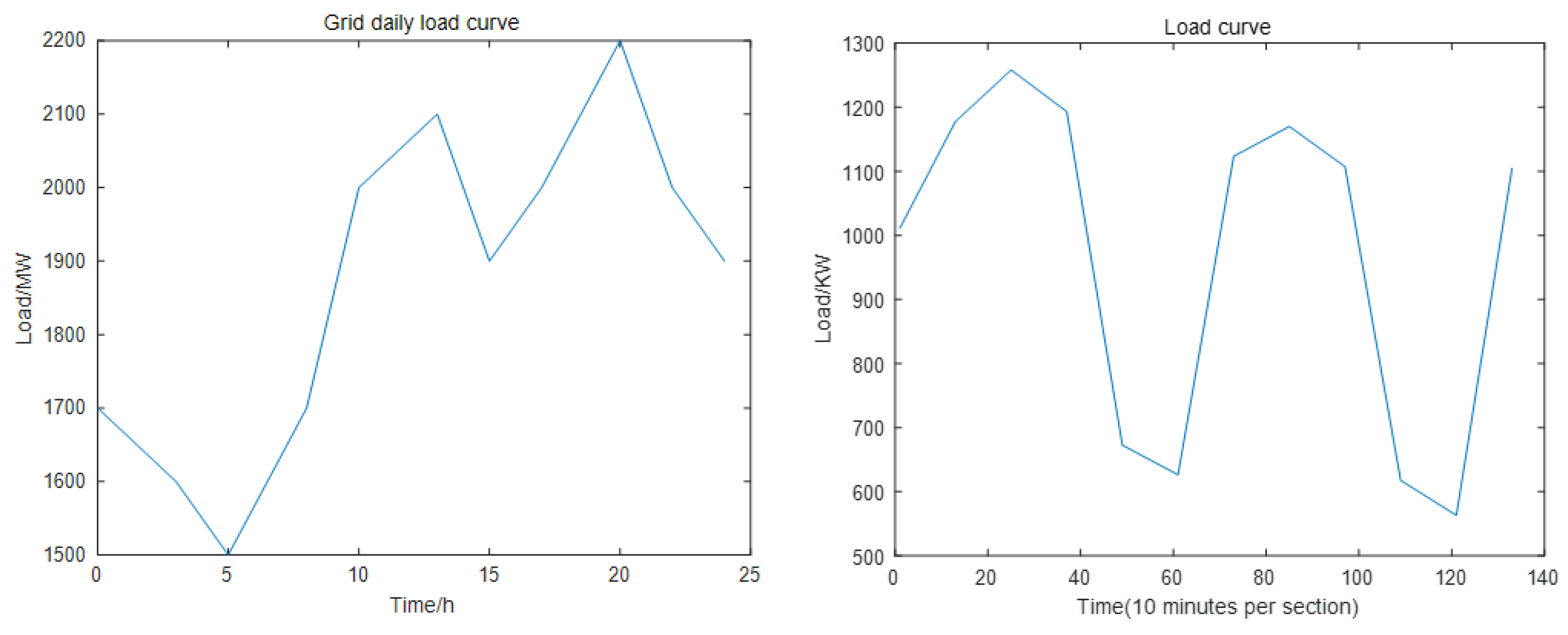
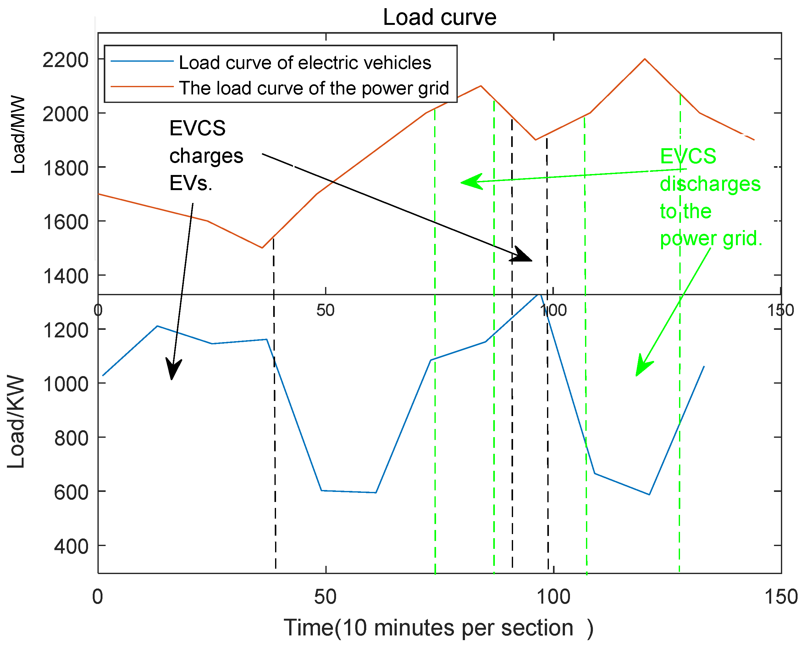
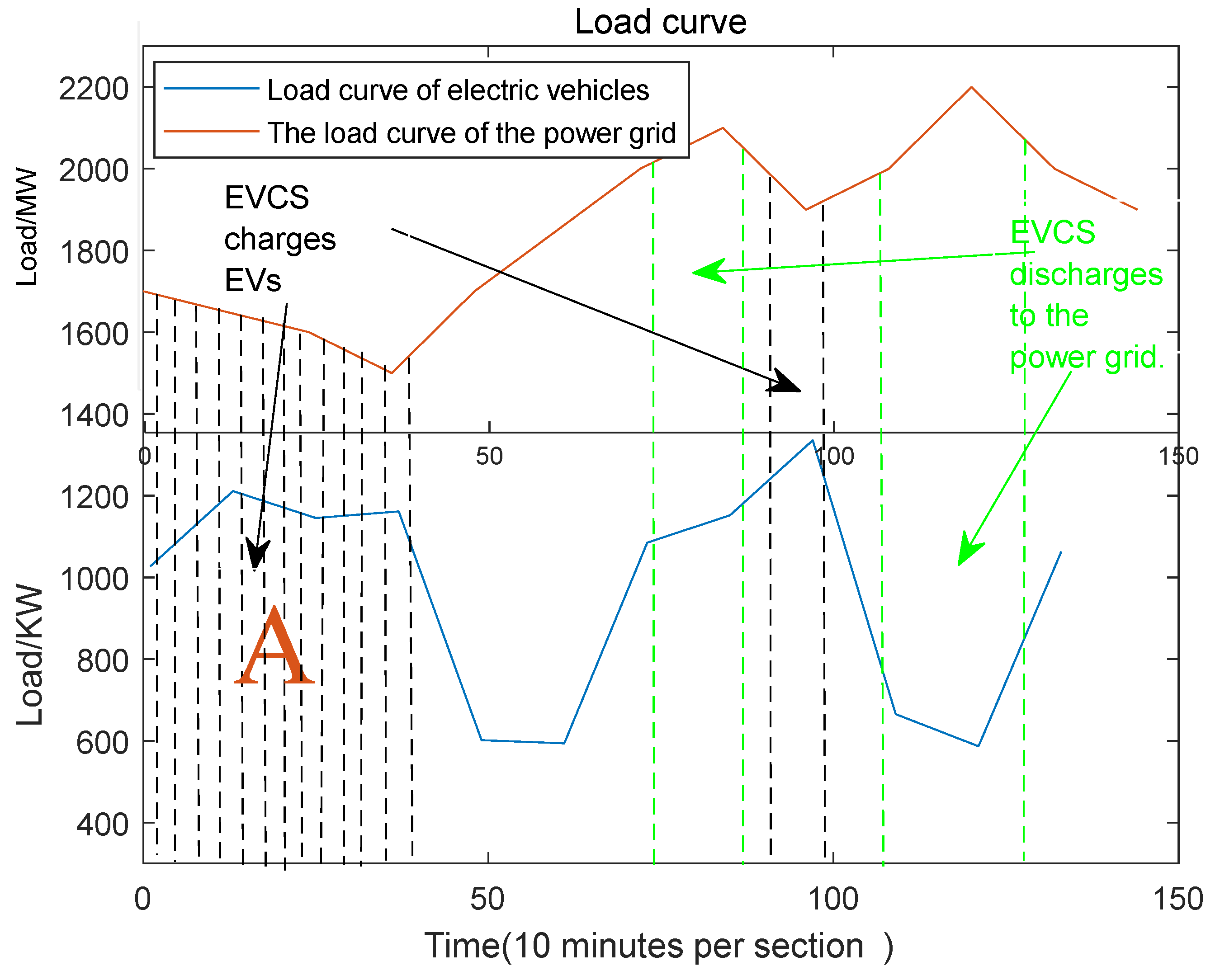
3.2. The Regulatory Benefit Derived from Peak Shaving and Valley Filling

Drawing on Ref. [13], the original daily load data of a regional power grid were investigated and analyzed. The original daily load curve, as depicted in Figure 2, was obtained through MATLAB (2020a) simulation verification.

Figure 2. The original daily load curves of the power grid and electric vehicle charging.

It can be discerned from the aforesaid figure that the troughs of the original daily load curve of the power grid occur from 2:00 to 7:00 and from 14:00 to 17:00, among which 5:00 and 15:00 represent the lowest points; the peaks are, respectively, from 11:00 to 13:00 and from 19:00 to 21:00, among which 12:00 and 20:00 are the highest points. After 23:00, the load curve begins to exhibit a downward trend [14].

Through the EVCS model constructed in Section 1 and the Poisson distribution adhered to by the number of EVs and the normal distribution followed by the charging time of EVs, it can be observed from the aforementioned figure that the troughs of the original daily load curve of EV charging occur from 7:00 to 12:00 and from 18:00 to 21:00; the peaks are, respectively, from 13:00 to 16:00 and from 22:00 to 5:00 of the next day. After 21:00, the load curve begins to exhibit an upward trend. The peak and trough times of the power grid and the load are presented in Table A1 and Table A2. Through Matlab simulation, a comparison diagram of the daily load curve of the power grid and EVs is obtained, and the results are as follows:

In Figure 3, the trough of the daily load curve of the power grid and the peak of the daily load curve of EVs lie within the dotted area indicated by the black arrow, while the peak of the daily load curve of the power grid and the trough of the daily load curve of EVs are encompassed within the dotted area indicated by the green arrow. This implies that the peak electricity consumption time of EVs exhibits a complementary tendency with the electricity consumption peak of the power grid. Hence, this trend can be exploited to reduce the peak–valley difference of the power grid load through an effective charging and discharging scheme of EVCSs.

Figure 3. Comparison of daily load curves between power grid and EVs.

Based on the aforementioned analysis, in this paper, during the trough period of the original daily load curve of the power grid, the EVCS undertakes large-scale charging of EVs. During the remaining periods, some charging piles are enabled for EV charging. During the peak period, the energy storage power supply [15] within the EVCS is discharged. In this manner, the charging demand of EVs can be fulfilled, the load curve of the power grid can be smoothed, and the regulation benefit of the EVCS can also be satisfied, attaining the objective of peak shaving and valley filling. The state of charge at the discharge time of the energy storage battery is presented in the following equation:

$$SO{C}_{-F}=1-{\displaystyle \sum _{t=1}^{T_{-}c}\frac{P_{{\mathrm{disbat}}_{-}t}\Delta t}{E_b}}$$

(12)

where SOC_{_F} indicates the state of charge of the energy storage battery during the discharge period, T_{_c} represents the charging period of the EVCS, P_{disbat_t} denotes the discharge power of the energy storage battery at time period t, Δt represents the time interval, and E_b represents the investment capacity of the energy storage system.

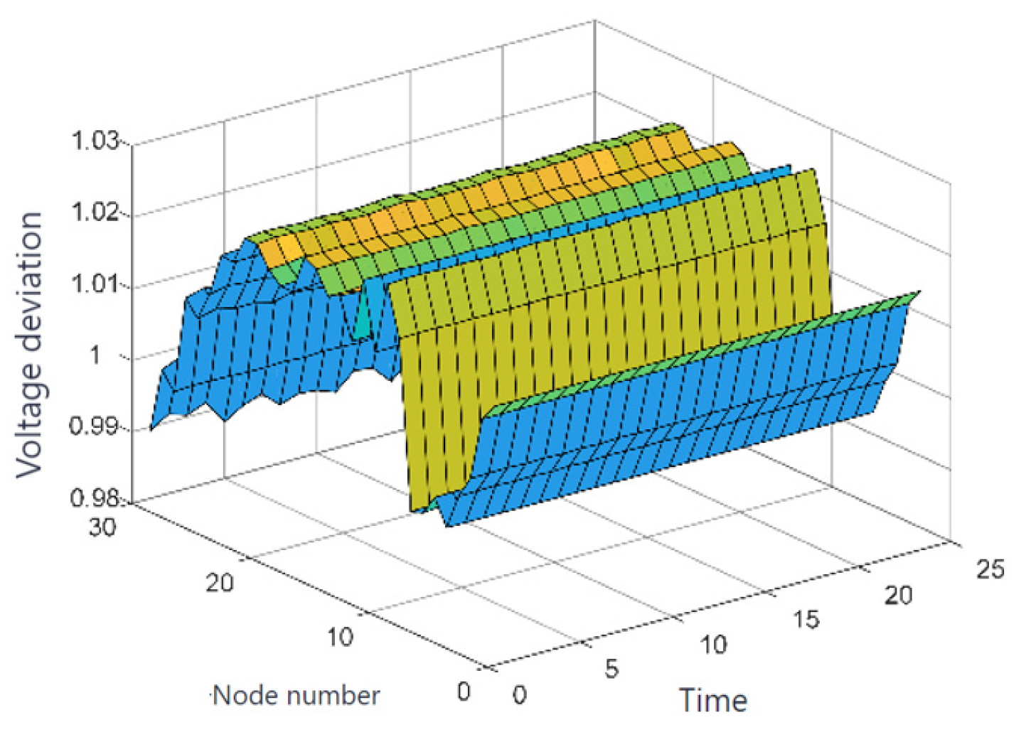
3.3. Index of Voltage Deviation at the Bus Node

In the optimization scheme presented in this paper, when an EV is connected to the distribution network, the bus node voltage should be as proximate as possible to the rated voltage U_N, and the disparity between them is demonstrated as follows [16]:

$$\Delta U_{bus-i,t}=U_{bus-i,t}-U_N$$

(13)

The voltage deviation index proposed in this paper requires considering not only the voltage deviation level of N nodes at time t, but also the degree of node voltage fluctuation. Taking the node voltage deviation considering the voltage fluctuation level as the optimization objective, and ensuring that the voltage deviation of all bus nodes is minimized, it is defined as objective S₁:

$$S_1={\displaystyle \frac{S_{1-a}}{NT}}{\displaystyle \sum _{i=1}^N{\displaystyle \sum _{t=1}^T\frac{(U_{bus-i,t}-U_{bus-i,t,\min })(U_{bus-i,t,\max }-U_{bus-i,t})}{(U_N-U_{bus-i,t,\min })(U_{bus-i,t,\max }-U_N)}}}$$

(14)

$$S_{1-\alpha }=\frac{1}{NT}\sum _{n=1}^N\sum _{n=1}^T|\frac{U_{\mathit{bus}-i,t}}{U_N}-{\overline{U}}_{\mathit{bus}-i}|$$

(15)

$${\overline{U}}_{\mathit{bus}-i}=\frac{1}{T}\sum _{t=1}^T\left|\frac{U_N-U_{\mathit{bus}-i,t}}{U_N}\right|$$

(16)

where N represents the number of nodes in the distribution network; t ∈ T, where T is the hydrogen production time; S_1–a is the voltage fluctuation level index; and ${\overline{U}}_{bus-i}$ represents the average value of the voltage fluctuation level of node i over the calculation period.

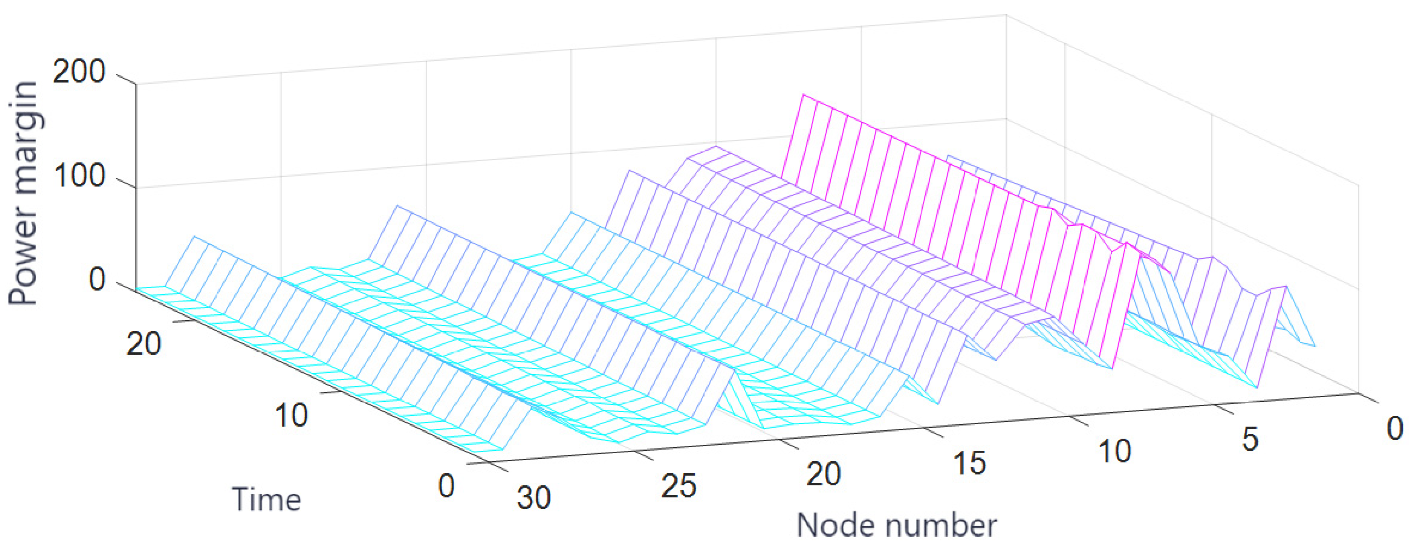
3.4. Active Power Margin Level of AC Power

The active power margin level of alternating current is a crucial indicator for measuring the stable operation of the power system. In this paper, the variance is obtained to reflect the degree of dispersion of the power flow in each line, minimizing the variance of each node as much as possible. The variance value considering power fluctuation and maximum power deviation is taken as the optimization objective and defined as objective S₂, as shown in the following equation:

$$S_2=S_{2-a}\sqrt{{\displaystyle \frac{1}{TK}}{{\displaystyle \sum _{t=1}^T{\displaystyle \sum _{\mathrm{k}=1}^K(P_{EV,t}-P_{k,t})}}}^2}$$

(17)

$$S_{2-a}={\displaystyle \frac{a}{TK}}{\displaystyle \sum _{t=1}^T{\displaystyle \sum _{\mathrm{k}=1}^K(P_{\mathrm{k},\mathrm{t}}-P_{EV,t})}}+{\displaystyle \frac{b}{TK}}{\displaystyle \sum _{t=1}^T{\displaystyle \sum _{\mathrm{k}=1}^K(\frac{P_{\mathrm{k}-\max }-P_{k,t}}{P_{\mathrm{k}-\max }})}}$$

(18)

$$P_{EV}={\displaystyle \frac{{\displaystyle \sum _{t=1}^T{\displaystyle \sum _{\mathrm{k}=1}^K{P}_{\mathrm{k},\mathrm{t}}}}}{TK}}$$

(19)

where P_EV,t represents the average power of the AC line connected to node i at time t; P_k,t represents the active power level of line k connected to node i at time t; S_2–a represents the influence coefficient considering the power fluctuation and the maximum power deviation on the objective function, where a and b, respectively, represent the weights of the power fluctuation and the maximum power deviation in the influence coefficient; P_k-max represents the transmission power upper limit of line k connected to node i at time t, with k ∈ K; and K represents the total number of AC lines connected to node i.

3.5. The Extent of Power Loss Across the Entire Network

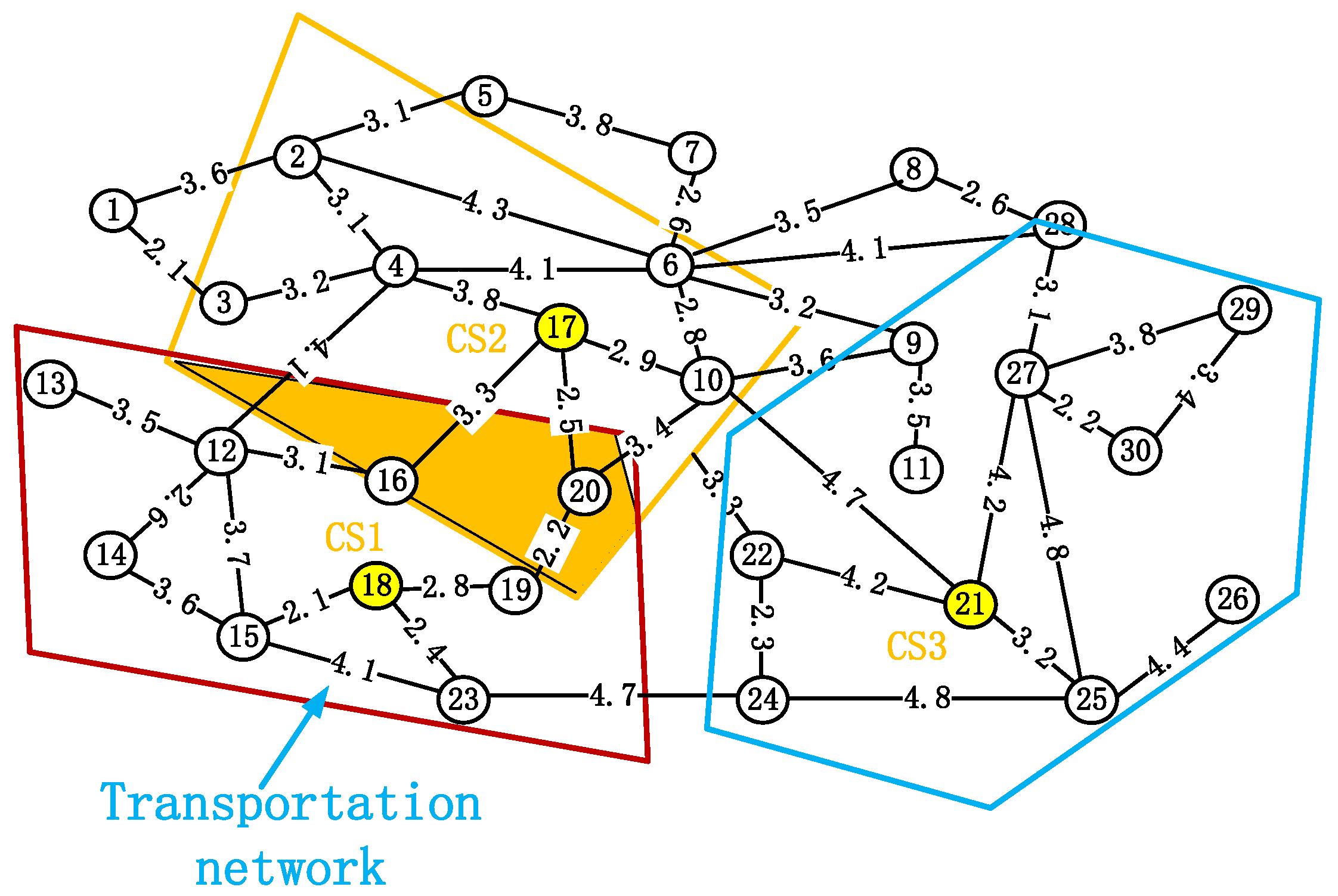
In the operation of power grids, excessive network loss will result in the loss of electrical energy and the waste of energy. Reducing network loss is an important economic objective. The line loss of the system is calculated by the Newton–Raphson method, and the active network loss is expressed as follows [17]:

$$S_3={\displaystyle \sum _{\mathrm{i}=1}^{N_L}{G}_{\mathrm{ij}}\left(U_{\mathrm{i}}^2+U_{\mathrm{j}}^2-2U_{\mathrm{i}}{U}_{\mathrm{j}}\cos ({\theta }_{\mathrm{i}}-{\theta }_{\mathrm{j}})\right)}$$

(20)

where S₃ represents the network loss of the system, where U_i and U_j denote the voltage amplitudes of nodes i and j; G_ij stands for the conductance of the branch between nodes i and j; n_l ∈ N_L, and N_L is the set of transmission lines; and θ_i and θ_j signify the voltage phase angles of nodes i and j.

3.6. Traffic Flux

The layout of EVCS requires considering not only the influence on the power grid but also the constraints of the traffic network in actual circumstances. One of the main entities served by EVCSs is EV users. Hence, the planning scheme of EVCSs needs to capture the traffic flow to the greatest extent possible to meet the actual demands of users. The traffic flow objective function is presented as follows:

$$S_4=1/{\displaystyle \sum _{l=1}^L\frac{F_i{F}_j}{1.5d_{EVC{S}_{-}l}}}\hspace{1em}\forall i,j\in N,i\ne j$$

(21)

where S₄ indicates the objective function of traffic flow, where F_i and F_j are the weights of the two nodes, namely the starting point i and the ending point j of the line, and d_{EVCS_l} represents the length of the path l in the traffic network.

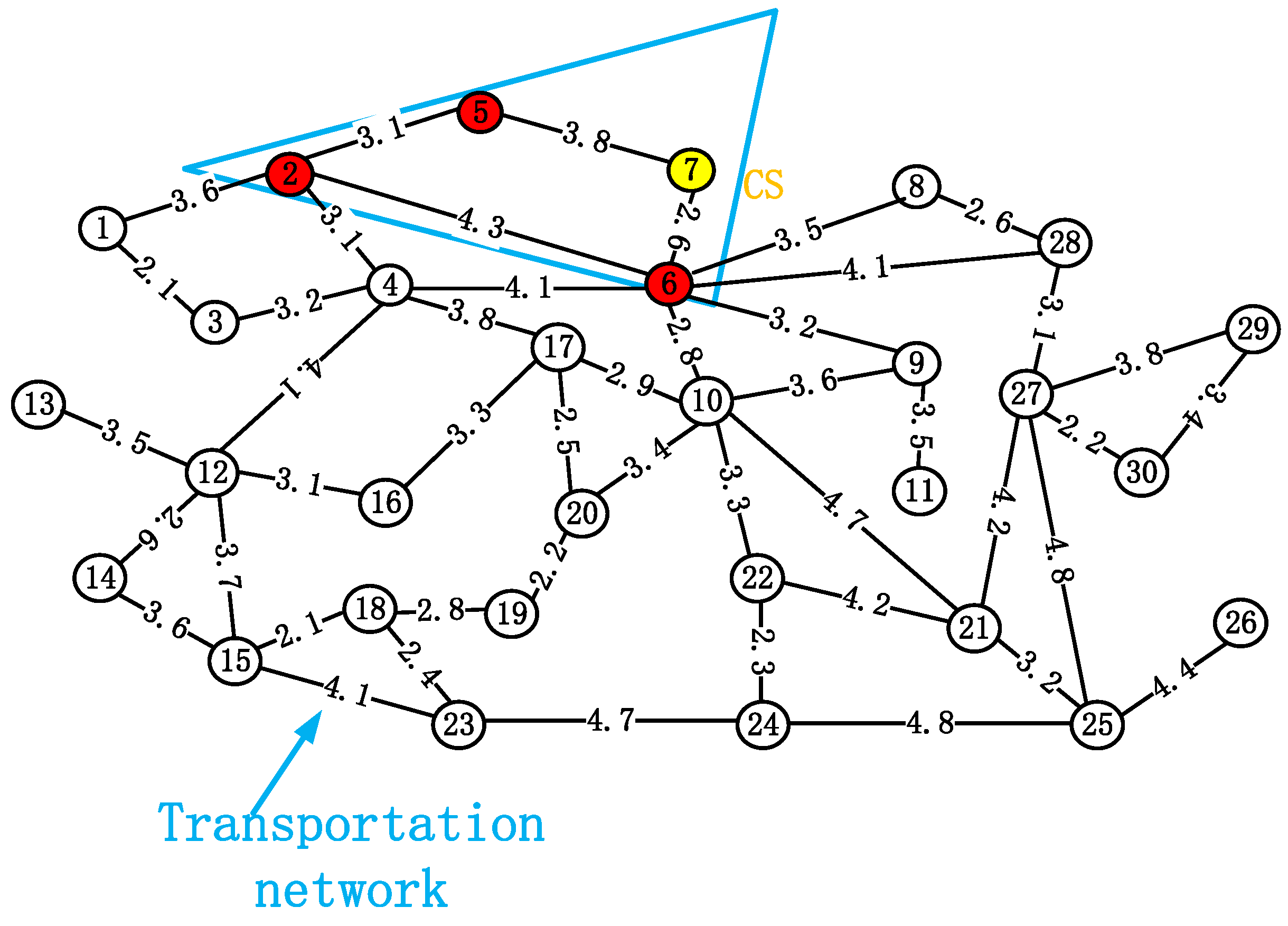
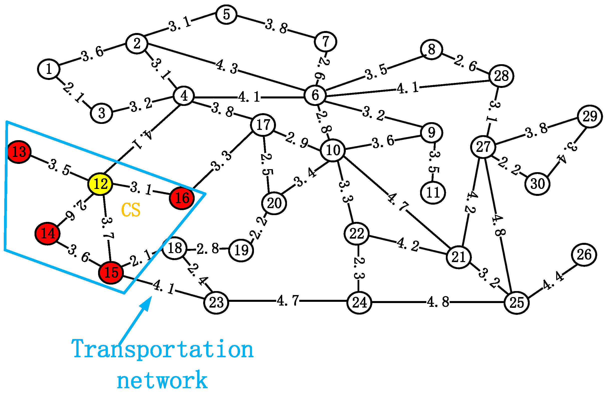
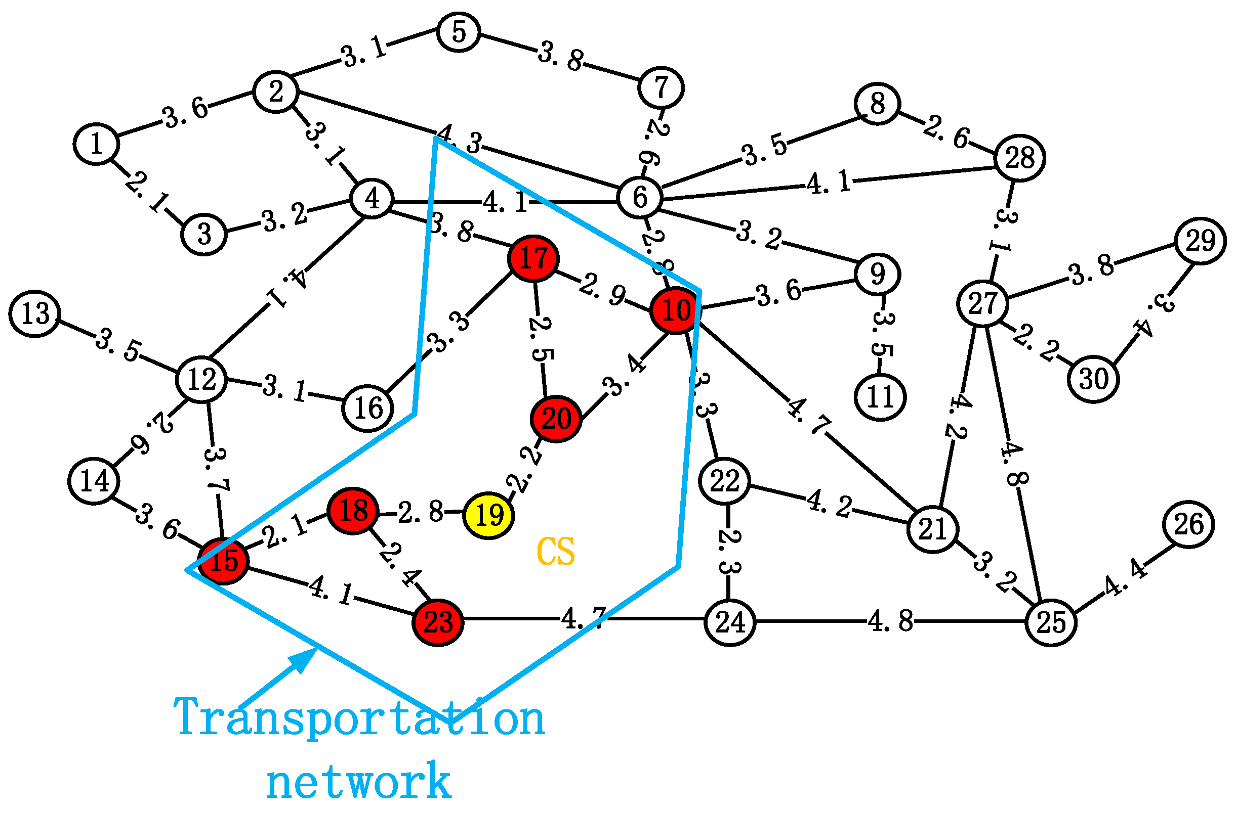
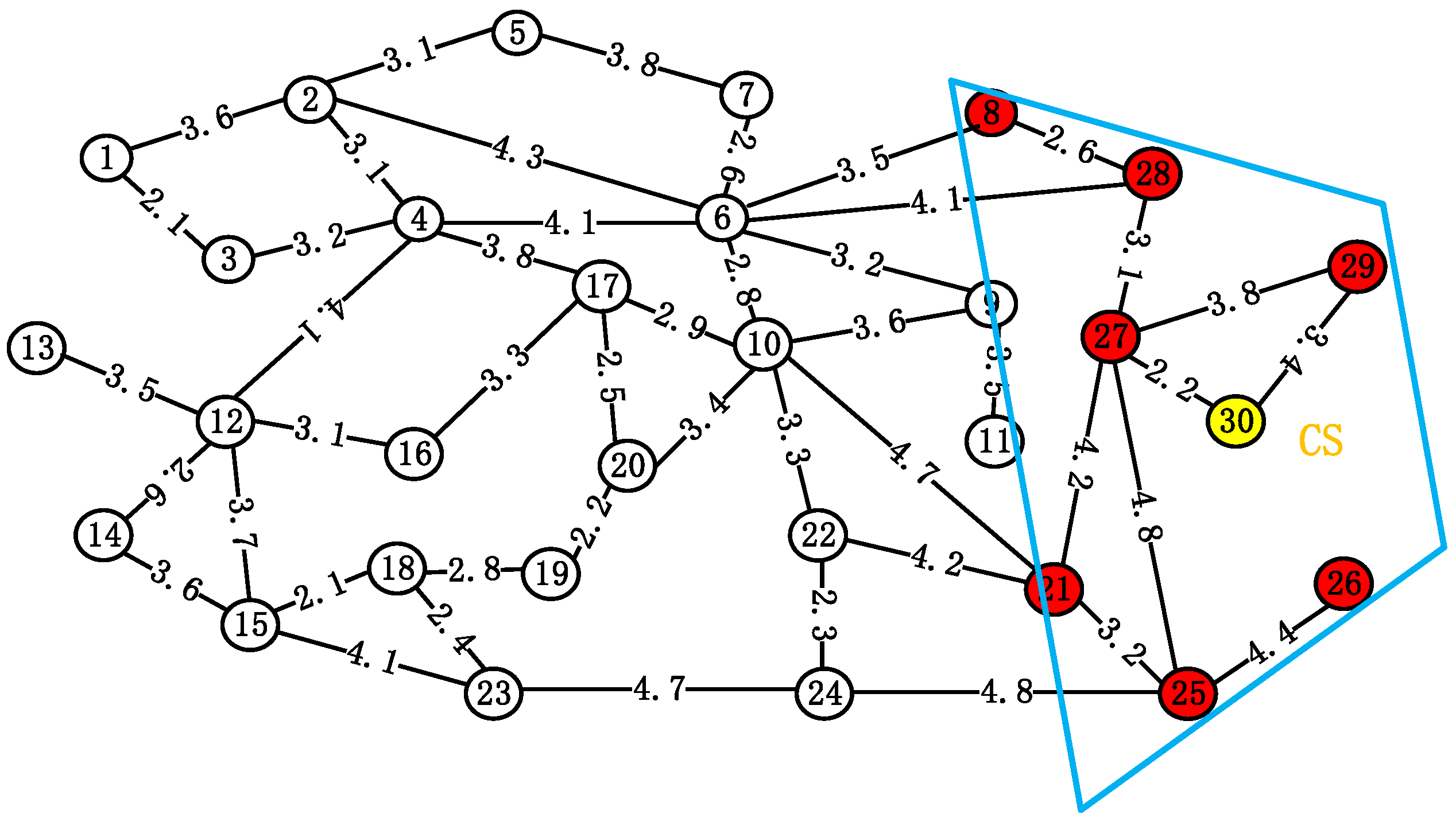
3.7. The Scope of Services Provided by the Charging Station

In the planning scheme presented in this paper, the attractiveness of EVCSs to users should be maximized to the greatest extent possible. Apart from factors such as electricity price and distance, the disparities of each node will also have certain influential factors interfering with the choices of EV users. Therefore, in this paper, the introduction of weight coefficients is employed to reflect the influence of other factors on users. The objective function of the charging range of EVCSs proposed in this paper is presented in the following equation:

$$S_5={\displaystyle \sum _{m=1}^M\frac{\sqrt{\frac{1}{M}{\displaystyle \sum _{m=1}^M{\left(S_{m_{-}cs}-\frac{1}{M}{\displaystyle \sum _{m=1}^M{S}_{m_{-}cs}}\right)}^2}}}{S_{m_{-}cs}-\frac{1}{M}{\displaystyle \sum _{m=1}^M{S}_{m_{-}cs}}}}$$

(22)

where S_{m_CS} denotes the attractiveness of the m-th charging station to EV users. The charging range of EVCSs is preferably larger. In this paper, the planning scheme will be solved by means of GWO. To adapt to the algorithm rules, S₅ represents the reciprocal of the charging range of EVCSs, that is, the smaller S₅ is, the larger the charging range. The attractiveness of the m-th charging station to EV users is presented as follows:

$$S_{m_{-}cs}={\displaystyle \frac{P_{EVC{S}_{-}m}}{{\lambda }_i\left({\displaystyle \sum _{l=1}^L{d}_{EVC{S}_{-}l}}{E}_{EV}{P}_{EV}\right)}}$$

(23)

where P_{EVCS_m} denotes the charging power of the m-th EVCS, λ_i represents the influence weight of other factors at node i, d_{EVCS_l} represents the length of the path l for an electric vehicle to reach the EVCS, E_EV represents the power consumption per unit distance, and P_EV represents the electricity price of the EVCS.

$$N_{EVCS\_m}={\displaystyle \frac{N_{\_JT}}{S_5}}\times 100\%$$

(24)

where N_{EVCS_m} indicates the number of nodes encompassed within the influence scope of the m-th EVCS, and N_{_JT} represents the total number of nodes in the transportation network.

3.8. Constraint Conditions

(1)

Voltage constraints at nodes:

$$U_{i,t\min }\le U_{i,t}\le U_{i,t\max }$$

(25)

where U_i,tmax and U_i,tmin represent the maximum and minimum values of the voltage at node i at time t.

(2)

Constraints on branch capacity:

$$P_{ij}^2+Q_{ij}^2\le S_{ij\max }^2$$

(26)

where P_ij and Q_ij represent the active and reactive powers on the branch, and S_ijmax is the maximum capacity permitted for the branch.

(3)

Constraints on the quantity of EV charging and total demand:

$$N_{E{V}_{-}m}\le N_{EVC{S}_{-}m}$$

(27)

$${\displaystyle \sum _{v=1}^V{S}_{CDZ}\ge {\displaystyle \sum _{n=1}^{N_{EV}}{S}_{EV}}}$$

(28)

where N_{EV_m} represents the charging quantity of EVs in the m-th EVCS, N_{EVCS_m} indicates the number of permitted charging stations in the m-th EVCS, V stands for the quantity of charging piles in the EVCS, S_CDZ denotes the capacity of the charging piles, and S_EV represents the capacity of the EVs.

(4)

Constraint of the power balance equation:

$$\left\{\begin{array}{c}{P}_i+P_{DGi}=P_{Li}+U_i{\displaystyle \sum _{j=1}^N{U}_j}\left(G_{ij}\cos {\theta }_{ij}+B_{ij}\sin {\theta }_{ij}\right)\\ Q_i+Q_{DGi}=Q_{Li}+U_i{\displaystyle \sum _{j=1}^N{U}_j\left(G_{ij}\sin {\theta }_{ij}-B_{ij}\cos {\theta }_{ij}\right)}\end{array}\right.$$

(29)

where P_i and Q_i represent the active and reactive power input at node i; P_Li and Q_Li denote the active and reactive power of the load at node i; G_ij and B_ij signify the conductance and susceptance of the branch; U_i and U_j stand for the node voltages at nodes i and j; P_DGi and Q_DGi indicate the active and reactive power injected by the DG to node i; and θ_ij represents the phase angle difference of the voltage.

(5)

Constraints regarding the number of charging stations:

$$n_{i_{-}EVCS}=1$$

(30)

where n_{i_EVCS} represents the number of EVCSs at node i. During the planning process, only one EVCS can be constructed at each road network node.

(6)

Constraints on the service scope of electric vehicle charging stations:

$$2\le N_{EVC{S}_{-}m}\le 10$$

(31)

where N_{EVCS_m} represents the number of nodes encompassed within the influence range of the m-th EVCS.

(7)

Constraints on the degree of coincidence of EVCSs:

$${\displaystyle \frac{\left|N_{EVC{S}_{-}m}\cap N_{EVC{S}_{-}s}\right|}{\left|N_{EVC{S}_{-}m}\right|}}\le \xi \hspace{1em}\mathrm{m}\ne s,\left|N_{EVC{S}_{-}m}\right|\ne 0$$

(32)

where N_{EVCS_m} and N_{EVCS_s} represent the quantities of nodes encompassed within the influence range of the m-th and s-th EVCSs, respectively, that is, the service range of EVCSs, and ξ indicates the number of identical nodes within the service ranges of the two EVCS, namely, the degree of overlap. In the planning scheme of this paper, the degree of overlap of each EVCS should not be overly high.

(8)

Constraint regarding the investment capacity of the energy storage system:

$$E_b^{\min }\le E_b\le E_b^{\max }$$

(33)

where $E_b^{\min }$ and $E_b^{\max }$ represent, respectively, the lower limit and upper limit of the investment capacity E_b of the energy storage system.

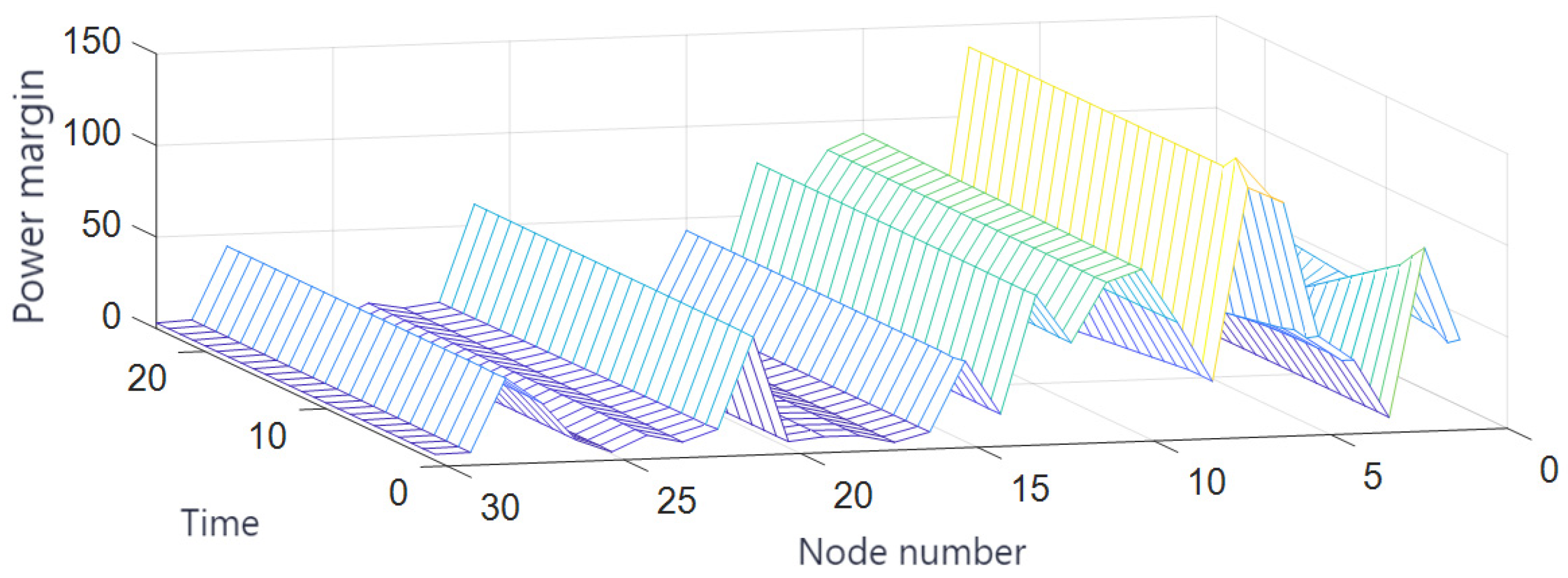
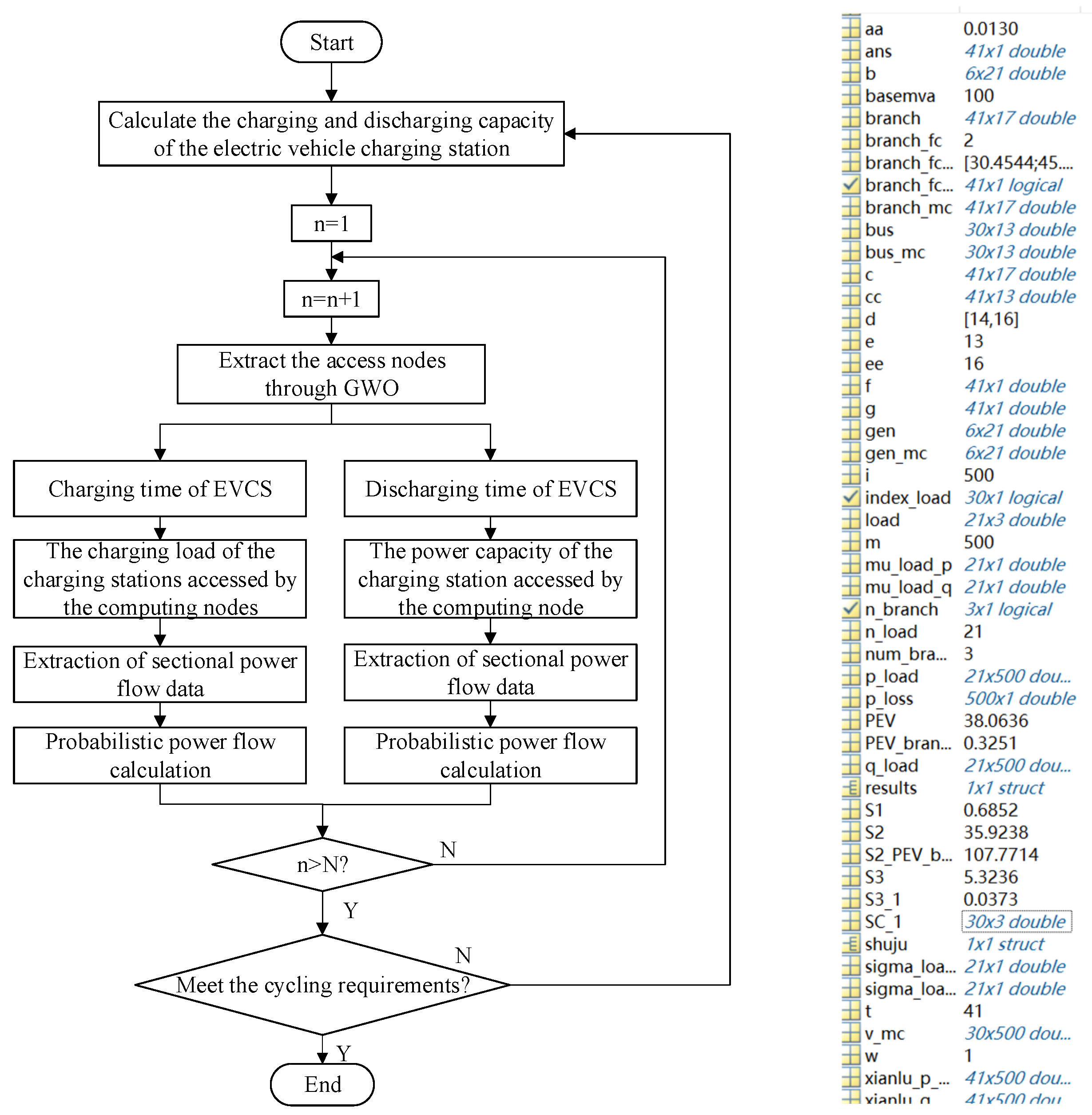
4. Dynamic Data Extraction of the Distribution Network Based on Time-Segmented Power Flow

Against the backdrop of the new energy revolution, along with the addition of various variables represented by EVs, it has become gradually more difficult to meet the actual demands of deterministic power flow [18]. Hence, in this paper, the Monte Carlo simulation method is employed. Through MATLAB, the fluctuation of the random variable is set at 30%. A large number of samplings of the random variable are conducted, and the sampling results are substituted into the power flow calculation, thereby obtaining the power flow data after considering the load fluctuation.

According to the multi-objective optimization scheme proposed in Section 2, it is necessary to extract the power flow data of the distribution network after accessing the EVCS. In real life, the power flow data of the distribution network are constantly changing. If calculated based on the traditional deterministic power flow, there will be a certain deviation from the actual result. In this paper, the dynamic data of the distribution network is extracted by solving the tidal current in various time periods, and the results are presented in Figure 4 as follows:

Figure 4. Data extraction of segmented power flow.

Take area A in the above figure as an example, namely, where the EVCS charges the EV. At this juncture, the EVCS is connected to the distribution network as a load. Through the Newton–Leibniz formula, supposing that the distance between each dotted line is ΔX, the more the area A is divided by the dotted lines, the smaller ΔX becomes. When the number of divisions approaches the limit, the curve value corresponding to ΔX at this time can be approximately regarded as invariant.

The actual power flow is subject to dynamic variations. Nevertheless, when the time is narrowed to a specific value, the power flow data at that time can be approximately treated as a deterministic power flow. In this paper, the charging and discharging time of the EVCS is segmented at one-minute intervals. At this juncture, extracting the dynamic data of the distribution network can significantly reduce the error. Based on the segmentation results, there are 60 sets of power flow data within one hour. Integrating and averaging all the data can yield a set of power flow data considering load fluctuations. A reasonable EVCS location optimization scheme can be optimized via the gray wolf algorithm.

However, conducting only one segmentation might result in certain deviations. Hence, through a large number of cycles, the most reasonable optimization scheme is selected from the data after the cycles. This scheme can greatly minimize the error and be closer to the actual situation. The probabilistic power flow calculation of the distribution network with EVCS and taking into account its charging and discharging capacity is presented in Figure 5.

Figure 5. Flow chart of power flow calculation of distribution network with EVs.

5. Solution to Optimization Scheme of Electric Vehicle Charging Stations Based on Gray Wolf Algorithm

5.1. The Classification of Wolves Within a Group

In GWO, each solution is associated with a wolf. The leading wolf α represents the current optimal solution, while the wolves β and δ representing the suboptimal solutions, and the remaining solutions are the ω wolves. α, β, and δ jointly determine the search direction [19].

5.2. Surrounding the Quarry

In the wolf pack, the positions of α, β, and δ have an impact on the subsequent movement of each wolf. In the GWO algorithm, this process is presented as follows:

$$D=\left|C{X}_P(u)-X(u)\right|$$

(34)

$$X(u+1)=X_P(u)-AD$$

(35)

where A and C represent coefficient vectors; X_p(u) indicates the orientation of α, β, and δ; and X(u) and X(u + 1), respectively, denote the orientations of any solution before and after being influenced by X_p(u) [20].

5.3. Aggressive Behavior

In the GWO algorithm, the attacking direction can be represented as

$$X(u+1)={\displaystyle \frac{X_1+X_2+X_3}{3}}$$

(36)

where X₁, X₂, and X₃ represent the moving directions of each wolf and are, respectively, influenced by α, β, and δ, and the three jointly determine the new directions of each wolf [21].

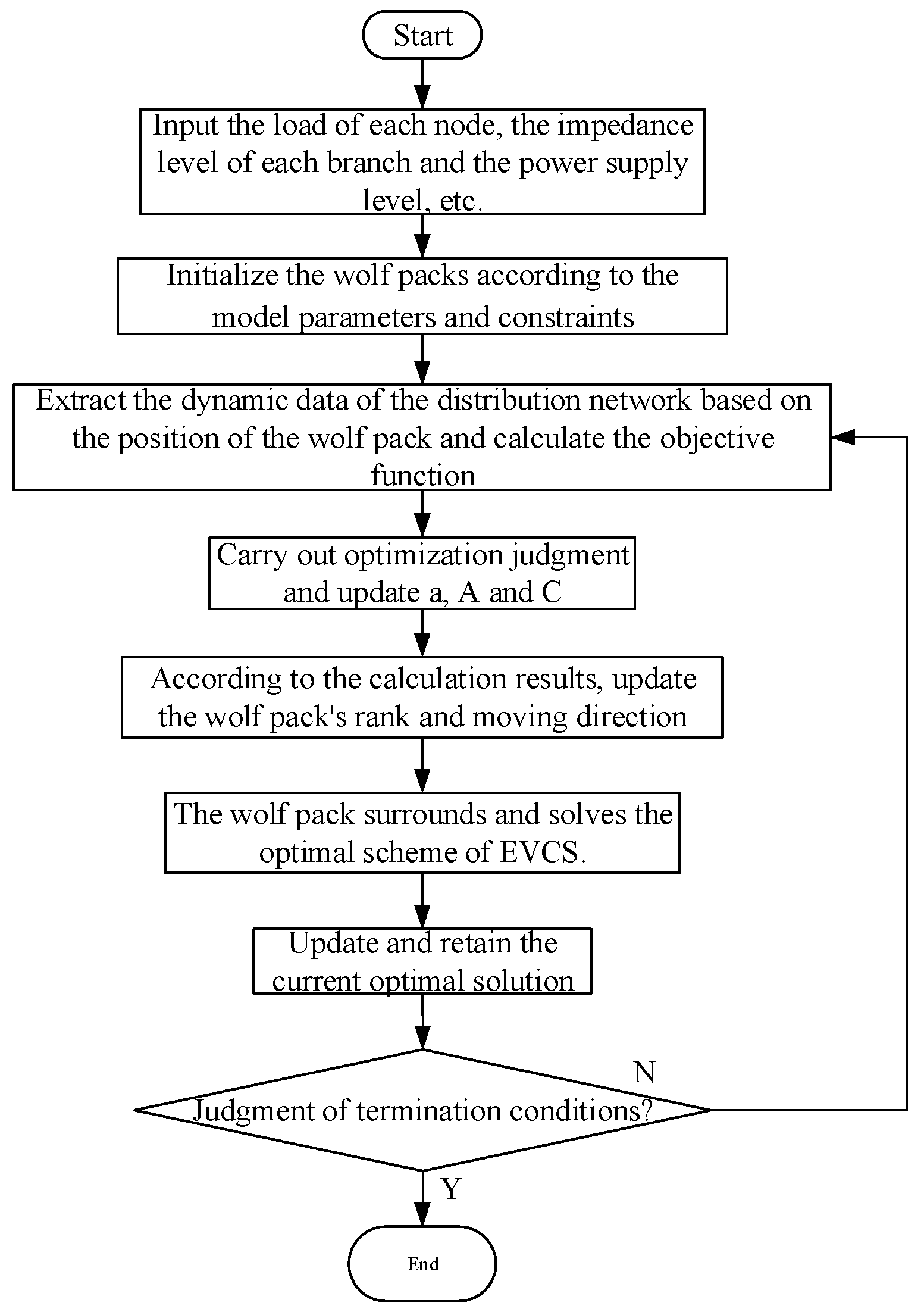
5.4. Solution of the Optimization Scheme for Electric Vehicle Charging Stations Based on the Gray Wolf Algorithm

Once the EVCS is connected to the distribution network, the influence of the EVCS on the distribution network subsequent to the connection is minimized by optimizing the access location of the EVCS. In accordance with the scheme proposed herein, the location planning of M EVCSs in a road–electricity coupling network consisting of N nodes is conducted. The constraint conditions are intricate and the computational volume is substantial. Hence, this paper employs the gray wolf algorithm to solve the proposed scheme presented in this paper. The solution steps are as follows [22,23,24,25]:

Step 1: Input the load of each node, the impedance level of each branch, the power supply level, and so on.

Step 2: Initialize the capacity of the electric vehicle charging station and the positions of each wolf pack in accordance with the model parameters and constraint conditions, namely, the initial positions of M EVCSs.

Step 3: Based on the positions of the initialized wolf packs, calculate the value of the objective function by means of the dynamic data extraction method of the distribution network proposed in Section 3.

Step 4: Conduct optimization judgment based on the computed results. The optimal solution is regarded as the leading wolf. Update a and the synergy coefficient vector A, and concurrently update the random weight C of the current solution’s influence on the prey.

Step 5: Based on the calculation and comparison outcomes of the initial position of the EVCS, update the classification of the wolf pack and the moving direction of each wolf pack, and determine the new position of the wolf pack.

Step 6: Approach and encircle the optimal deployment points of EVCSs.

Step 7: According to Step 2, during the encircling process, solve the result of each hunting, retain the optimal solution, and determine whether the stop condition is fulfilled. If it is fulfilled, the hunting terminates; otherwise, return to Step 2 and continue the solution.

Step 8: Until the optimal solution is obtained or the maximum convergence number is reached, output the optimal deployment planning scheme of EVCSs.

The specific algorithm flow is presented in Figure 6 below.

Figure 6. Model calculation flow chart.

6. Simulation Analysis

To validate the efficacy of the proposed scheme, in this paper, the working conditions of an EVCS on a typical working day are chosen for simulation. The EVCS encompasses charging interfaces for all types of EVs. The EV charging simulation period ranges from 00:00 to 24:00, with a time interval of ten minutes, and the extraction time of segmented power flow data is from 00:00 to 24:00, with a time interval of one minute. The battery capacity of various EVs is presented in Table 3 as follows:

Table 3. Table showing the battery capacity of various EVs.

EV Types	Capacity Size
Electric bus	55 kWh
Electric taxi	45 kWh
Electric official cars and special vehicles	35 kWh
Electric private car	35 kWh

The specific weights of each element calculated based on the Analytic Hierarchy Process are presented in Table 4 as follows:

Table 4. The weight of each element in the objective function.

Weights	Value	Weights	Value
K1	0.217	K7	0.217
K2	0.217	K8	0.217
K3	0.217	K9	0.166
K4	0.166	K10	0.183
K5	0.183	K11	0.586
K6	0.217	K12	0.414

For the sake of facilitating our research, the following assumptions are made prior to the calculation in this paper:

(1)

The number of EVs has attained a certain scale, and the EVCS can perpetually remain in normal operation.

(2)

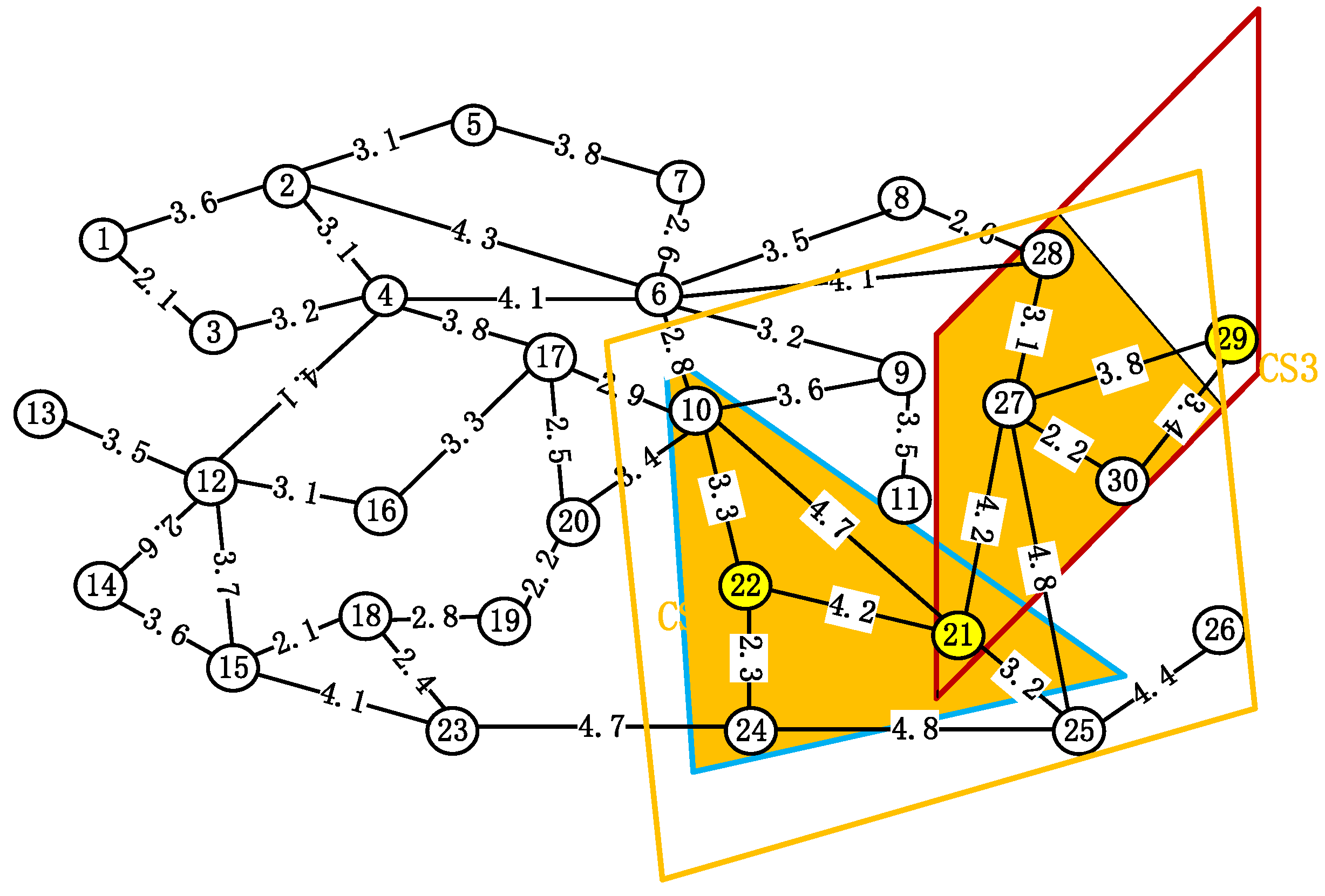
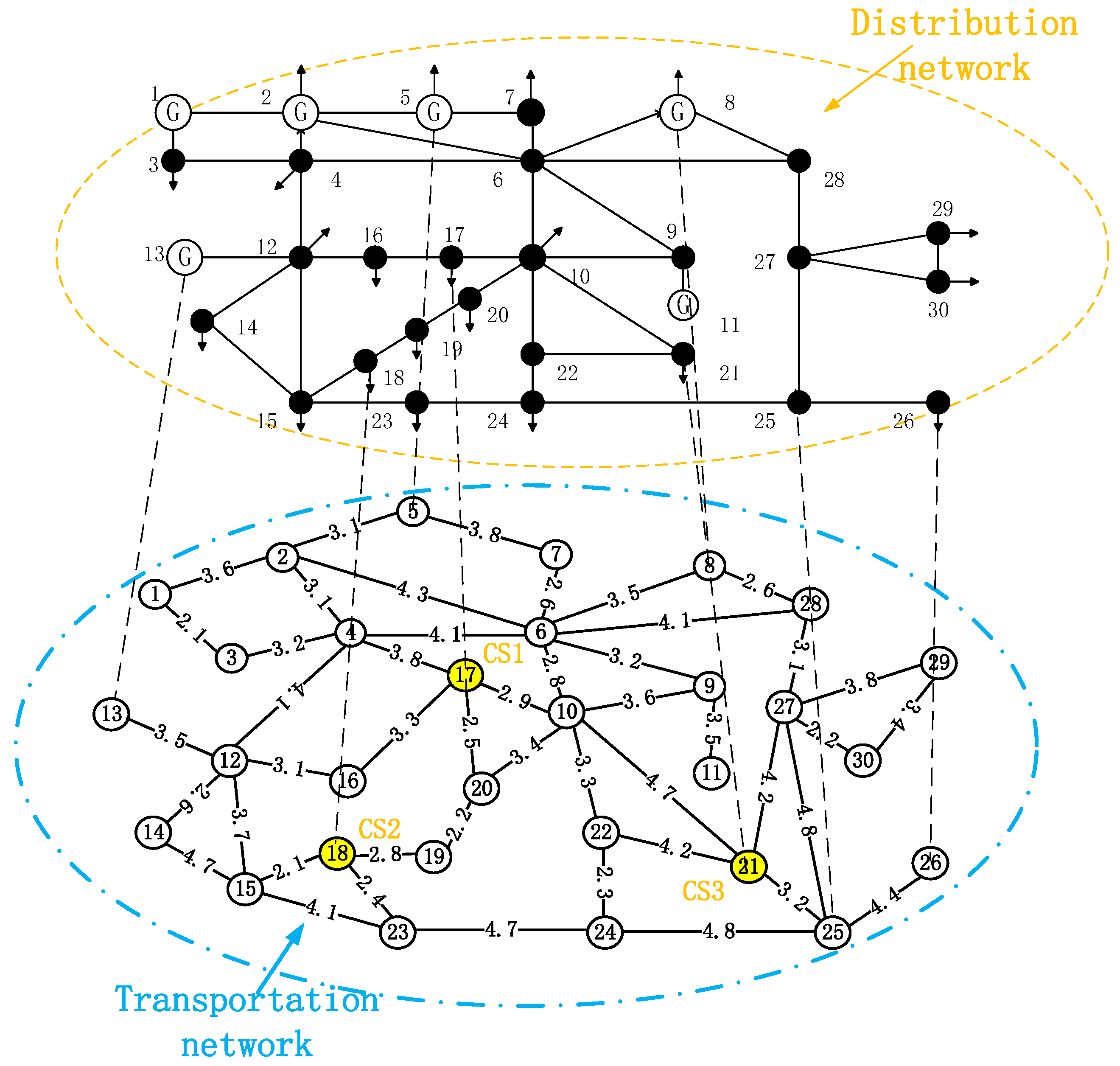
The IEEE-30 node standard example is adopted herein, and the data are in accordance with the example.

(3)

Based on the simulation results of the EV daily load curve, the capacity of the EVCS is 1.3 MW; the backup energy storage power supply is 1.3 MW; for the charging time and the discharging time, the output is 1.3 MW; the expected SOC is 1; and the charging pile efficiency η is taken as 0.95.

(4)

The charging process in this paper is simplified to the constant power characteristic, and the conventional charging power is taken as 3 KW and the fast charging power is taken as 48 KW.

This paper employs the coupling framework of the IEEE 30 distribution network and 30 road network nodes for simulation analysis [26,27]. The corresponding coupling framework of the distribution network and the transportation network is depicted in Figure 7. The unit distance between nodes in the figure is 1 KM. The corresponding charging station locations are indicated by yellow nodes, and in the subsequent figure, the number of charging stations is taken as M = 3, for instance. The nodes connected by the dotted lines in the figure are defined as the coupling nodes of the power grid and the transportation network.

Figure 7. Distribution network–transportation network coupling framework.

The weight of the influence factors of each node can be seen in Table A5.

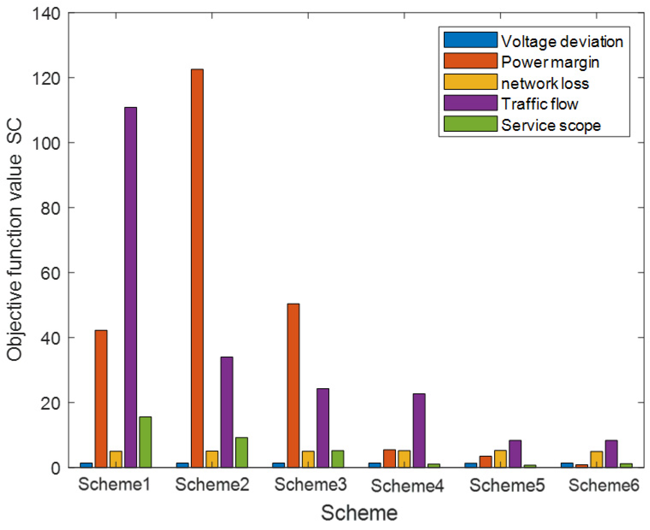
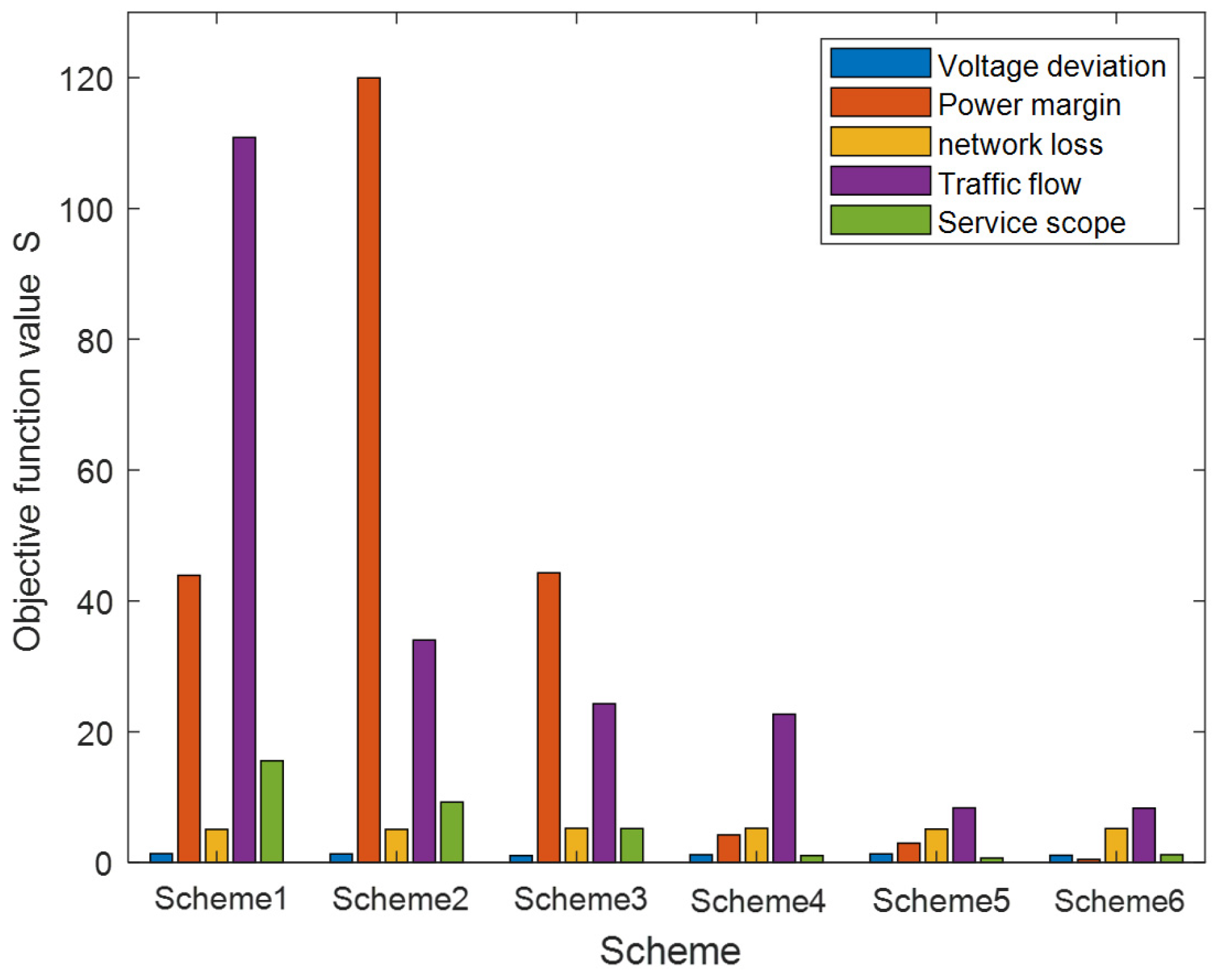
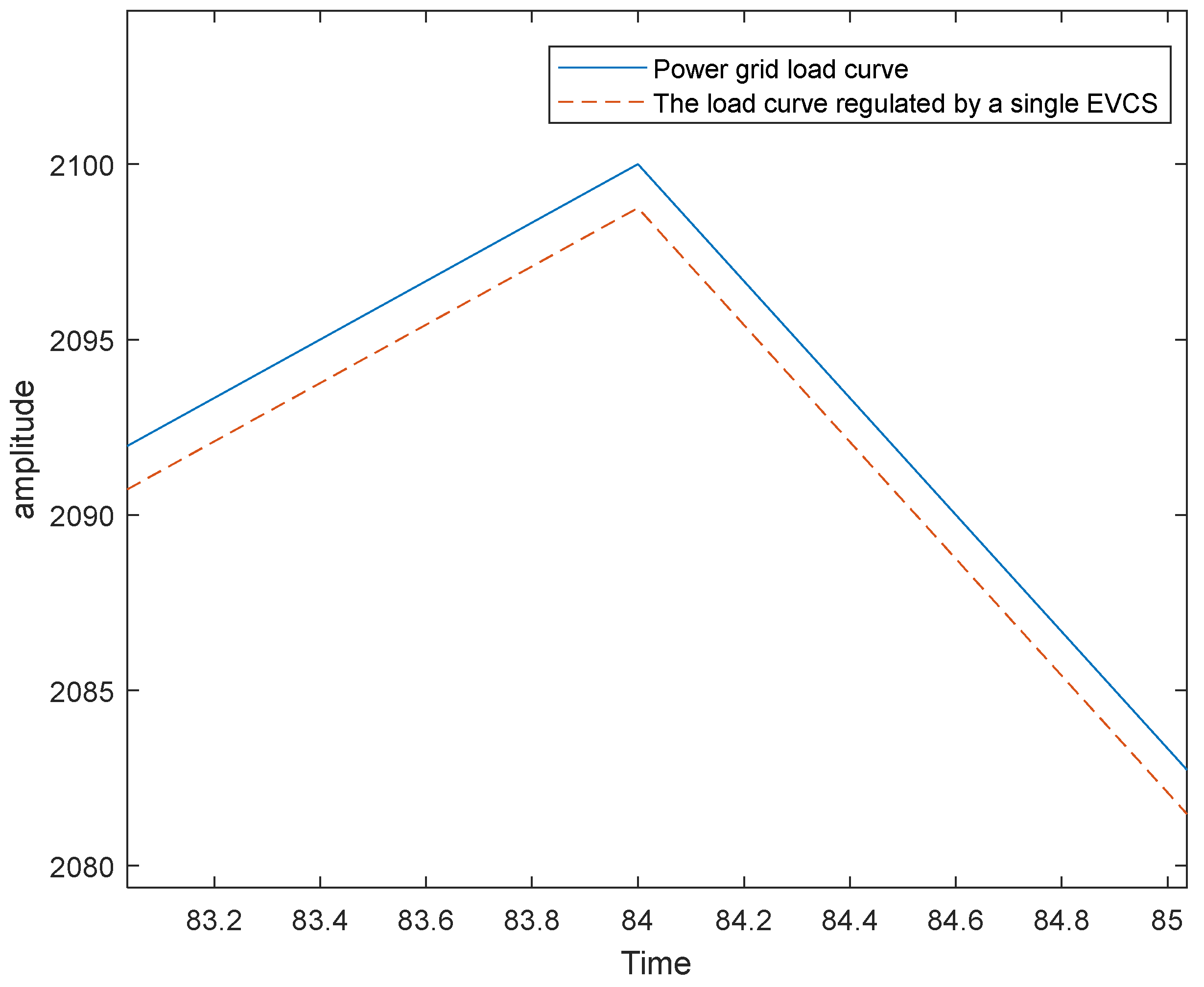
6.1. Planning Scheme for Single-Charge Station

In the IEEE-30 node standard example, nodes 1, 2, 5, 8, 11, and 13 are reference nodes and PV nodes, which typically represent power plants and power stations. Consequently, they are not regarded as planning nodes for EVCSs. When M = 1, six schemes are devised for simulation verification. Scheme 6 is the optimal one identified by GWO. The various schemes are presented in Table 5 as follows:

Table 5. Single-seat charging station plan table.

Scheme	Nodes	Scheme	Nodes
Scheme 1	7	Scheme 4	24
Scheme 2	12	Scheme 5	30
Scheme 3	19	Scheme 6	17

When the single EVCS is connected to the road-electricity coupling network in accordance with the planning scheme proposed in this paper, the traffic flow and service scope of each scheme are presented in Table 6 as follows:

Table 6. The factor table of the road network for the single-seat EVCS.

Scheme	Node Traffic Flow	S5 objective Function Value	Scope of Service
Option 1	110.875	10.564	3 nodes
Scheme 2	34.001	8.231	4 nodes
Scheme 3	24.298	5.215	6 nodes
Scheme 4	22.700	1.061	10 nodes
Scheme 5	8.3467	4.103	7 nodes
Scheme 6	8.3328	3.213	9 nodes

It can be discerned from Section 3.6 that the establishment of the objective function value for traffic flow is to fulfill the optimization of the GWO algorithm and is configured in the reciprocal form. That is, the smaller the objective function value, the larger the traffic flow at this node. Hence, it can be observed from the aforementioned table that the traffic flow of Scheme 6 surpasses that of the other schemes. The number of service range nodes of Scheme 4 is set to 10 service nodes due to the constraint of Equation (31). The node diagrams of the service scope of Schemes 1–5 can be seen in Figure A1, Figure A2, Figure A3, Figure A4 and Figure A5. Moreover, the optimization data of the objective functions SC and SF are acquired through GWO. The data comparison of each scheme is depicted in Figure A6 and Figure A7. By combining the values of the objective functions SC and SF, when a single EVCS is connected to the distribution network, the optimization data of the six schemes are obtained, and the corresponding optimization results are shown in Figure 8:

Figure 8. Comparison of objective function S schemes.

It can be observed from the aforementioned figure that the objective function values of Schemes 5 and 6 are conspicuously superior to those of the other four schemes, and we can also see the optimization process and efficacy of GWO. In combination with Table 6 and the data comparison, it can be ascertained that the objective function value corresponding to Scheme 6 is the optimum. Hence, the index corresponding to the single EVCS connected to Node 17 will be more favorable. Figure A8 and Figure A9 present the power margin of each node within 24 h when the EVCS is connected to the distribution network as a load and power source.

The service scope of Scheme 6 is presented in Figure 9 as follows:

Figure 9. The service area of the charging station in Scheme 6 for a single-seat EVCS.

From the aforementioned simulation outcomes, it can be discerned that in accordance with the optimization scheme put forward in this paper, when a solitary EVCS is connected to the road–electricity coupling network, it is capable of maximizing the service scope while fulfilling the charging requirements, and can effectively mitigate the impact of EVCSS on the power grid and stabilize the operation of the power grid.

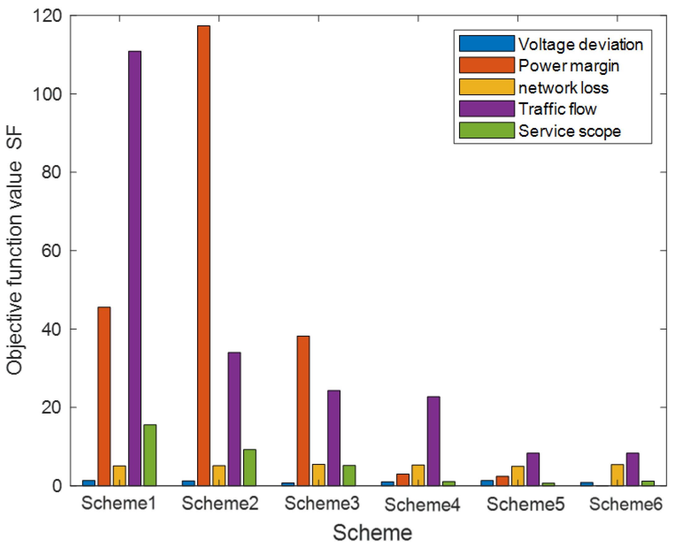
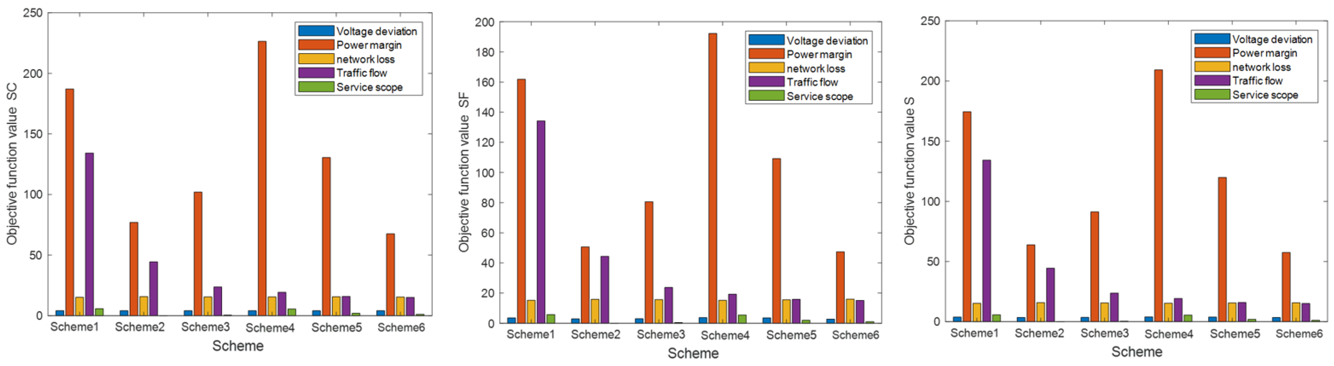
6.2. Schemes for Planning Multiple Charging Stations

When M equals 3, the location planning of the road–electricity coupling network is conducted in accordance with the scheme proposed in this paper. As stated in Section 5.1, six schemes are set for simulation verification. The specific plan is presented in Table 7 as follows:

Table 7. Multi-seat charging station plan table.

Scheme	Nodes
Scheme 1	17, 7, 28
Scheme 2	22, 21, 29
Scheme 3	22, 13, 23
Scheme 4	20, 7, 13
Scheme 5	30, 15, 11
Scheme 6	17, 21, 18

Combined with the transportation network and solved by GWO, when EVCS is connected in accordance with the above schemes, the traffic flow and service scope of each scheme are presented in Table 8:

Table 8. The factor tables of the road networks of multiple charging stations.

Scheme	Node Traffic Flow	S5 Objective Function Value			Scope of Service (Number of Nodes)
		S5.1	S5.2	S5.3
Scheme 1	134.220	4.165	10.242	4.043	7	3	7
Option 2	44.361	10.242	1.940	7.075	3	10	4
Option 3	23.742	20.537	2.250	14.554	2	10	3
Option 4	19.286	3.970	1.940	8.085	7	10	4
Scheme 5	15.914	4.063	3.464	8.768	7	9	3
Scheme 6	15.093	4.043	3.995	3.995	8	8	8

As depicted in the aforementioned table, the traffic flow at the node where the EVCS is situated in Scheme 6 is superior to that in the other schemes. Owing to the constraint of Formula (31) in Schemes 3–5, the minimum is Node 2 and the maximum is Node 10. The node diagrams of the service scope of specific Schemes 1–5 can be found in Figure A10, Figure A11, Figure A12, Figure A13 and Figure A14

When the EVCS is connected to the road–electricity coupling network as a load, the optimized data of each scheme are compared as depicted in the following figure:

As depicted in the figure above, the objective function of Scheme 6 is conspicuously superior to that of the other five schemes. Nevertheless, the planning scheme proposed in this paper has to take into account not only the load characteristics of the EVCS but also the energy storage characteristics of the EVCS. The optimization data of the objective function SF of each scheme when multiple EVCSs are connected to the road–electricity coupling network as power sources are presented in Figure 10. When the EVCS is connected to the coupling network as a power source, each objective function of Scheme 6 is also the optimum. By combining the values of the objective functions SC and SF, when multiple EVCS were connected to the road–electricity coupling network, the optimization data of the six schemes were obtained, and the corresponding optimization results are presented in Figure 10.

Figure 10. Diagrams comparing the objective function schemes.

Combining Table 8 and the comparison among the abovementioned schemes, it can be ascertained that the objective function value corresponding to Scheme 6 is the most optimal. When EVCS functions as a load, the voltage deviations of each node within 24 h are presented in Figure 11, and the power margin is depicted in Figure A15:

Figure 11. Voltage deviation of each node at the time of charging.

The power margin of each node when the EVCS is connected to the distribution network as a power source is presented in Figure A16. The service scope of Scheme 6 is presented in Figure 12 as follows:

Figure 12. The plan regarding multiple charging stations encompasses the service scope of 6 charging stations.

The information table of the service scope of each plan is presented in Table 9 as follows:

Table 9. Service scope information table.

Scheme	Scope Coverage	Number of Nodes with No Coverage	Coincidence Ratio	Percentage of No Overlay
Scheme 1	50.00%	15	16.67%	50.00%
Option 2	36.67%	19	23.33%	63.33%
Option 3	50.00%	15	10.00%	50.00%
Option 4	73.33%	8	6.67%	26.67%
Scheme 5	73.33%	8	0%	26.67%
Scheme 6	83.33%	5	13.33%	16.67%

It can be discerned from the aforementioned table that Scheme 6 possesses the widest coverage range. Within the entire road–electricity coupling network, Scheme 6 has the fewest uncovered nodes. Although its service area overlap rate is marginally higher than those of Schemes 3–5, by comparing Figure A10, Figure A11, Figure A12, Figure A13, Figure A14 and Figure 12, the number of uncovered nodes in Scheme 3 is too large to satisfy the requirements of EV users. Although Schemes 4 and 5 have an edge in the service area overlap degree, the locations of EVCSs in them are inferior to that of Scheme 6. The nodes where EVCSs are located in Scheme 4 are slightly inclined towards the front section of the road–electricity coupling network, and the nodes where EVCSs are located in Scheme 5 are more inclined towards the end of the network. The location in Scheme 6 can optimally meet the needs of EV users. To conclude, Scheme 6 is the most optimal scheme compared to the other schemes.

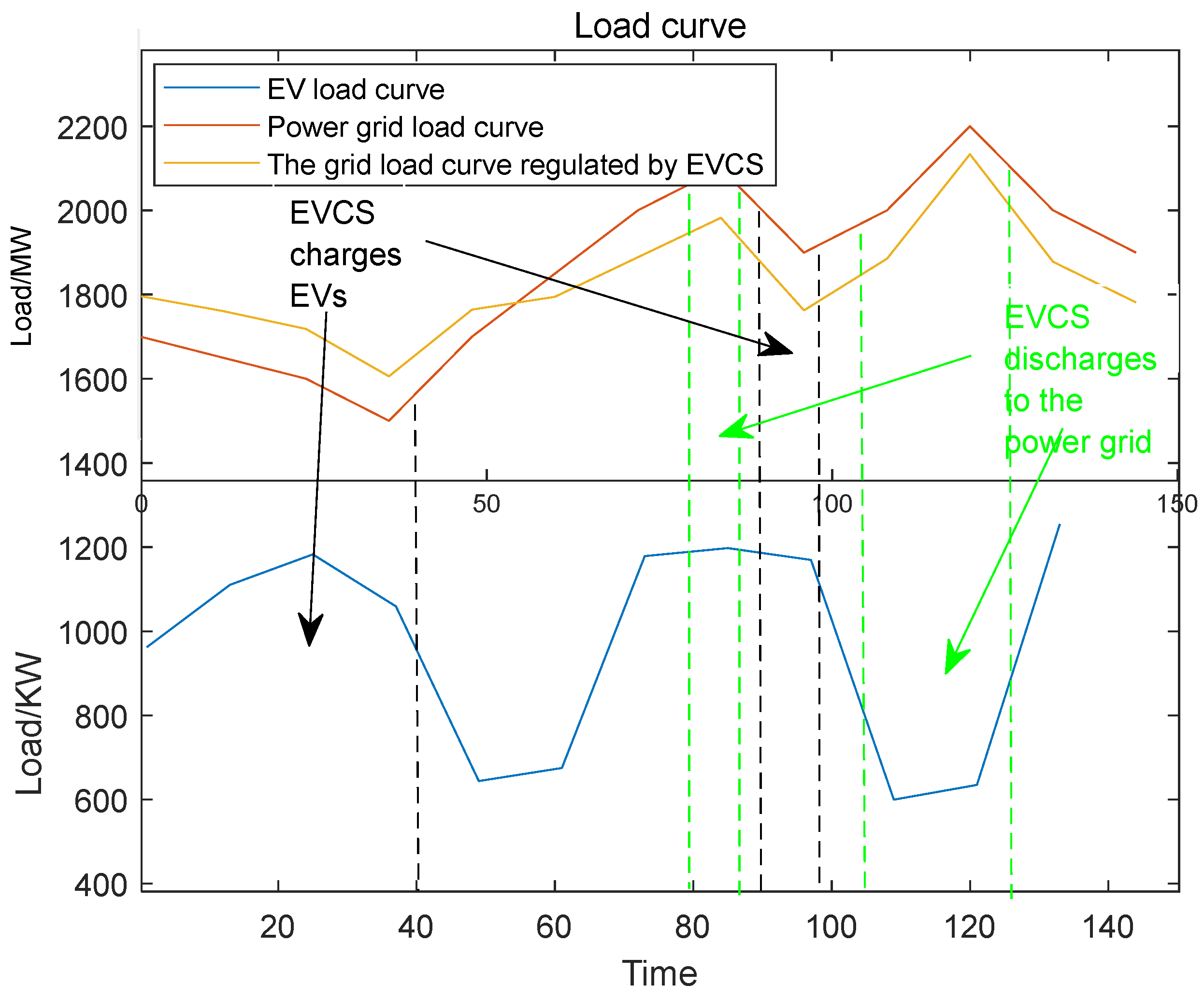
6.3. Simulation of Regulatory Benefits Based on Peak Shaving and Valley Filling

After the EVCS is connected to the road–electricity coupling network in accordance with the scheme proposed in this paper, it can effectively reduce the peak load and fill the trough load. The trough of the daily load curve of the power grid after regulation with a single EVCS is presented in Figure 13 as follows:

Figure 13. Single EVCS peak-clipping and valley-filling map (wave valley).

The peak of the daily load curve of the power grid after the regulation with the participation of a single EVCS is depicted in Figure 14:

Figure 14. Single EVCS peak-clipping and valley-filling diagram (wave crest).

The above figure depicts the partial daily load curve of the power grid. Once the EVCSs adjusted the daily load curve of the power grid in accordance with the scheme proposed herein, an evident trend of peak shaving and valley filling could be witnessed. Owing to capacity constraints, the regulation of the distribution network load curve by the EVCSs in this paper is not substantial. Nevertheless, based on the optimization scheme put forward in this paper, the daily load curve of the power grid after the participation of the EVCS group in the regulation when the number of EVCSs attains a certain scale is presented in Figure 15:

Figure 15. The daily load curve of the power grid after the EVCS participates in regulation.

As depicted in the above figure, the fluctuation of the daily load curve is conspicuously suppressed. Hence, it can be observed that when the EVCS operates optimally in accordance with the charging and discharging scheme proposed herein, it can efficaciously regulate the daily load curve of the power grid, fulfill the goal of peak shaving and valley filling, and enhance the reliability of the power supply. This also fully substantiates the effectiveness of the EVCS planning scheme investigated in this paper.

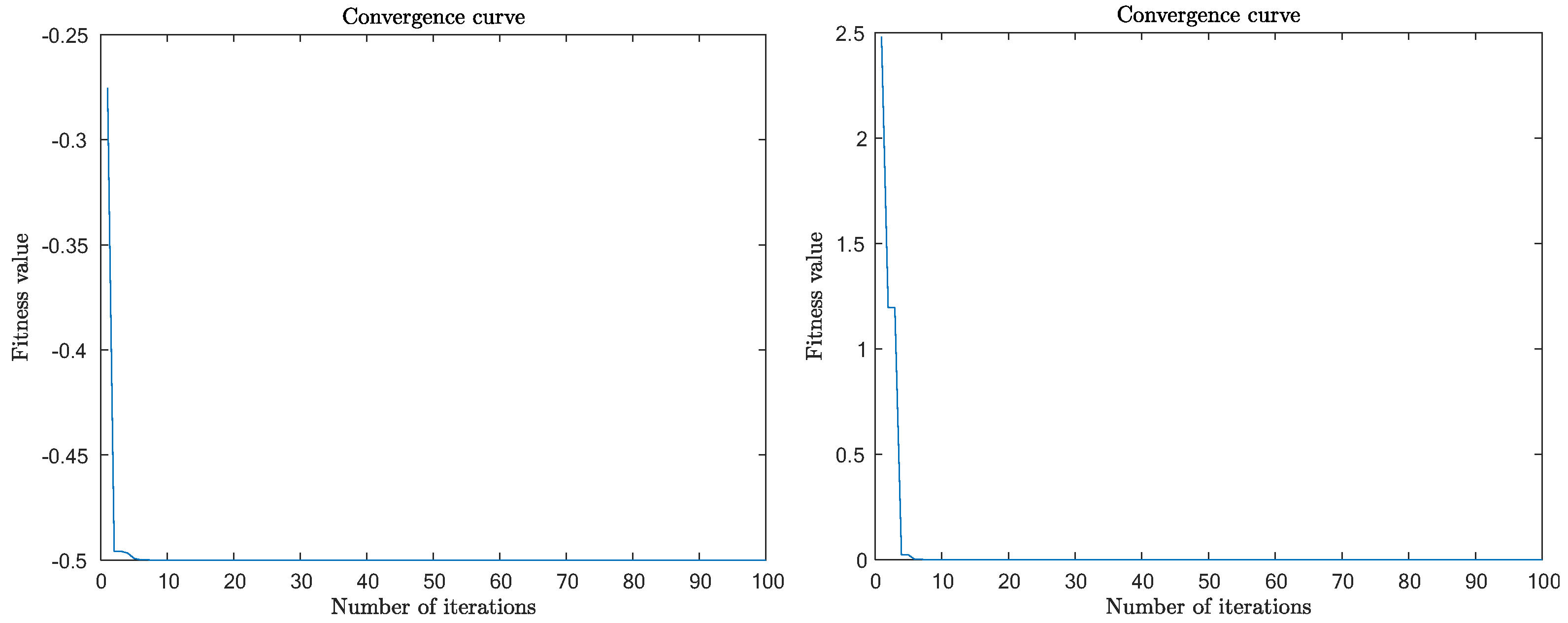
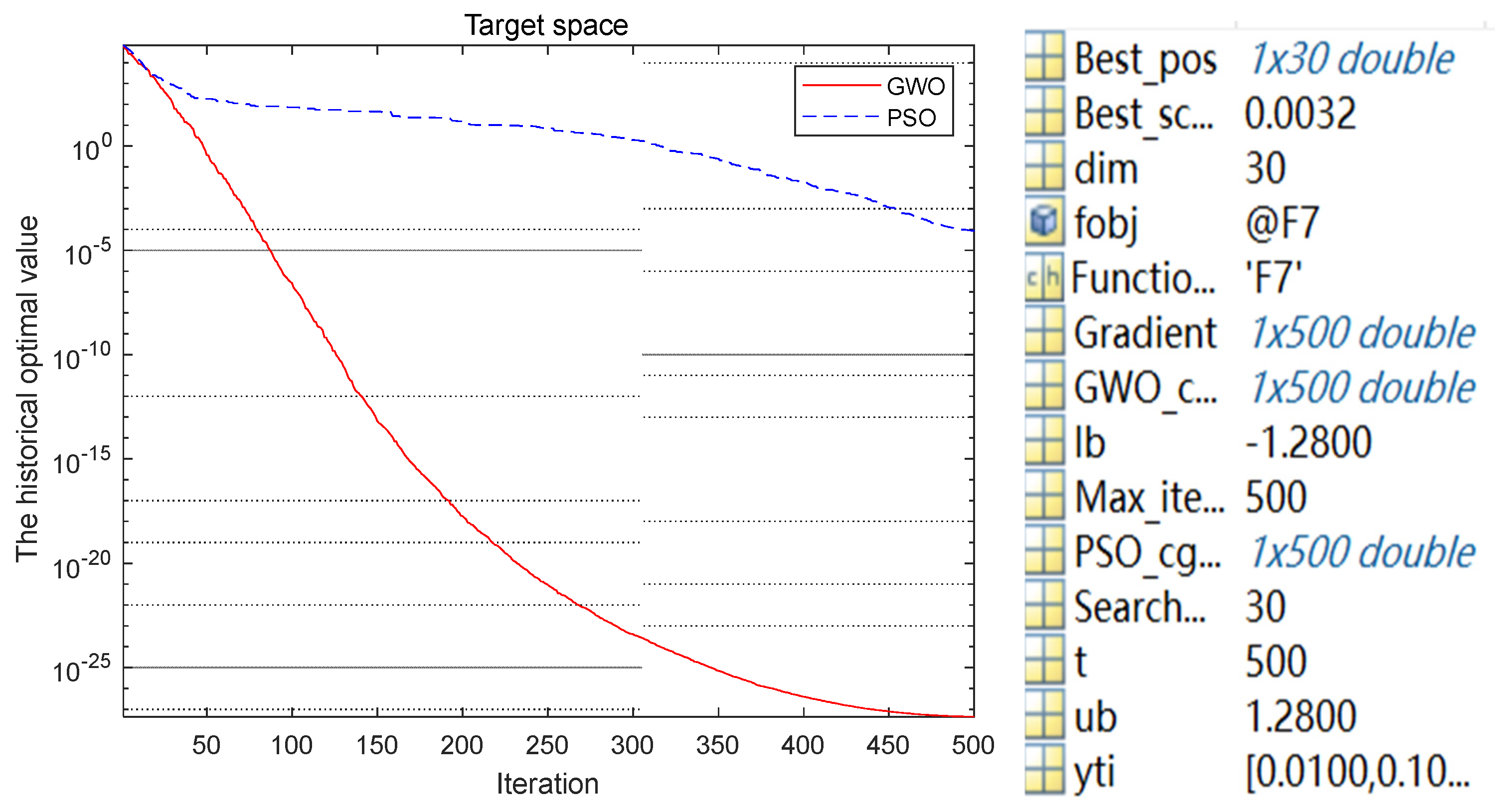
6.4. Comparison of Optimization Algorithms: A Comprehensive Study

This paper performs a sensitivity analysis and a robustness test on the model, taking into account the impact of random fluctuations of parameters on the solution. Figure 16 presents the robustness simulation diagram of the model.

Figure 16. Robustness simulation diagram.

The GWO algorithm is chosen as the heuristic approach for the location optimization issue of electric vehicle charging stations because of its strengths in global search capability and convergence speed. Compared with the gradient algorithm, the GWO algorithm holds more advantages when dealing with such complex optimization problems. Table 10 presents the comparison of algorithm characteristics.

Table 10. Algorithm comparison information table.

Characteristics	GWO	PSO	Gradient Algorithm
Heuristic type	Swarm intelligence	Swarm intelligence	Gradient-based
Speed of convergence	Fast	Faster	Depends on function properties
Global search capability	Strong	Strong	Weak
Parameter quantity	Less	Less	Less
Applicability	Complex optimization problems	Extensive	Simple optimization problems
Sensitivity to initial solutions	Low	Low	High

This paper conducts a comparison between the optimization processes and results of the Gray Wolf Optimizer (GWO) and particle swarm optimization (PSO), and the comparison outcomes are presented in Figure 17:

Figure 17. Comparison of optimization process between GWO and PSO.

As depicted in the figure above, the optimization processes of GWO and PSO for multiple objective functions are compared. Within the 500-iteration range, GWO attains the optimal value earlier than PSO and reaches the convergence condition. Concerning the location optimization problem of electric vehicle charging stations in this paper, the comparison results of the two algorithms are presented in Table 11 as follows:

Table 11. Comparison table of solution plans.

Algorithm	Optimization Scheme (X1, X2, X3)	Composite Indicators	Grid Indicators (S1, S2, S3)	Road Network Indicators (S4, S5)	Convergence (500 Times)
GWO	(17, 21, 18)	18.532	(3.41, 57.48, 15.66)	(15.09, 1.05)	Yes
PSO	(19, 16, 23)	26.92	(3.53, 91.27, 15.62)	(23.74, 0.44)	No

Compared with the PSO algorithm in the location optimization of electric vehicle charging stations, GWO, using coefficient vector A in Formula (35) to balance the ability of global search and local search, acquires the smallest comprehensive index. Both GWO’s power grid index and road network index are superior to the results of the PSO algorithm, and it outperforms the PSO algorithm in terms of convergence speed and solution accuracy, reflecting the reliability of the optimal location planning scheme of EVCS based on GWO in this paper.

7. Conclusions

This paper examines the complementary features of the load curves of the power grid and EVCSs and investigates the influence of EVCSs, both as a load and a power source accessing the distribution network, on the power grid and transportation network. By optimizing the location of EVCSs, the regulation benefit based on peak shaving and valley filling is optimal after EVCSs are connected to the road–electricity coupling network, and the power quality of the distribution network, traffic flow, and service scope of EVCSs reach their best state. Meanwhile, the EVCS layout planning scheme proposed in this study enables the number of charging stations to be preset and optimized on this basis, enhancing the adaptability and practicability of the scheme and better meeting actual demands.

This paper thoroughly discusses the dual role of EVCSs as a power source and load in the power grid and their impact, and makes an initial plan for their internal backup energy storage power source. However, energy storage can also achieve peak load transfer through energy transfer, frequency regulation, etc. Based on this, future research can further deepen the study of the energy storage characteristics of EVCSs, including their energy storage capacity and response speed, and refine the charging and discharging strategy proposed in this study to optimize the charging and discharging scheme of EVCSs.

References

- Tian, M.; Tang, B.; Yang, X.; Xia, X. Planning of electric vehicle charging station comprehensively considering the charging demand and the acceptance capacity of the distribution network. Power Syst. Technol. 2021, 45, 498–509. [Google Scholar]
- Clement-Nyns, K.; Haesen, E.; Driesen, J. The impact of charging plug-in hybrid electric vehicles on a residential distribution grid. IEEE Trans. Power Syst. 2018, 25, 371–380. [Google Scholar] [CrossRef]
- Lu, S.; Ying, L.; Wang, X.; Li, W. Load forecasting and optimal dispatching of electric vehicle fast charging stations based on user travel simulation. Electr. Power Constr. 2020, 41, 38–48. [Google Scholar]
- Pal, A.; Bhattacharya, A.; Chakraborty, K. Allocation of electric vehicle charging station considering uncertainties. Sustain. Energy Grids Netw. 2021, 24, 38–48. [Google Scholar] [CrossRef]
- Cheng, S.; Chen, Z.; Xu, K.; Kang, Z.; Wei, Z. Orderly charging and discharging method of electric vehicles based on cooperative game and dynamic time-of-use electricity price. Power Syst. Prot. Control 2020, 48, 15–21. [Google Scholar]
- Ge, S.; Shen, K.; Liu, H. Urban fast charging network planning considering network transfer performance. Power Syst. Technol. 2020, 63, 1–13. [Google Scholar]
- Wu, Y.; Wang, Y.; Zhang, Y.; Xue, H.; Mi, Y. Location and capacity method of electric vehicle charging station based on improved immune clonal selection algorithm. Autom. Electr. Power Syst. 2021, 45, 1–11. [Google Scholar]
- Deb, S.; Gao, X.-Z.; Tammi, K.; Kalita, K.; Mahanta, P. A Novel Chicken Swarm and Teaching Learning based Algorithm for Electric Vehicle Charging Station Placement Problem. Energy 2020, 15, 12–18. [Google Scholar] [CrossRef]
- Yan, Q.; Liu, H.; Han, N.; Songsong, C.; Dongming, Y. An optimization method for the location and capacity of charging stations taking into account the temporal and spatial distribution of electric vehicles. Proc. Chin. Electr. Eng. 2021, 41, 1–14. [Google Scholar]
- Cheng, S.; Zhao, M.; Wei, Z. Optimal scheduling of electric vehicle charging and discharging with dynamic electricity prices. J. Electr. Power Syst. Autom. 2020, 31, 1–7. [Google Scholar]
- Zhang, J. Research on orderly charging strategy and charging facility planning of electric vehicles. Ph.D. Thesis, Taiyuan University of Technology, Taiyuan, China, 2018; pp. 8–11. [Google Scholar]
- Li, C.; Dong, Z.; Li, J.; Zhang, H.; Jin, Q.; Qian, K. Distributed energy storage cluster voltage regulation control strategy for distribution network. Autom. Electr. Power Syst. 2021, 45, 133–141. [Google Scholar]
- Cheng, S.; Zhao, M.; Wei, Z. Optimal Scheduling of Electric Vehicle Charging and Discharging Considering Dynamic Electricity Price. Proc. CSU-EPSA 2021, 33, 31–36+42. [Google Scholar]
- Cavus, M.; Allahham, A. Enhanced Microgrid Control through Genetic Predictive Control: Integrating Genetic Algorithms with Model Predictive Control for Improved Non-Linearity and Non-Convexity Handling. Energies 2024, 33, 1–20. [Google Scholar] [CrossRef]
- Shi, J.; Bao, Y.; Chen, Z.; Jiang, Z.; Zhang, W. A Robust Optimal Configuration Method for Charging Station Energy Storage Considering the Uncertainty of Charging Load. Autom. Electr. Power Syst. 2021, 10, 1–16. [Google Scholar]
- Ni, S.; Cui, C.; Yang, N.; Chen, H.; Xi, P.; Li, Z. Multi-time scale online reactive power optimization of distribution network based on deep reinforcement learning. Autom. Electr. Power Syst. 2021, 45, 77–85. [Google Scholar]
- Nezamoddini, N.; Wang, Y. Risk management and participation planning of electric vehicles in smart grids for demand re-sponse. Energy 2016, 20, 22–28. [Google Scholar]
- Wang, X. Research on Reactive Power Optimization of Multi-Scenario Distribution Network with Wind Turbines. Ph.D. Thesis, Xi’an University of Technology, Xi’an, China, 2019; pp. 28–31. [Google Scholar]
- Amin, Y.; Abbasian, J.M.; Ma, J. Electric vehicle charging station location determination with consideration of routing selection policies and driver’s risk preference. Comput. Ind. Eng. 2021, 69, 162–169. [Google Scholar]
- Lee, S.; Choi, D.H. Dynamic pricing and energy management for profit maximization in multiple smart electric vehicle charging stations: A privacy-preserving deep reinforcement learning approach. Appl. Energy 2021, 42, 304–315. [Google Scholar] [CrossRef]
- Ding, Y.; Yao, X.; Ge, X.; Bingxue, Y.; Jiawei, L.; Yu, S. Calculation and analysis of DC pole-tower gap operating impulse voltage based on Adaboost-SVR prediction. Proc. Chin. Soc. Electr. Eng. 2021, 41, 1–10. [Google Scholar]
- Pan, Z.; Zhang, X.; Yu, T.; Wang, D. Hierarchical real-time optimal scheduling of large-scale electric vehicle clusters. Autom. Electr. Power Syst. 2017, 41, 96–104. [Google Scholar]
- Mirjalili, S.; Mirjalili, S.M.; Lewis, A. Grey Wolf Optimizer. Adv. Eng. Softw. 2014, 69, 46–61. [Google Scholar] [CrossRef]
- Dai, Z.; Hou, J.X.; Huang, W.Q.; Hanju, L.; Bang, A.; Shang, C. Load balancing control of multi-source microgrid based on Gray Wolf Algorithm. Autom. Technol. Appl. 2024, 43, 84–87. [Google Scholar]
- Zhao, Y. Optimal Configuration of Energy Storage in Distribution Network Based on Improved Grey Wolf Algorithm. Acta Energiae Solaris Sin. 2023, 44, 84–87. [Google Scholar]
- Zhou, Y.; Yuan, Q.; Tang, Y.; Xin, W.; Liangcai, Z. Electric vehicle charging decision optimization method based on circuit-electric coupling network. Power Grid Technol. 2021, 45, 3563–3572. [Google Scholar]
- Zhao, H.; Xiang, Y.; Liu, J.; Shuai, H. Impact analysis of large-scale electric vehicle network access based on improved Distribution network security domain. Electr. Power Autom. Equip. 2021, 41, 66–73. [Google Scholar]
Disclaimer/Publisher’s Note: The statements, opinions and data contained in all publications are solely those of the individual author(s) and contributor(s) and not of MDPI and/or the editor(s). MDPI and/or the editor(s) disclaim responsibility for any injury to people or property resulting from any ideas, methods, instructions or products referred to in the content. |
© 2024 by the authors. Licensee MDPI, Basel, Switzerland. This article is an open access article distributed under the terms and conditions of the Creative Commons Attribution (CC BY) license (https://creativecommons.org/licenses/by/4.0/).