Abstract
The traditional approach of considering the probability distribution of rain attenuation leads to provide very large power margin (overdesign) in data channels. We have extended a method which, with a small power margin, bandwidth expansion and variable symbol rate, avoids overdesign and can transfer the same data volume as if the link were in clear–sky conditions. It is characterized only by the link mean efficiency, suitably defined. It is useful only if: (a) data must be up– and downloaded when it is raining; (b) real–time communication is not required. We have applied it to the links of GeoSurf satellite constellations (in which, at any latitude of ground stations, propagation paths are at the local zenith) by simulating rain attenuation time series at 80 GHz (mm–wave)–the new frontier of satellite frequencies–with the Synthetic Storm Technique, from rain–rate time series recorded on–site, at sites located in different climatic regions. The power margin to be implemented at 80 GHz ranges from 2.0 dB to 7.4 dB–well within the current technology–regardless the instantaneous rain attenuation. The clear–sky bandwidth is expanded 1.75 to 2.80 times, a factor not large per se, but it may challenge current technology if the clear–sky bandwidth is already large.
1. Introduction
In designing satellite links above 10 GHz—the frequency beyond which the attenuation due to rainfall is no longer negligible—the traditional approach is to consider the average (annual or worst month) probability distribution —namely, the fraction of time concerning the reference interval—of exceeding rain attenuation (dB) [1,2,3,4,5]. In this design, represents the outage probability and (dB) represents the required power margin necessary to ensure that the link continues to work, i.e., to deliver data with the minimum tolerated probability of symbol error. For example, if the average annual probability is (i.e., ) then the outage total time is min. In [6], in slant paths to geostationary satellites, we have shown that in data channels—i.e., in channels that do not require tight real—time communication—this approach is too pessimistic because it predicts too large a power margin (overdesign).
If the data volume up— or downloaded during rainfall, with a constant probability of symbol error, is more valuable than the instantaneous symbol rate—e.g., in remote sensing and internet of things (IoT) using satellites—the method discussed in [6] can avoid overdesign. In recent years, as far as we know, no other methods with the same interesting potentiality have been proposed. This method should be useful when: (a) data must be up— or downloaded when it is raining (e.g., because of a satellite pass, or other technical or service constraints); (b) real—time communication is not required.
The method is characterized by a single parameter, namely the mean efficiency of the link, which is suitably defined in [6] and recalled in Section 2. Theoretically, the method can transfer the same data volume as if the link were in clear–sky conditions, and it is directly applicable to BPSK (Bipolar Phase–Shift Keying), QPSK (Quadrature Phase—Shift Keying) and to the more general QAM (Quadrature Amplitude Modulation) schemes. Moreover, as shown in [6], it implements Shannon’s channel capacity.
In synthesis, according to the theory discussed in [6], a small power margin—regardless of instantaneous rain attenuation–and a small bandwidth expansion allow the delivery of an average symbol rate equal to the symbol rate obtainable when (i.e., clear—sky conditions) therefore transferring, in a given interval, the same data volume as if there were no rainfall. In [6], we have compared its theoretical performance with several Adaptive Coding and Modulation (ACM) techniques [7,8,9]. We have shown that, even theoretically, these latter techniques cannot achieve the maximum efficiency [10,11,12,13,14,15] as, on the contrary, our method theoretically can.
In the present paper, we extend the theory proposed in [6] (see Section 4) and apply it to the links of GeoSurf satellite constellations, recently proposed in [16], working at millimetre waves, which are the new frontier of satellite frequencies.
The GeoSurf constellations share most of the advantages of GEO (Geostationary), MEO (Medium Earth Orbit) and LEO (Low Earth Orbit) satellite constellations, without suffering many of their drawbacks (see Table 1 of [16]) because the propagation paths are vertical (at the local zenith) at any latitude.
No measurements or predictions are, however, available for zenith paths. Therefore, we consider as experimental results the rain attenuation time series simulated in zenith paths with the Synthetic Storm Technique (SST) (see Equation (29) of [17]) from rain–rate time series , recorded on–site for several contiguous years in the sites listed in Table 1. The SST is a powerful tool [1,18,19,20,21].

Table 1.
Geographical coordinates, altitude (km), number of years of continuous rain—rate time series measurements at the indicated sites.
The sites are in different climatic regions; therefore, the findings show how the design would change worldwide. Moreover, these particular sites are important study–cases because satellite ground stations of NASA and ESA are located there (Fucino, Madrid, White Sands), or because long–term radio propagation experiments were performed at the sites (Fucino, Gera Lario, Madrid, Spino d’Adda), or just because there are large cities in these areas (Prague, Norman, Tampa, Vancouver). Following our previous studies of the GeoSurf links [22], we simulate at 80 GHz (mm-wave), circular polarization, which is the new frontier of satellite frequencies.
After this introduction, in Section 2, we summarize the theory of the method mentioned above; in Section 3, we calculate the link efficiency–and related parameters–in the zenith paths at the sites indicated in Table 1; in Section 4, we extend the theory by considering extra fixed power margins; in Section 5, we summarize and discuss the main findings and discuss potential directions for future work.
2. The Method to Download Clear–Sky Data Volume during Rainfall
We briefly recall the theory of the method developed in [6], which was applied there to GEO satellites. We extend its theory in Section 4.
First, we define the channel efficiency and then we use this parameter to determine the power margin and the bandwidth expansion necessary for designing a channel that delivers the same data volume as would be delivered if there were no rainfall.
2.1. Channel Efficiency
To deliver a fixed signal–to–noise ratio in BPSK, QPSK and in the more general QAM schemes–mostly used in satellite communications–standard calculations show that the instantaneous symbol rate (symbols per second) at time t, with rain attenuation , is given by the following expression [6]:
In Equations (1) and (2), is Boltzmann’s constant, (K) is the mean physical raindrops temperature (which is supposed to be constant), (K) is the receiver equivalent noise temperature; (dB) is the total attenuation due to water vapor, oxygen, and clouds, which is supposed to be constant during rainfall (this restriction can be removed; see below); is the signal–to–noise ratio that is tolerated, is the received energy per symbol, and is the one–sided noise power spectral density.
The inequality (1) arises because the antenna noise temperature (K) is, in fact, upper bounded by , a conservative hypothesis that models rain fade—for noise calculation—as due to a passive attenuator at physical temperature with [23]. We do not consider scintillation because this phenomenon does not have an impact on the implementation of the method [6].
In [6], we studied Equation (1) under the hypothesis of providing the minimum equivalent and tolerable (fixed by the tolerated maximum probability of symbol error) by reducing . In other words, the channel must dynamically match to the slow (compared to ) time–varying . Therefore, the volume of symbols down– or uploaded during the rain attenuation time is given by:
The integral in Equation (4) gives the equivalent time during which the constant rate delivers the same total data volume . In other words, the perfect matching (1) in the interval is equivalent to transmitting the symbol rate in an ideal channel with dB, but for the shorter equivalent interval . In addition to QAM, this finding also applies M—PSK modulation and Shannon’s capacity formula [6].
The mean channel efficiency is defined as
Of course, because if then , ; if (no rainfall) then , .
Notice that it is not necessary to consider rain–attenuation time series but only the conditional complementary long–term probability distribution , with where is the observation time (a year, a moth, etc.). It can be shown [10] that
Notice that a fixed power margin (dB)—see Section 4 below—gain (site diversity, time diversity, etc.) or a constant fade can be introduced in Equation (1) by only changing , not the mean efficiency (5) and (6). This argument applies also to a constant interference power, if we consider it another source of Gaussian noise (worst case, according to Shannon). In other words, all constant parameters do change but not .
The mean efficiency (6) is a random variable bounded in a range calculated by applying the Cauchy–Schwarz inequality [6]:
2.2. Power Margin and Bandwidth Expansion
The concept of mean efficiency is at the foundation of method [6]. If it could be perfectly implemented, the mean symbol rate in the interval , and hence also in the observation period , would be equal to the symbol rate obtainable when , therefore restoring the full data volume downloaded/uploaded. As we have shown in [6], the cost is only a small increase in the transmitted power and a relatively small expansion of the bandwidth, the latter a less intuitive fact.
Let us introduce in (1) a fixed power margin , so that the received power is
Accordingly, the transmitted power would be , with the power in clear–sky conditions. This power can deliver a constant only if the instantaneous symbol rate is
The ratio, between the symbol rate and is given by:
According to Equation (9), the bandwidth is multiplied by when , i.e., at the beginning and at the end of rainfall. This is the maximum bandwidth required. For example, assuming a QPSK modulation scheme [6], the radiofrequency bandwidth is ; therefore, , the equality sign that holds when . Moreover, compared to the bandwidth of QPSK in clear—sky conditions , with the equality sign holding, of course, only if , i.e., no rainfall.
In other words, as soon as , the power and symbol rate are both simultaneously increased according to Equations (8) and (9), and the latter increase is counterintuitive. For example, if , then at and the symbol rate starts with the maximum value required (and maximum bandwidth), which decreases according to Equation (9).
In conclusion, by using the fixed power margin (dB):
and a maximum bandwidth expansion factor:
the total data volume would be equal to that up— or downloaded in clear—sky conditions during the same interval .
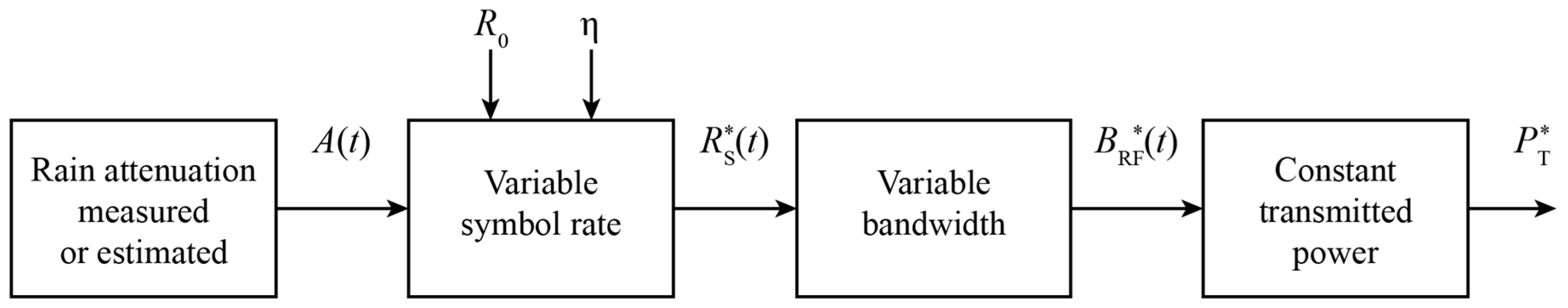
The flow–chart shown in Figure 1 summarizes the theoretical processing necessary to apply the method. Notice, however, that its actual implementation depends on the technology available at the time.

Figure 1.
Flow–chart of the theoretical signal processing necessary for applying the method. The mathematical expressions of the symbols are given in Equations (8) and (9). The actual implementation of the processing depends on the technology of the time.
In the next few sections, we apply these concepts to rain attenuation at 80 GHz, circular polarization, simulated with the SST in zenith paths at the sites listed in Table 1.
3. Link Efficiency in Zenith Paths
We first show the findings on the mean efficiency and, secondly, its application to examples of rain attenuation time series at the sites of Table 1.
3.1. Probability Distributions , and Channel Efficiency
Figure 2 shows the average annual probability distribution of exceeding (mm/h, averaged in 1 min) at the indicated sites. The different climatic conditions of these sites can be clearly observed by comparing the rain rate exceeded with the same probability.
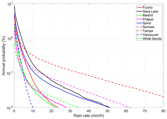
Figure 2.
Annual probability distribution (%) of exceeding the value indicated in abscissa at the indicated sites. Spino d’Adda: continuous blue line; Gera Lario: continuous black line; Fucino: continuous red line; Madrid: continuous green line; Prague: continuous magenta line; Tampa: dashed red line; Norman: dashed magenta line; White Sands: dashed green line; Vancouver: dashed blue line.
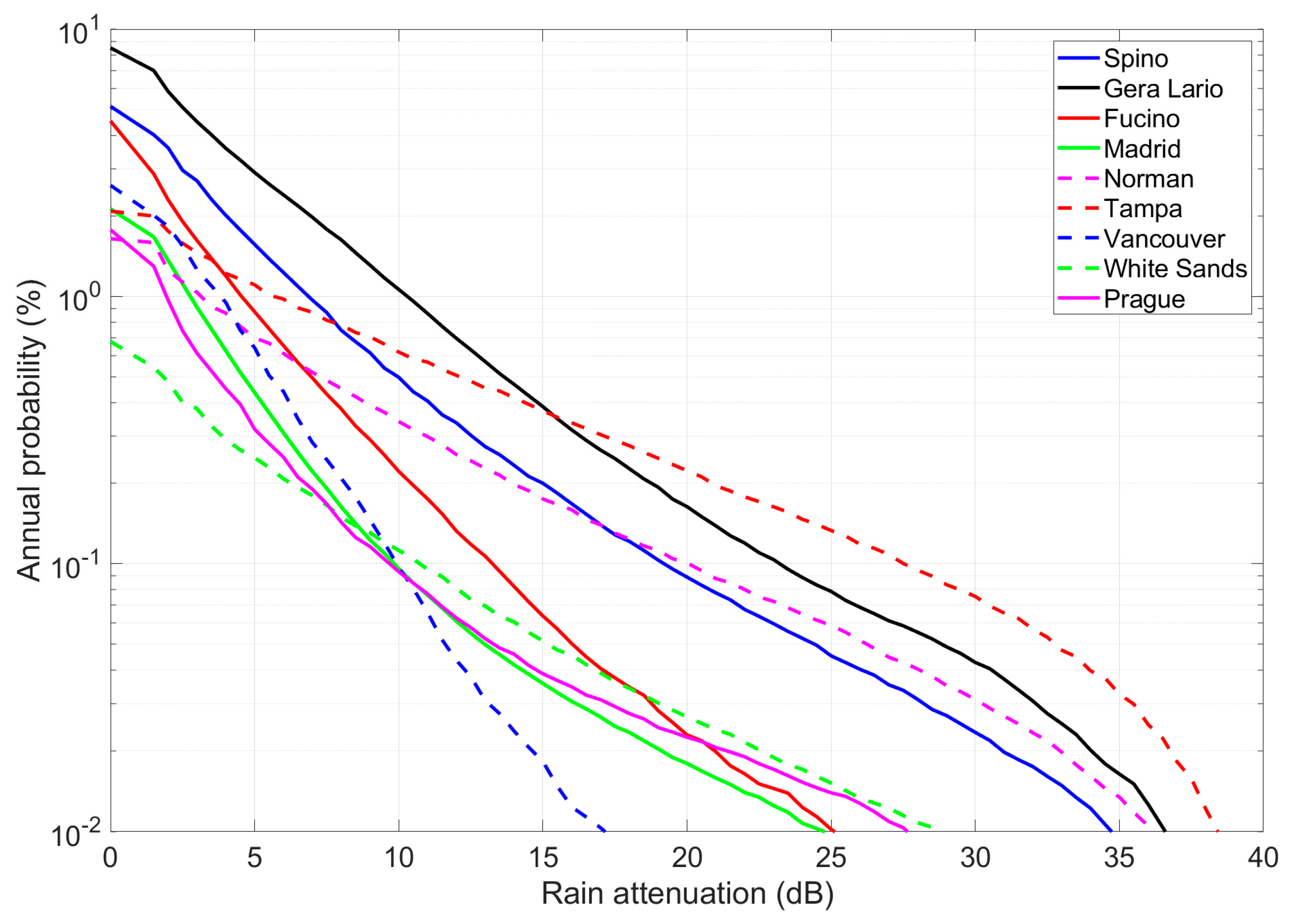
Figure 3 shows the average annual probability distribution of exceeding (dB) in the zenith paths at the indicated sites, simulated with SST (see Equation (29) of [17]). These probability distributions are the data necessary to calculate the mean efficiency and its bounds (Equations (6) and (7)), the power margin (Equation (11)) and the bandwidth expansion factor (Equation (12)).
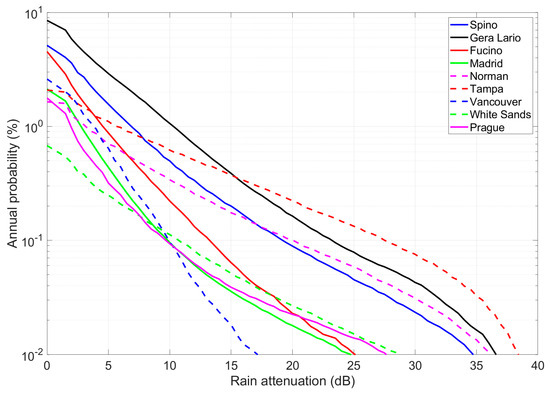
Figure 3.
Annual probability distribution (%) of exceeding the value indicated in abscissa—80 GHz, circular polarization, zenith paths–at the indicated sites. Spino d’Adda: continuous blue line; Gera Lario: continuous black line; Fucino: continuous red line; Madrid: continuous green line; Prague: continuous magenta line; Tampa: dashed red line; Norman: dashed magenta line; White Sands: dashed green line; Vancouver: dashed blue line.
Table 2 reports the mean and minimum (worst–case) efficiency. The mean efficiency ranges from at Tampa (the “worst” site) to at Fucino (the “best” site). Consequently, the power margins—reported in Table 3–and the bandwidth expansion factor—Table 4—are, respectively, dB and 3.77 at Tampa and dB and at Fucino.
Table 2.
Minimum (worst case) and mean values of channel efficiency , Equations (6) and (7), in zenith links working at 80 GHz at the indicated sites.
Table 3.
Maximum (worst case) and mean value of channel power margin factor , (dB), Equation (11), in zenith links working at 80 GHz at the indicated sites.
Table 4.
Maximum (worst case, corresponding to minimum efficiency of Table 2) and mean value of bandwidth expansion factor , Equation (12), in zenith links working at 80 GHz at the indicated sites.
The power margins are always small, well within the capabilities of current technology. The bandwidth expansion factors might be large if the bandwidth in clear—sky conditions is already large; therefore, this might be the most critical issue to consider in relation to practical applications of the method. The evolution of spread-–pectrum technology could ease its application [24,25,26,27,28].
3.2. Examples of Theoretical Application to Time Series
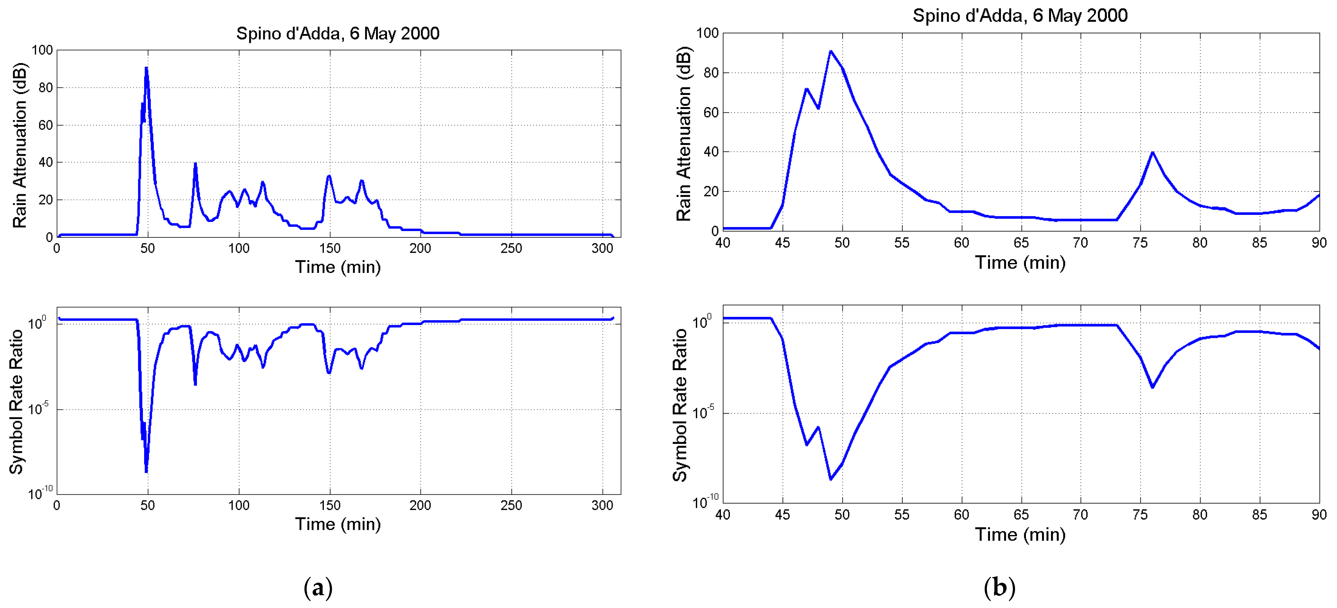
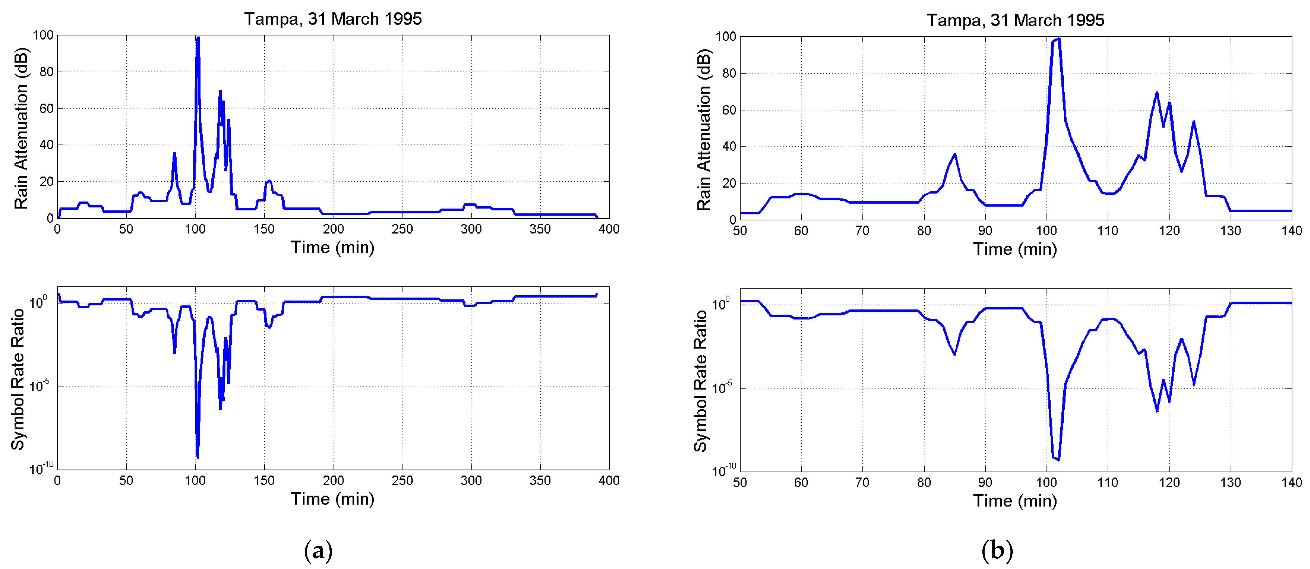
To grasp the time evolution of the symbol rate during a rain attenuation event, Figure 4 and Figure 5 show examples of and , Equation (10), simulated at Spino d’Adda and at Tampa, by adopting the mean efficiency (Table 2). Appendix A reports similar examples for the other sites.
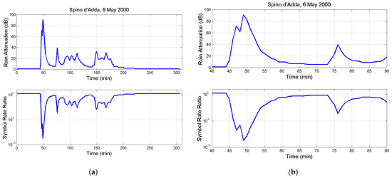
Figure 4.
Upper Panel: (a) Rain attenuation time series : (b) zoom. Lower panel: (a) Symbol rate ratio ; (b) zoom. Spino d’Adda.
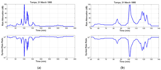
Figure 5.
Upper Panel: (a) Rain attenuation time series : (b) zoom. Lower panel: (a) Symbol rate ratio ; (b) zoom. Tampa.
With straight calculations, we can determine the quantities involved in implementing the method. At Spino d’Adda, at the beginning of the event, i.e., when (Table 4), and at the peak dB (Figure 4). Therefore, for example, if symbols per second, then for long intervals (Figure 4, low attenuation range) the symbol rate would increase to symbols per second. Then, it would decrease smoothly from this value—according to —to reach the minimum value symbols per second at the attenuation peak. This very large range gives a clear indication of the technological issues involved in changing the symbol rate and bandwidth. However, the method promises to avoid the large power margin required for a continuous transmission—up to the fantastic value dB—in conventional design.
Interestingly, in Figure 4 and Figure 5, as well as in Appendix A, regardless of the site, the interval of the onset of a peak is smaller than that of its decay, i.e., the two time–constants are significantly diverse. For example, in Figure 4 (Spino d’Adda), increases from 13.2 dB to the peak 91.0 dB in 5 min, while it decreases to 14.5 dB in 9 min, i.e., with a rate of change dB per minute and dB per minute, respectively. Similar observations can be made for the evolution of the ratio . For Tampa, increases from 13.3 dB to the peak 98.9 dB in 5 min, while it decreases to 14.3 dB in 9 min, i.e., with a rate of change of dB per minute and dB per minute, respectively.
In other words, the intense rainfall causing attenuation peaks fades away more slowly at its end than at its onset; therefore, the long time–scale (several minutes) positive rates of change of attenuation are larger than the negative ones. This behavior at the zenith paths is significantly different than that occurring at slant paths for which the magnitude of positive and negative rates of change is statistically identical, according to the experimental results [29,30,31,32,33] and modeling [34].
In the next section, we consider an evolution of the method by assuming that it is applied in links in which a power margin is already implemented. We show that this fixed power margin is very small.
4. Design with Extra Fixed Power Margin
In Section 3 the method is implemented at the onset of rainfall. In this section, we suppose that a power margin (dB) is already implemented in the link so that the method is applied only in the intervals in which the attenuation threshold is exceeded, i.e., when . The theory recalled in Section 2 can be fully applied to this case by considering the variable and applying Equations (8)–(12) to the conditional probability distribution in which , all calculated from the data drawn in Figure 2. Of course, if , we obtain the results of Section 3.
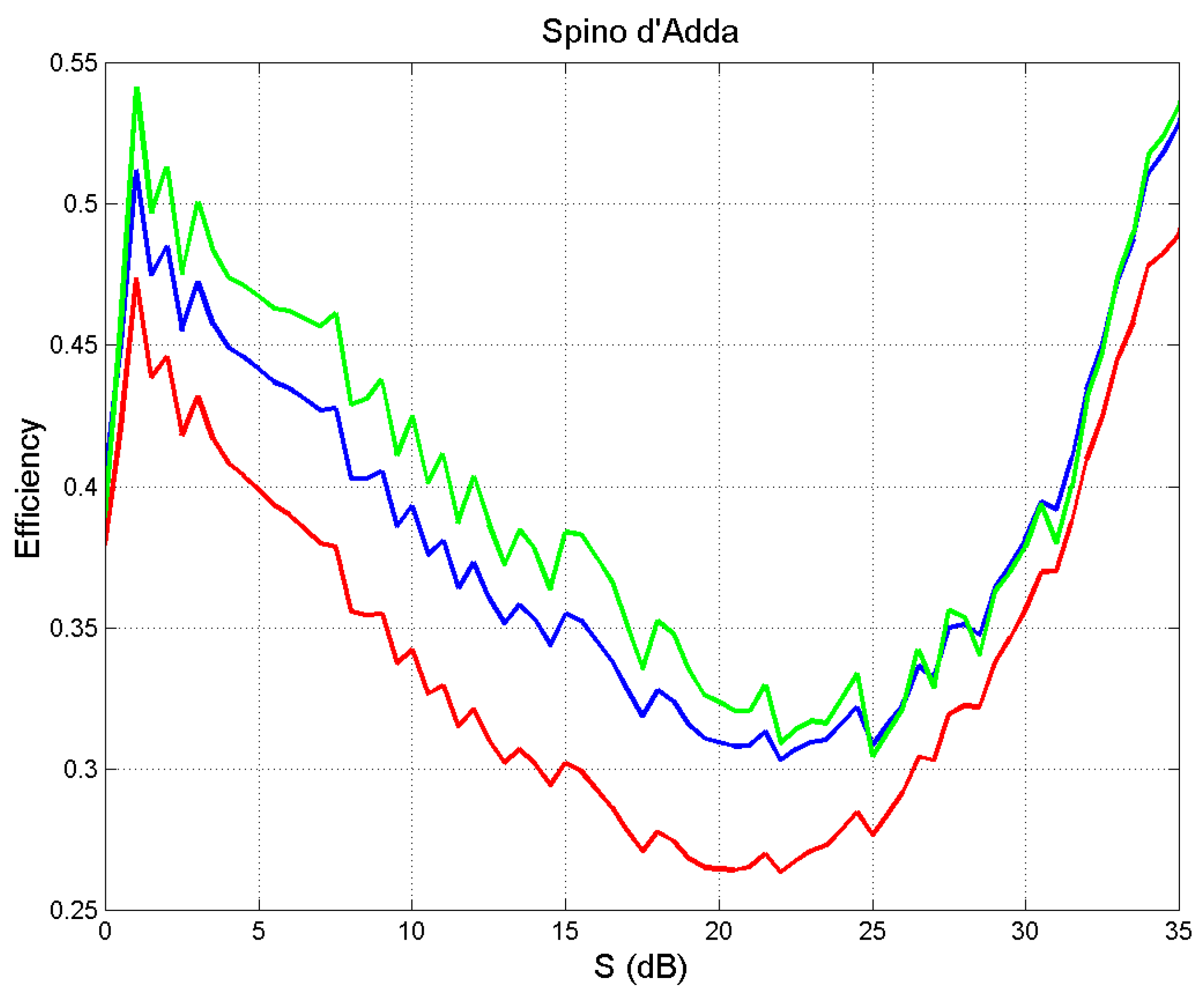
Figure 6 shows the mean and bounds of the efficiency versus , at Spino d’Adda. Figure 7 shows the corresponding values of the extra power margin and Figure 8 shows the corresponding values of the bandwidth expansion factor. Similar curves are obtained for the other sites (these are not shown, for the sake of brevity).
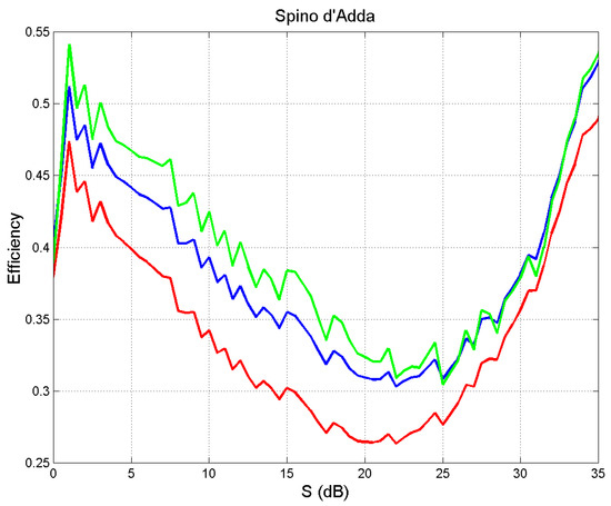
Figure 6.
Mean (blue line) and upper (green line), lower (red line) bounds of the efficiency versus the threshold , at Spino d’Adda.
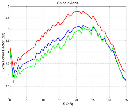
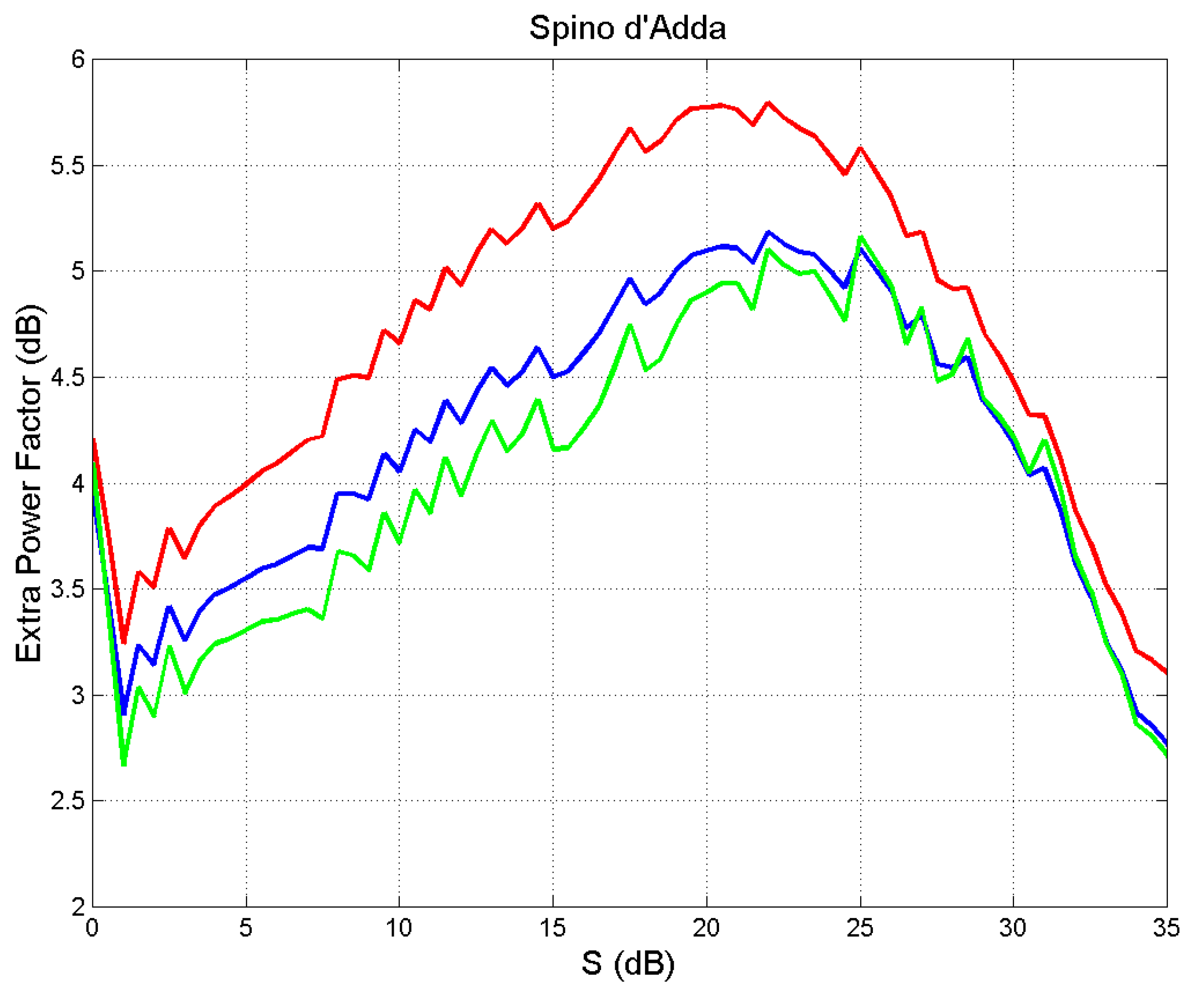
Figure 7.
Extra power factor given by the mean (blue line), upper (green line) and lower (red line) bounds of the efficiency, versus the threshold , at Spino d’Adda.
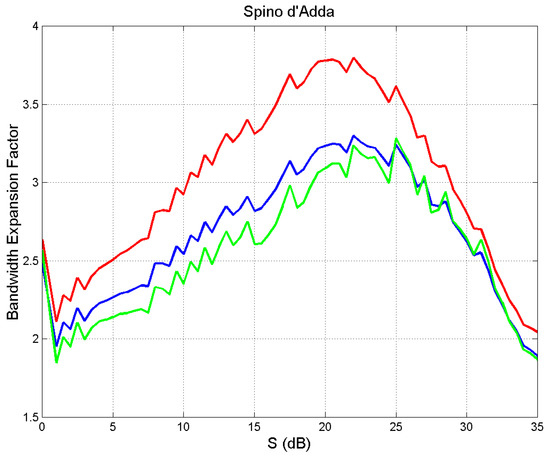
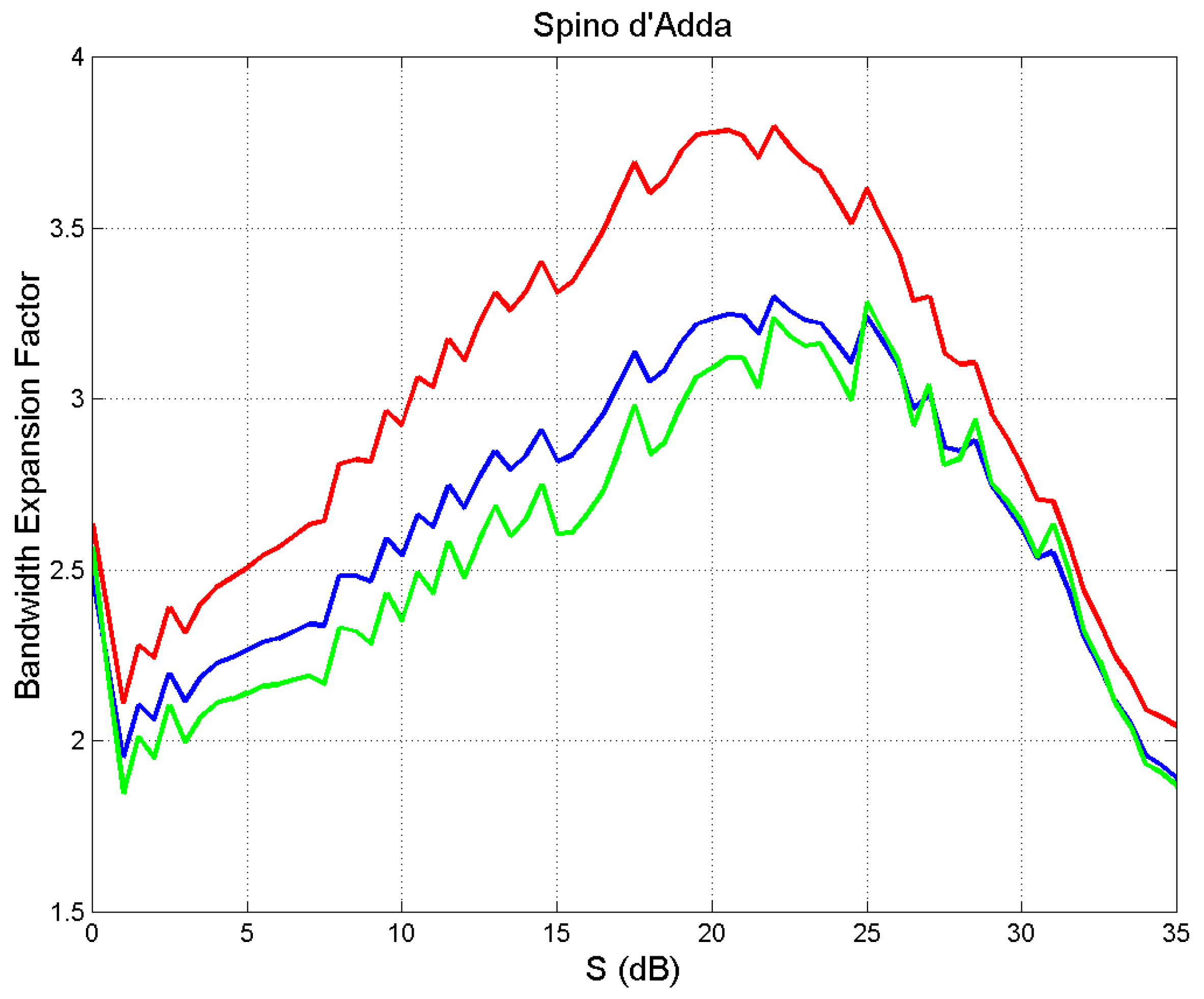
Figure 8.
Maximum bandwidth expansion factor given by the mean (blue line), upper (green line) and lower (red line) bounds of the efficiency, versus the threshold , at Spino d’Adda.
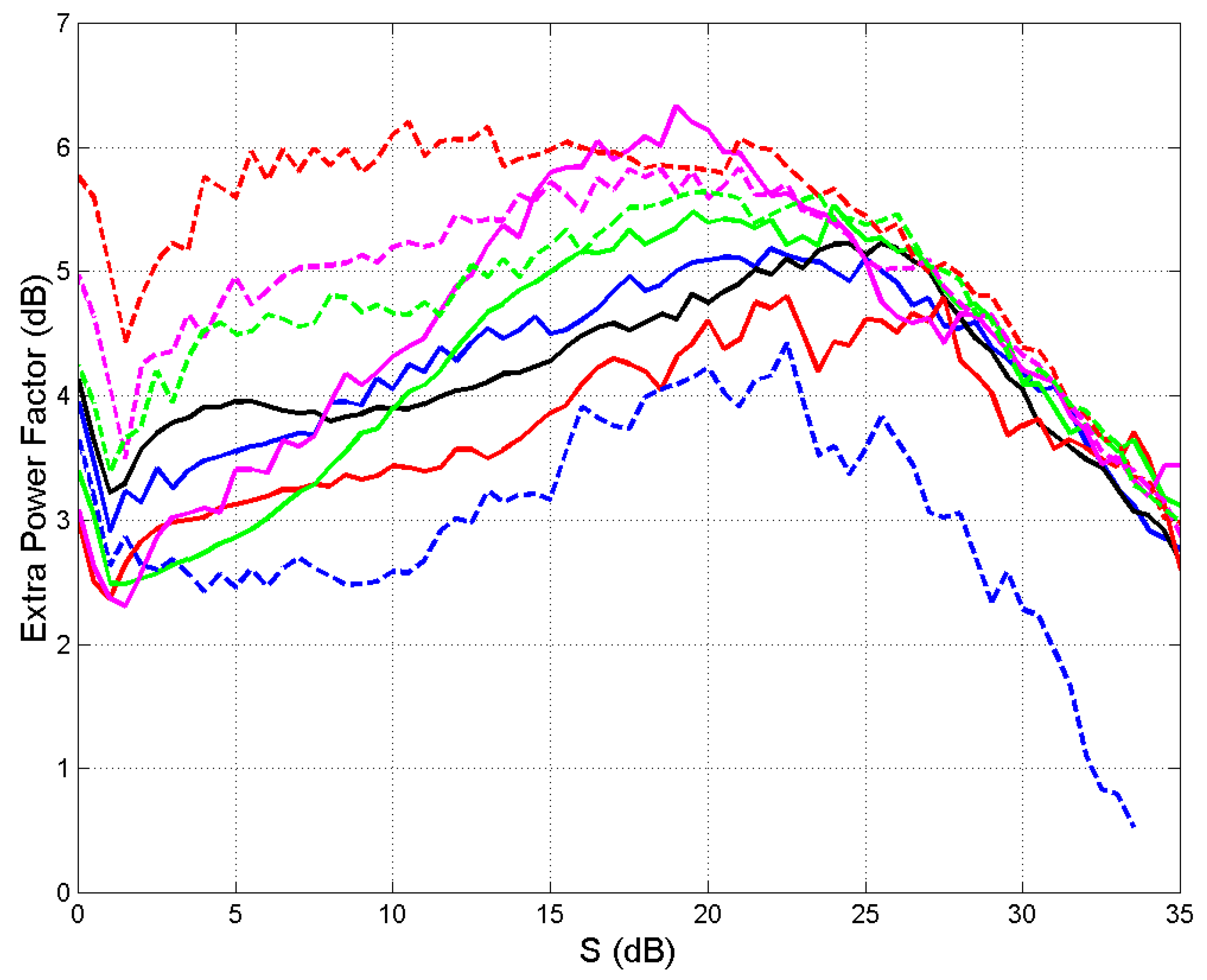
Figure 9 and Figure 10 show the curves obtained for all sites by considering only the mean efficiency. We can observe trends very similar to those of Spino d’Adda, therefore confirming a general behavior of efficiency, and its related parameters, versus . However, differences from site to site are clearly evident, with Tampa being the “worst” site.
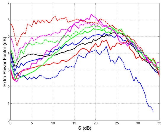
Figure 9.
Extra power factor given by the mean (blue line), upper (green line) and lower (red line) bounds of the efficiency, versus the threshold , at the indicated sites. Spino d’Adda: continuous blue line; Gera Lario: continuous black line; Fucino: continuous red line; Madrid: continuous green line; Prague: continuous magenta line; Tampa: dashed red line; Norman: dashed magenta line; White Sands: dashed green line; Vancouver: dashed blue line.
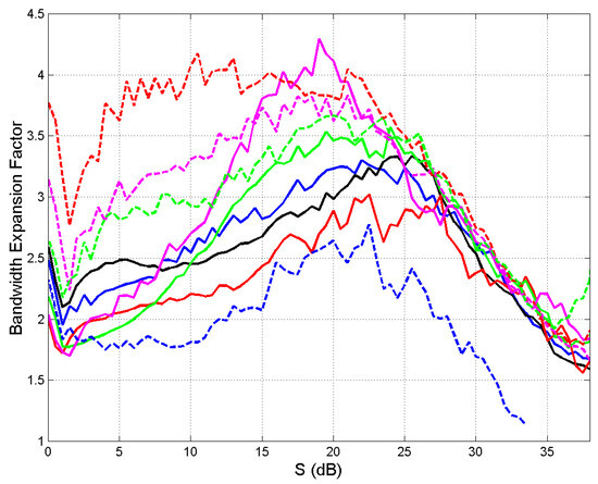
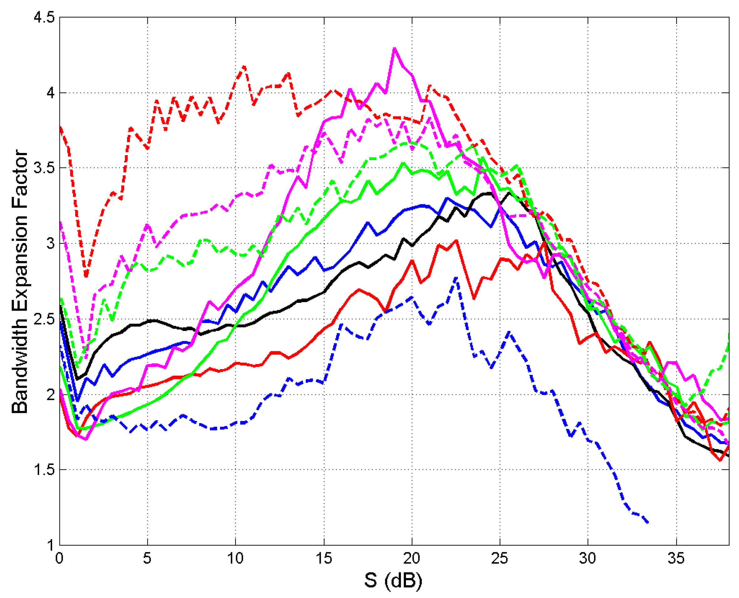
Figure 10.
Maximum bandwidth expansion factor given by the mean (blue line), upper (green line) and lower (red line) bounds of the efficiency, versus the threshold , at the indicated sites. Spino d’Adda: continuous blue line; Gera Lario: continuous black line; Fucino: continuous red line; Madrid: continuous green line; Prague: continuous magenta line; Tampa: dashed red line; Norman: dashed magenta line; White Sands: dashed green line; Vancouver: dashed blue line.
From the figures concerning Spino d’Adda, we can observe the following interesting findings, which are also applicable to all of the other sites:
- (a)
- The efficiency is at its maximum at lower thresholds, but not at dB.
- (b)
- The extra power margin is at its minimum in accordance with efficiency.
- (c)
- The bandwidth expansion factor is at its minimum in accordance with efficiency.
- (d)
- The efficiency is at its minimum (worst case) at about dB.
- (e)
- For dB, another maximum efficiency occurs, but this range is not attractive because of the very large power margin.
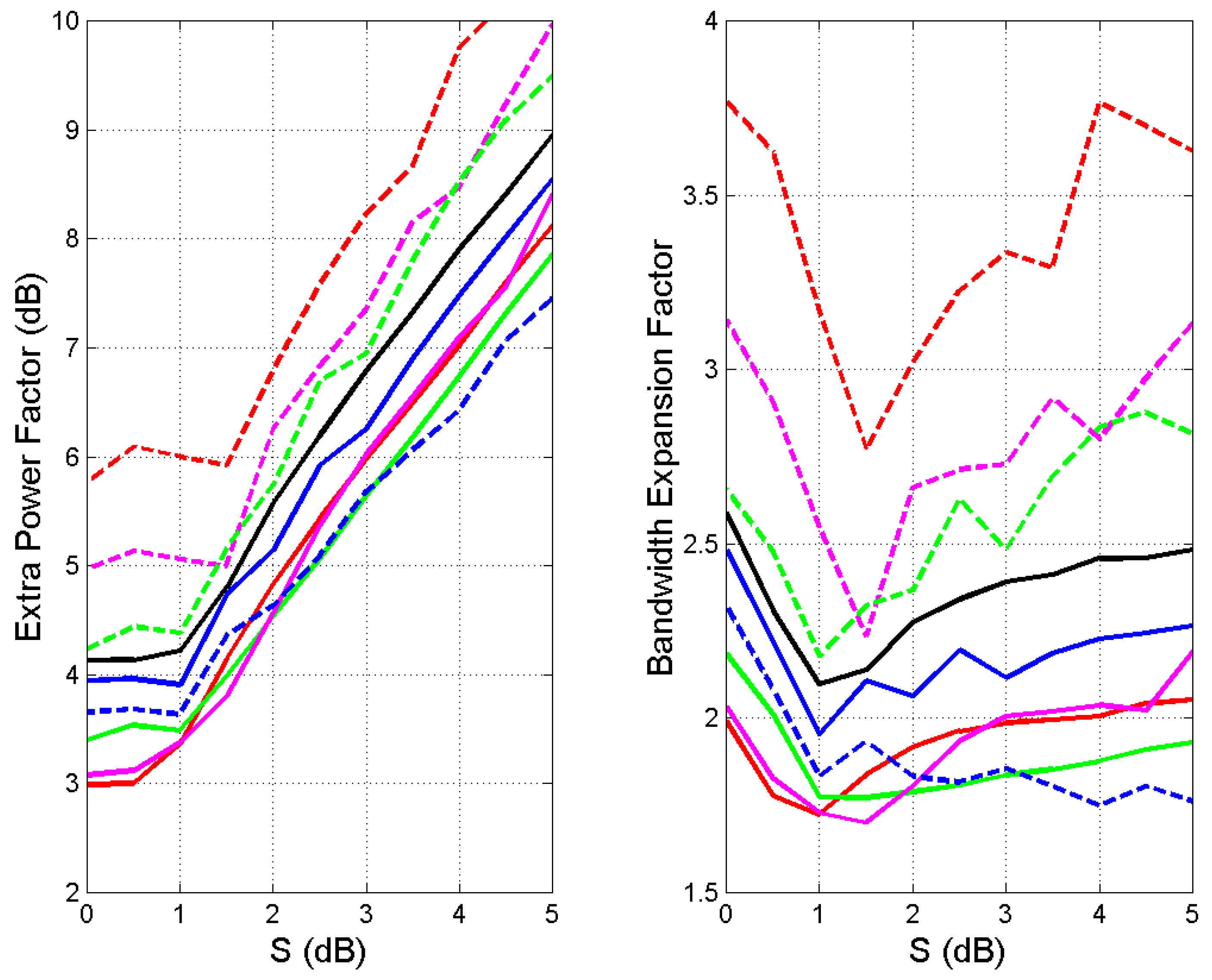
Figure 11 shows details at the low threshold range, which suggests an optimum use of the method. Here, it is interesting to notice that there is no sensible difference in the extra power factor (left panel) in the range dB (right panel), while minima are clearly evident in the bandwidth expansion factor in the range dB. In other words, at any site, the method can be applied when dB, and therefore a power margin dB should be provided before applying the method. For example, for Tampa geographical area (worst site) the final total power margin necessary would be dB, with a bandwidth expansion factor , with dB being the threshold of minimum bandwidth expansion factor (Figure 11, right panel) and dB the extra power factor (Figure 11, left panel).
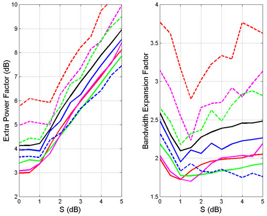
Figure 11.
Left panel: Extra power factor versus the threshold ; Right panel: Maximum bandwidth factor versus the threshold at the indicated sites, details of Figure 8 and Figure 9. Spino d’Adda: continuous blue line; Gera Lario: continuous black line; Fucino: continuous red line; Madrid: continuous green line; Prague: continuous magenta line; Tampa: dashed red line; Norman: dashed magenta line; White Sands: dashed green line; Vancouver: dashed blue line.
Table 5 reports these optimum values for all sites. The total power margin ranges from dB (Norman) to dB (Tampa) and the bandwidth expansion factor ranges from (Prague) to (Tampa). As already observed, the power margin required is very small for all sites, making it well within the capabilities of current technology. The bandwidth expansion factor per se is not very large, but it can be relatively large if the clear—sky bandwidth is already large for the current technology.
Table 5.
Minimum total power margin (dB) and minimum bandwidth expansion factor at the indicated sites, from Figure 11. For example, in the Tampa geographical area, the final total power margin is dB, with a bandwidth expansion factor , being dB the threshold of minimum bandwidth expansion factor (Figure 11, right panel) and dB the extra power factor (Figure 11, left panel).
5. Conclusions
We have recalled that the traditional approach of considering the average probability distribution of rain attenuation is too pessimistic, in terms of power margin, when designing data transfer channels. In fact, if the data volume downloadable during rainfall is more valuable than the instantaneous symbol rate—such as in remote sensing and the internet of things (IoT) using satellites—the method discussed in [6], and summarized in Section 2 of the present paper, can avoid overdesign. However, this method is useful only if (a) data must also be downloaded when it is raining; (b) real—time communication is not strictly required.
The method is characterized only by a single parameter, namely the mean efficiency of the link, and it can transfer the same data volume as if the link were in clear—sky conditions.
In theory, a small power margin and a relatively small bandwidth expansion—regardless of instantaneous rain attenuation—allow us to deliver a mean symbol rate equal to the symbol rate obtainable with no rainfall.
We have applied the method to the links of GeoSurf satellite constellations [16], which have vertical (zenith) paths at any latitude. Since no measurements or predictions are available for zenith paths, we have considered as experimental results the rain attenuation time series simulated at 80 GHz (mm—wave), circular polarization, with the Synthetic Storm Technique [17] from rain—rate time series , recorded on—site for several years.
We have found that the power margins are always small, well within the capabilities of current technology. The maximum bandwidth necessary might be large if the bandwidth in clear—sky conditions is already large; therefore, this might be the most critical issue in practical applications. The evolution of spread—spectrum technology could ease its application.
We have generalized the method by supposing that a small power margin (dB) is already available so that the method is applied only in the intervals in which the attenuation threshold is exceeded, i.e., when . In this case, the total power margin ranges from dB to dB and the bandwidth expansion factor ranges from to . The power margin required is very small for all sites, well within the capabilities of current technology; the bandwidth expansion factor per se is not very large, but it can pose a problem if the clear—sky bandwidth is already large. Future work should assess the sensitivity of the method to errors in matching the theoretical parameters to those measured or simulated with the Synthetic Storm Technique.
Funding
This research received no external funding.
Data Availability Statement
Data are available from the author.
Acknowledgments
Carlo Riva, my colleague at Politecnico di Milano, is gratefully acknowledged for running the SST.
Conflicts of Interest
The author declares no conflicts of interest.
Appendix A
The appendix reports examples of and , at different sites.
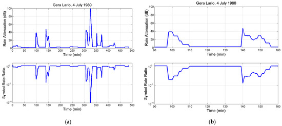
Figure A1.
Upper Panel: (a) Rain attenuation time series : (b) zoom. Lower panel: (a) Symbol rate ratio ; (b) zoom. Gera Lario.
Figure A1.
Upper Panel: (a) Rain attenuation time series : (b) zoom. Lower panel: (a) Symbol rate ratio ; (b) zoom. Gera Lario.
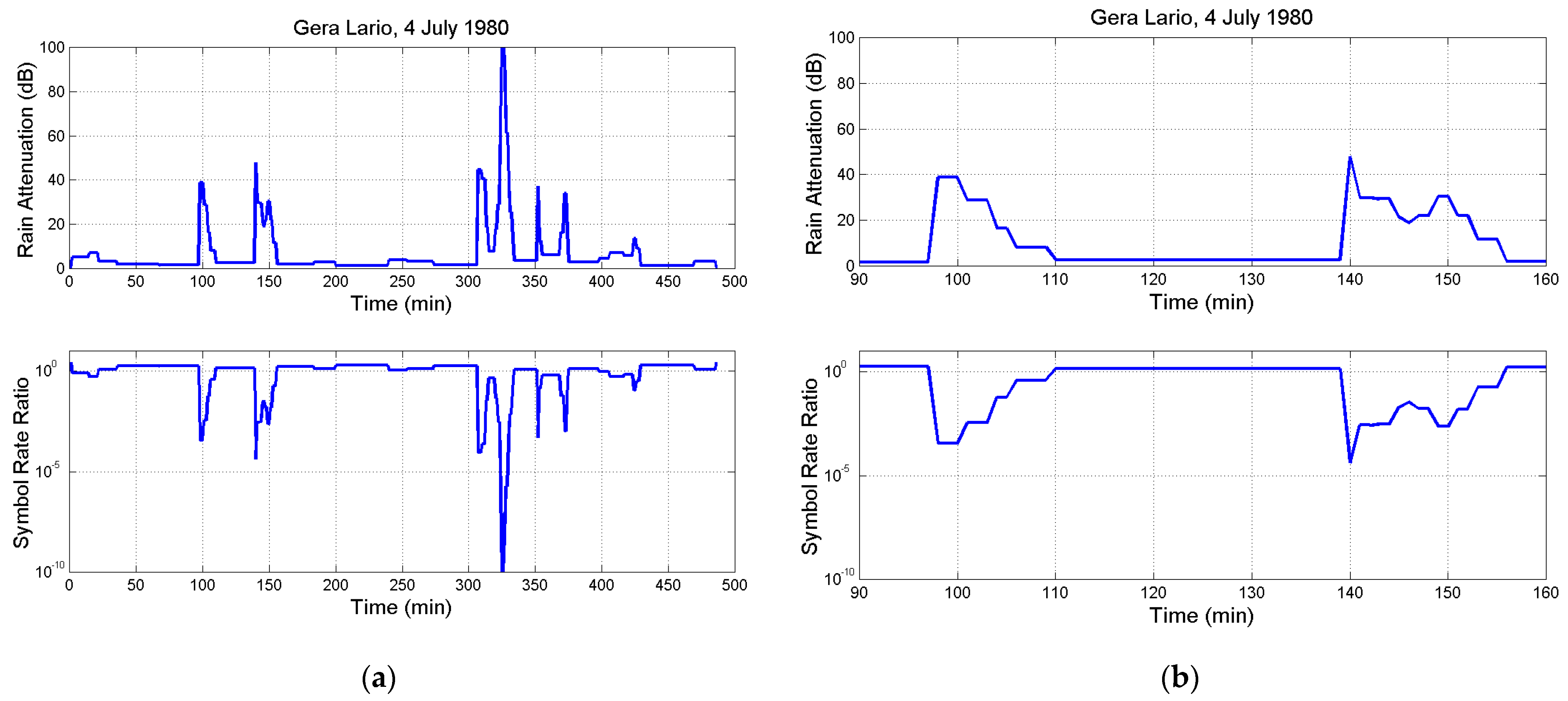
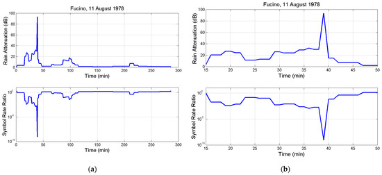
Figure A2.
Upper Panel: (a) Rain attenuation time series : (b) zoom. Lower panel: (a) Symbol rate ratio ; (b) zoom. Fucino.
Figure A2.
Upper Panel: (a) Rain attenuation time series : (b) zoom. Lower panel: (a) Symbol rate ratio ; (b) zoom. Fucino.
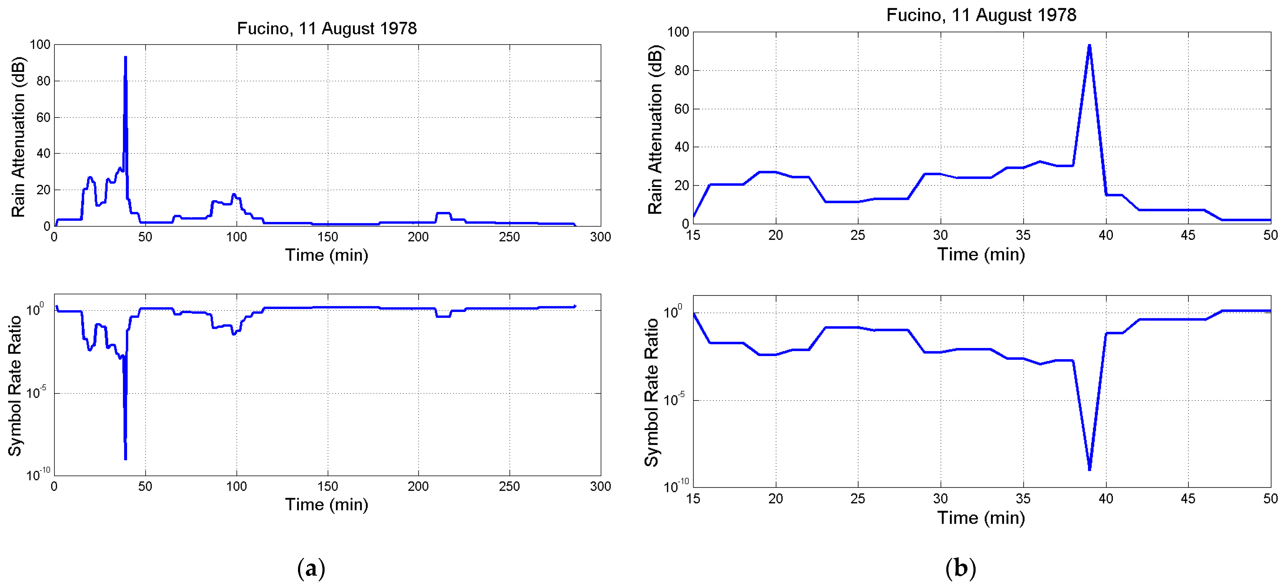
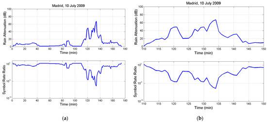
Figure A3.
Upper Panel: (a) Rain attenuation time series : (b) zoom. Lower panel: (a) Symbol rate ratio ; (b) zoom. Madrid.
Figure A3.
Upper Panel: (a) Rain attenuation time series : (b) zoom. Lower panel: (a) Symbol rate ratio ; (b) zoom. Madrid.
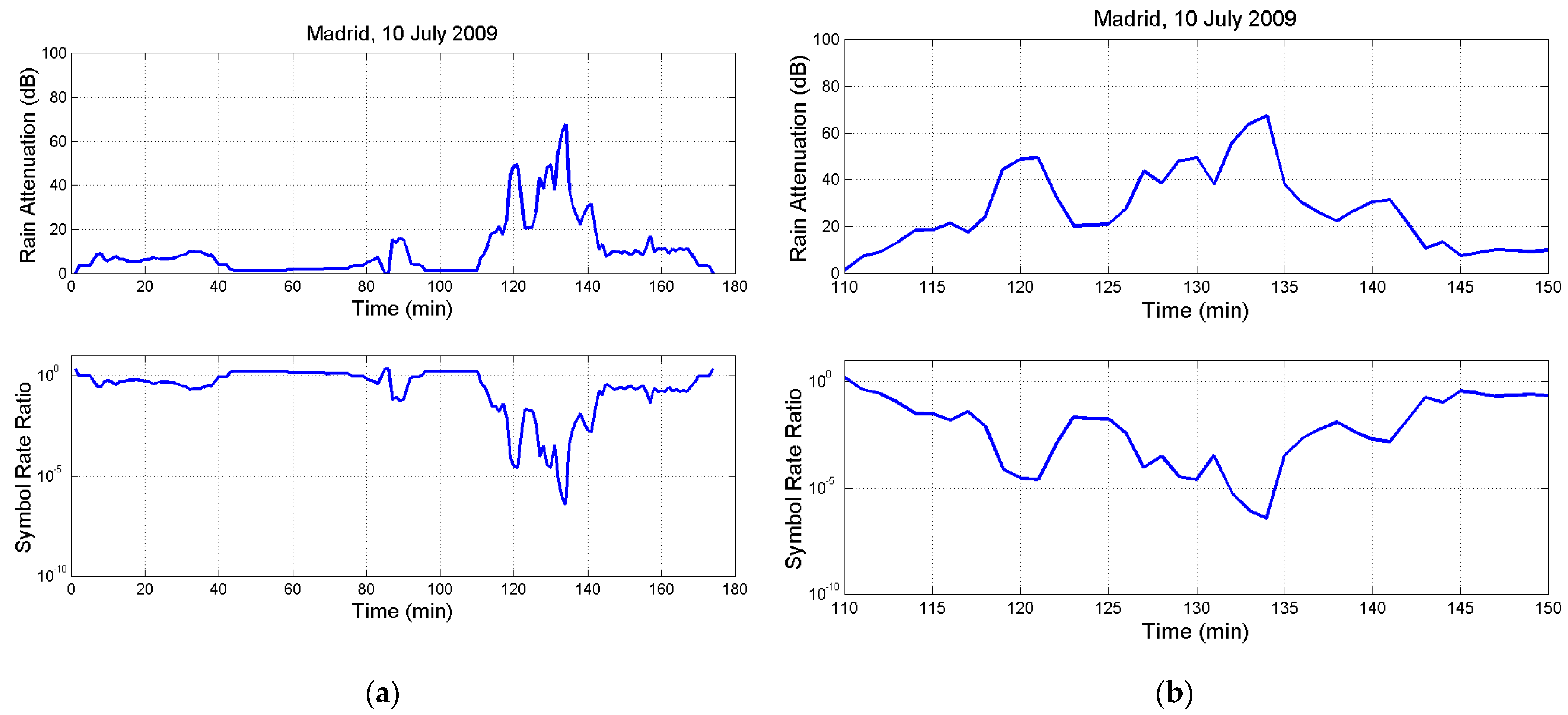
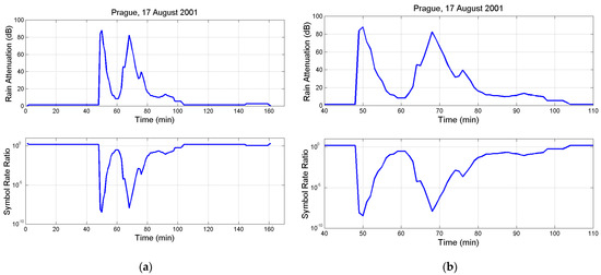
Figure A4.
Upper Panel: (a) Rain attenuation time series : (b) zoom. Lower panel: (a) Symbol rate ratio ; (b) zoom. Prague.
Figure A4.
Upper Panel: (a) Rain attenuation time series : (b) zoom. Lower panel: (a) Symbol rate ratio ; (b) zoom. Prague.
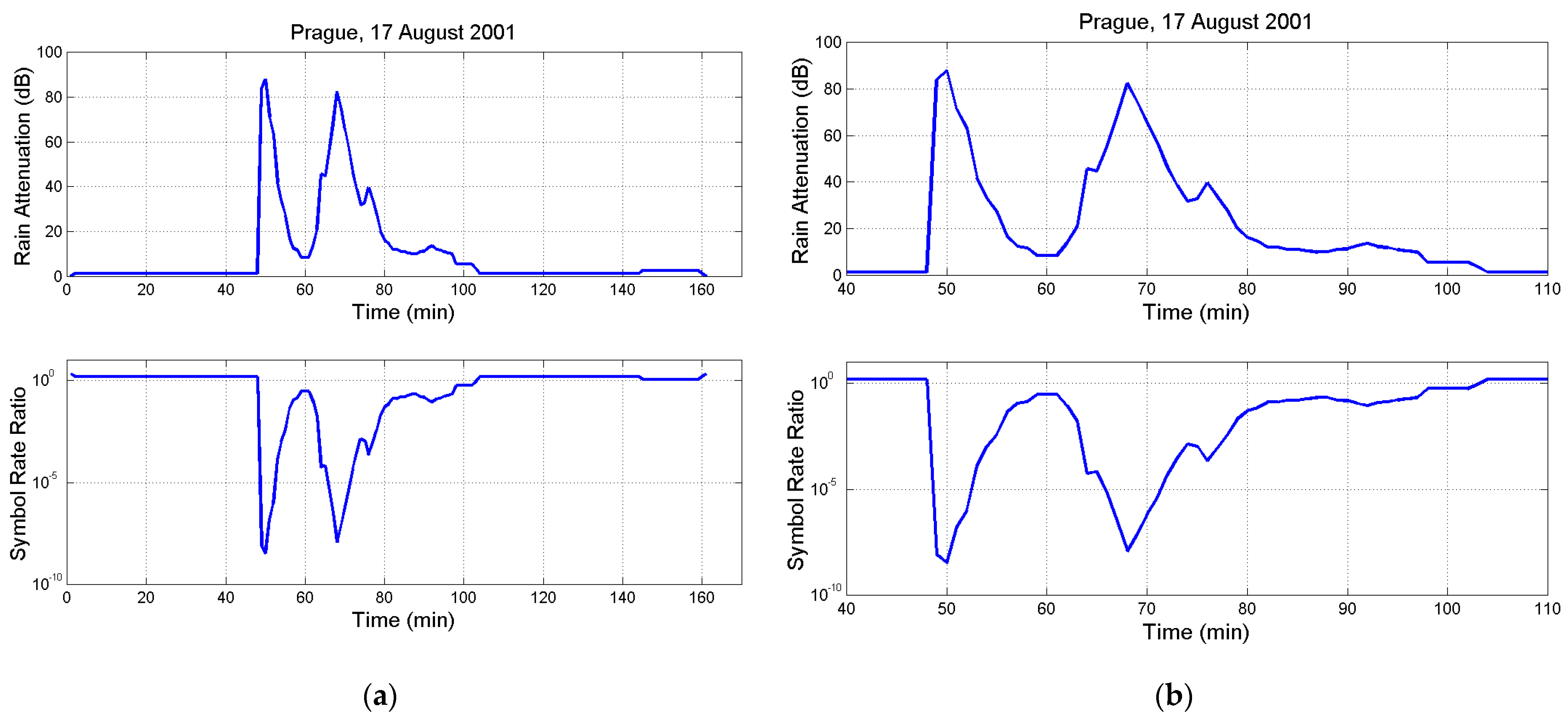
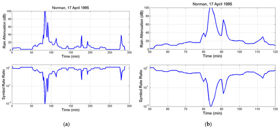
Figure A5.
Upper Panel: (a) Rain attenuation time series : (b) zoom. Lower panel: (a) Symbol rate ratio ; (b) zoom. Norman.
Figure A5.
Upper Panel: (a) Rain attenuation time series : (b) zoom. Lower panel: (a) Symbol rate ratio ; (b) zoom. Norman.
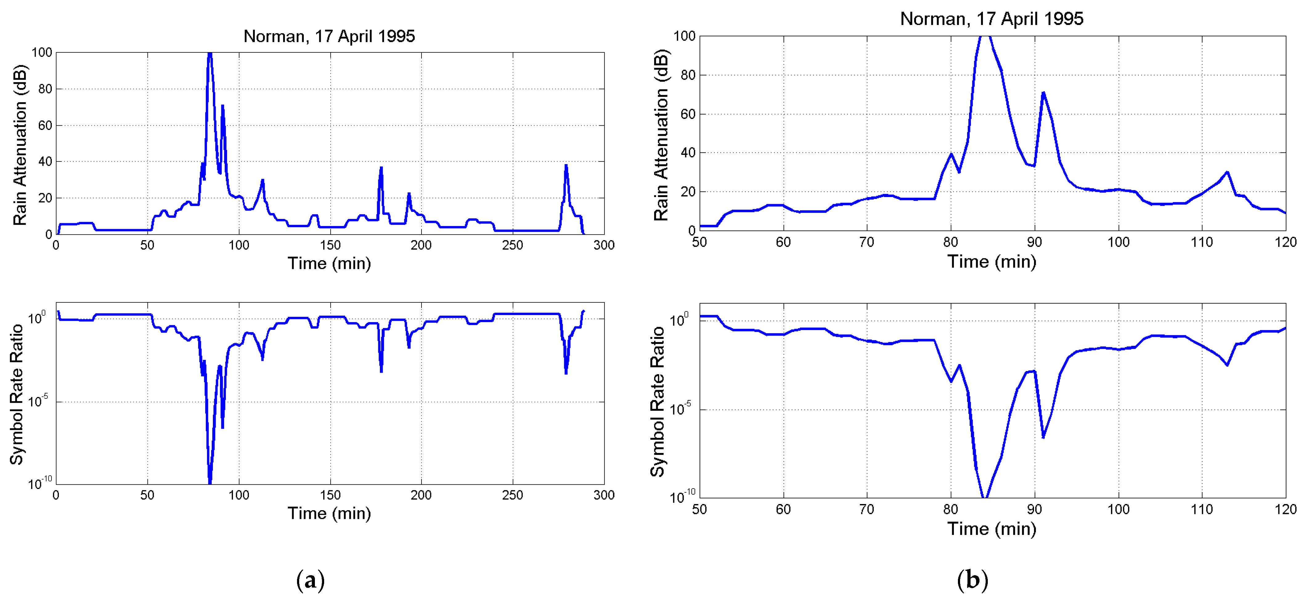
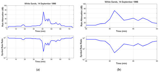
Figure A6.
Upper Panel: (a) Rain attenuation time series : (b) zoom. Lower panel: (a) Symbol rate ratio ; (b) zoom. White Sands.
Figure A6.
Upper Panel: (a) Rain attenuation time series : (b) zoom. Lower panel: (a) Symbol rate ratio ; (b) zoom. White Sands.
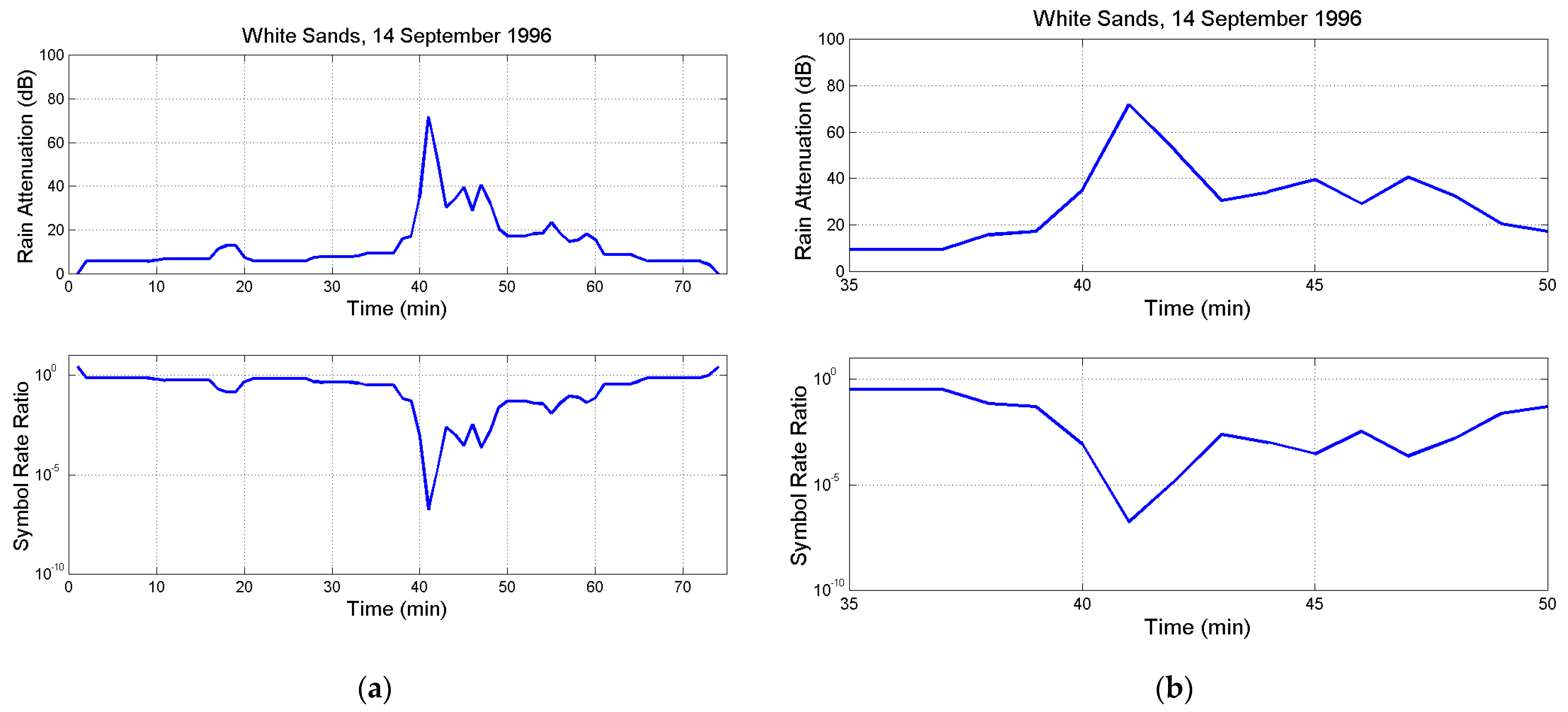
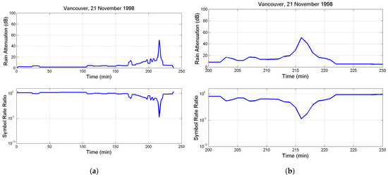
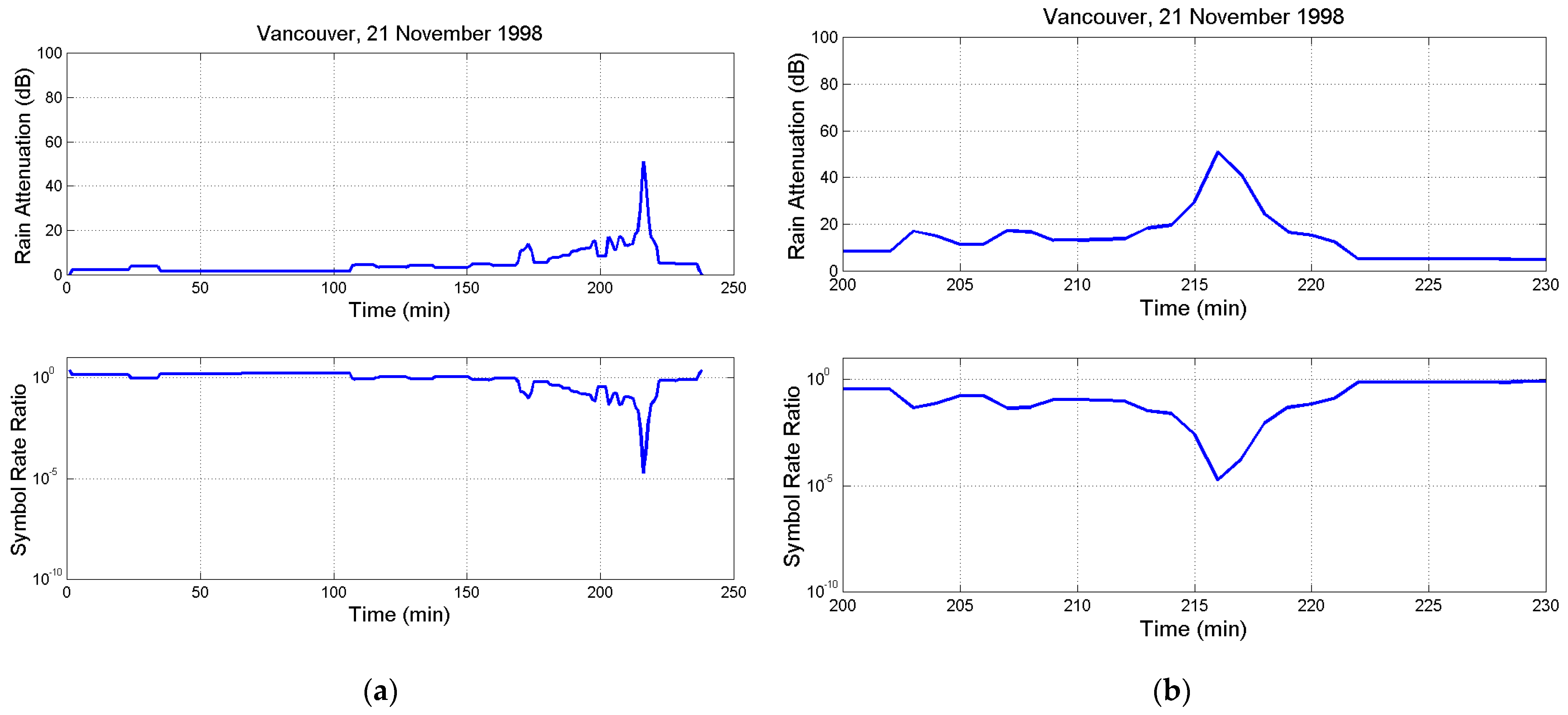
Figure A7.
Upper Panel: (a) Rain attenuation time series : (b) zoom. Lower panel: (a) Symbol rate ratio ; (b) zoom. Vancouver.
Figure A7.
Upper Panel: (a) Rain attenuation time series : (b) zoom. Lower panel: (a) Symbol rate ratio ; (b) zoom. Vancouver.
References
- Matricciani, E.; Riva, C. The search for the most reliable long–Term rain attenuation CDF of a slant path and the impact on prediction models. IEEE Trans. Antennas Propag. 2005, 53, 3075–3079. [Google Scholar] [CrossRef]
- Badron, K.; Ismail, A.F.; Din, J.; Tharek, A.R. Rain induced attenuation studies for V–band satellite communication in tropical region. J. Atmos. Sol. Terr. Phys. 2011, 73, 601–610. [Google Scholar] [CrossRef]
- Boulanger, X.; Gabard, B.; Casadebaig, L.; Castanet, L. Four Years of Total Attenuation Statistics of Earth—Space Propagation Experiments at Ka–Band in Toulouse. IEEE Trans. Antennas Propag. 2015, 63, 2203–2214. [Google Scholar] [CrossRef]
- Kelmendi, A.; Hrovat, A.; Mohorčič, M.; Švigelj, A. Alphasat Propagation Measurements at Ka– and Q–Bands in Ljubljana: Three Years’ Statistical Analysis. IEEE Antennas Wirel. Propag. Lett. 2021, 20, 174–178. [Google Scholar] [CrossRef]
- Propagation Data and Prediction Methods Required for the Design of Earth–Space Telecommunication Systems; Recommendation ITU–R P.618–14; ITU: Geneva, Switzerland, 2023; Volume 8.
- Matricciani, E. A method to achieve clear–Sky data–Volume download in satellite links affected by tropospheric attenuation. Int. J. Satell. Commun. Netw. 2016, 34, 713–723. [Google Scholar] [CrossRef]
- Goldsmith, A.J.; Chua, S.-G. Adaptive Coded Modulation for Fading Channels. IEEE Trans. Commun. 1998, 46, 595–602. [Google Scholar] [CrossRef]
- Andrea, J.; Defever, S.; Moreau, C.; De Gaudenzi, R.; Ginesi, A.; Rinaldo, R.; Gallinaro, G.; Vernucci, A. Adaptive Coding and Modulation for the DVB—S2 Standard Interactive Applications: Capacity Assessment and Key System Issues. IEEE Wirel. Commun. 2007, 14, 61–69. [Google Scholar]
- Bischl, H.; Brandt, H.; de Cola, T.; De Gaudenzi, R.; Eberlein, E.; Girault, N.; Alberty, E.; Lipp, S.; Rinaldo, R.; Rislow, B.; et al. Adaptive coding and modulation for satellite broadband networks: From theory to practice. Int. J. Satell. Commun. Netw. 2010, 28, 59–111. [Google Scholar] [CrossRef]
- Zhang, S.; Yu, G.; Yu, S.; Zhang, Y.; Zhang, Y. Weather–Conscious Adaptive Modulation and Coding Scheme for Satellite—Related Ubiquitous Networking and Computing. Electronics 2022, 11, 1297. [Google Scholar] [CrossRef]
- Wang, Z.; Lu, F.; Wang, D.; Zhang, X.; Li, J.; Li, J. A Transmission Efficiency Evaluation Method of Adaptive Coding Modulation for Ka—Band Data—Transmission of LEO EO Satellites. Sensors 2022, 22, 5423. [Google Scholar] [CrossRef] [PubMed]
- Mhangara, P.; Mapurisa, W. Multi–Mission earth observation data processing system. Sensors 2019, 19, 3831. [Google Scholar] [CrossRef]
- Yang, X.Q.; Li, L.; Jin, F.; Zhang, J.P. Research on satellite–Borne high–Speed adaptive transmission technique. Space Electron. Technol. 2014, 11, 20–24. [Google Scholar]
- Zhang, J.P. Adaptive coding and modulation for remote sensing satellite. Space Electron. Technol. 2016, 13, 78–86. [Google Scholar]
- Wang, Z.G.; Wang, D.B.; Hu, Y.; Lu, F. Analysis on application efficiency of adaptive coding and modulation for LEO remote sensing satellite at Ka—Band. Spacecr. Eng. 2021, 30, 69–76. [Google Scholar]
- Matricciani, E. Geocentric Spherical Surfaces Emulating the Geostationary Orbit at Any Latitude with Zenith Links. Future Internet 2020, 12, 16. [Google Scholar] [CrossRef]
- Matricciani, E. Physical-mathematical model of the dynamics of rain attenuation based on rain rate time series and a two-layer vertical structure of precipitation. Radio Sci. 1996, 31, 281–295. [Google Scholar] [CrossRef]
- Matricciani, E. Prediction of fade duration due to rain in satellite communication systems. Radio Sci. 1997, 22, 935–941. [Google Scholar] [CrossRef]
- Chakraborty, S.; Verma, P.; Paudel, B.; Shukla, A.; Das, S. Validation of Synthetic Storm Technique for Rain Attenuation Prediction Over High–Rainfall Tropical Region. IEEE Geosci. Remote Sens. Lett. 2021, 19, 1002104. [Google Scholar] [CrossRef]
- Jong, S.L.; Riva, C.; D’Amico, M.; Lam, H.Y.; Yunus, M.M.; Din, J. Performance of synthetic storm technique in estimating fade dynamics in equatorial Malaysia. Int. J. Satell. Commun. Netw. 2018, 36, 416–426. [Google Scholar] [CrossRef]
- Nandi, D.D.; Pérez-Fontán, F.; Pastoriza-Santos, V.; Machado, F. Application of synthetic storm technique for rain attenuation prediction at Ka and Q band for a temperate Location, Vigo, Spain. Adv. Space Res. 2020, 66, 800–809. [Google Scholar] [CrossRef]
- Matricciani, E.; Riva, C. Duration of Rainfall Fades in GeoSurf Satellite Constellations. Appl. Sci. 2024, 14, 1865. [Google Scholar] [CrossRef]
- Marzano, F.S. Modeling antenna noise temperature due to rain clouds at microwave and millimeter–wave frequencies. IEEE Trans. Antennas Propag. 2006, 54, 1305–1317. [Google Scholar] [CrossRef]
- Turin, G.L. Introduction to spread spectrum antimultipath techniques and their application to urban digital radio. Proc. IEEE 1980, 68, 328–353. [Google Scholar] [CrossRef]
- Pickholtz, R.; Schilling, D.; Milstein, L. Theory of spread-spectrum communications—A tutorial. IEEE Trans. Commun. 1982, 30, 855–884. [Google Scholar] [CrossRef]
- Viterbi, A.J. CDMA Principles of Spread Spectrum Communications; Addinson-Wesly: Reading, MA, USA, 1995. [Google Scholar]
- Dinan, E.H.; Jabbari, B. Spreading codes for direct sequence CDMA and wideband CDMA celluar networks. IEEE Commun. Mag. 1998, 36, 48–54. [Google Scholar] [CrossRef]
- Veeravalli, V.V.; Mantravadi, A. The coding–Spreading trade–Off in CDMA systems. IEEE Trans. Sel. Areas Commun. 2002, 20, 396–408. [Google Scholar] [CrossRef]
- Garcia-Rubia, J.M.; Riera, J.M.; Garcia-Del-Pino, P.; Pimienta-del-Valle, D.; Siles, G.A. Fade and Interfade Duration Characteristics in a Slant–Path Ka–Band Link. IEEE Trans. Antennas Propag. 2017, 65, 7198–7206. [Google Scholar] [CrossRef]
- Chakraborty, S.; Chakraborty, M.; Das, S. Second order experimental statistics of rain attenuation at Ka band in a tropical location. Adv. Space Res. 2012, 67, 4043–4053. [Google Scholar] [CrossRef]
- Papafragkakis, A.Z.; Kourogiorgas, C.I.; Panagopoulos, A.D.; Ventouras, S. Second Order Excess Attenuation Statistics in Athens, Greece at 19.701 GHz using ALPHASAT. In Proceedings of the 12th International Symposium on Communication Systems, Networks and Digital Signal Processing (CSNDSP), Porto, Portugal, 20–22 July 2020. [Google Scholar] [CrossRef]
- Das, S.; Chakraborty, M.; Chakraborty, S.; Shukla, A.; Acharya, R. Experimental studies of Ka Band Rain Fade Slope at a Tropical Location of India. Adv. Space Res. 2020, 66, 1551–1557. [Google Scholar] [CrossRef]
- Jong, S.L.; Riva, C.; Din, J.; D’Amico, M.; Lam, H.Y. Fade slope analysis for Ku-band earth-space communication links in Malaysia. IET Microw. Antennas Propag. 2019, 13, 2330–2335. [Google Scholar] [CrossRef]
- Samad, M.A.; Diba, F.D.; Choi, D.-Y. A Survey of Rain Fade Models for Earth–Space Telecommunication Links–Taxonomy, Methods, and Comparative Study. Remote Sens. 2021, 13, 1965. [Google Scholar] [CrossRef]

Disclaimer/Publisher’s Note: The statements, opinions and data contained in all publications are solely those of the individual author(s) and contributor(s) and not of MDPI and/or the editor(s). MDPI and/or the editor(s) disclaim responsibility for any injury to people or property resulting from any ideas, methods, instructions or products referred to in the content. |
© 2024 by the author. Licensee MDPI, Basel, Switzerland. This article is an open access article distributed under the terms and conditions of the Creative Commons Attribution (CC BY) license (https://creativecommons.org/licenses/by/4.0/).