Advanced Anomaly Detection in Manufacturing Processes: Leveraging Feature Value Analysis for Normalizing Anomalous Data

Abstract

In the realm of manufacturing processes, equipment failures can result in substantial financial losses and pose significant safety hazards. Consequently, prior research has primarily been focused on preemptively detecting anomalies before they manifest. However, within industrial contexts, the precise interpretation of predictive outcomes holds paramount importance. This has spurred the development of research in Explainable Artificial Intelligence (XAI) to elucidate the inner workings of predictive models. Previous studies have endeavored to furnish explanations for anomaly detection within these models. Nonetheless, rectifying these anomalies typically necessitates the expertise of seasoned professionals. Therefore, our study extends beyond the mere identification of anomaly causes; we also ascertain the specific adjustments required to normalize these deviations. In this paper, we present novel research avenues and introduce three methods to tackle this challenge. Each method has exhibited a remarkable success rate in normalizing detected errors, scoring 97.30%, 97.30%, and 100.0%, respectively. This research not only contributes to the field of anomaly detection but also amplifies the practical applicability of these models in industrial environments. It furnishes actionable insights for error correction, thereby enhancing their utility and efficacy in real-world scenarios.

1. Introduction

This research highlights the significant challenges facing the manufacturing industry, particularly the costly problems caused by equipment failures in the manufacturing process and the limitations of human experience and knowledge, which are largely relied upon to solve these problems [1,2]. Product defects in new equipment and frequent process stoppages due to equipment anomalies pose a serious threat to worker safety and underscore the need for data-driven quality failure prediction systems to address these issues. While much of the current research is focused on using in-process data to predict failures, there is relatively little research on Explainable Artificial Intelligence (XAI) for clarifying and resolving the causes of failures when they occur. Furthermore, existing XAI that has been studied in manufacturing simply suggests the most relevant features [3,4]. The knowledge of how to modify certain features to normalize the quality of a product still relies heavily on experienced experts [5]. These issues suggest that in order to improve efficiency and safety on the industrial floor, solutions should be sought through data-driven analytics and increased transparency of artificial intelligence. In this study, AI techniques were applied to perform anomaly detection of products based on various variables available in the manufacturing industry, such as temperature, voltage, current, injection time, etc. [6]. When a product is predicted to be defective, relevant features were identified to understand what factors led to the prediction. The method proposed in this study is an ensemble tree-based method for selecting features based on the mode value of nodes, which was compared with the existing SHapley Additive exPlanation (SHAP)-based feature detection method. Furthermore, this study proposes a methodology that goes beyond simply identifying the key features that are anomalous but also proposes a methodology for how much the features should be modified to normalize the product. This study proposes three methods: a SHapley Additive exPlanation (SHAP) method, a method using the most frequent node, and a method using conditional statements at the end node that ultimately influences the decision. This study found that these methods achieved normalization rates of 97.30%, 97.30%, and 100.0%, respectively. This paper is organized as follows: First, in Section 2, we describe the machine learning used in our paper, including prior work on anomaly detection in manufacturing processes, and SHAP, a type of XAI. Then, in Section 3, we describe the data we used and show how we processed the data and how we performed the outlier detection using different machine learning models. Finally, we present our interpretation of what input variables caused the outlier data, which is the most important aspect of our work, and how we propose to modify them to normalize them. Section 4 evaluates how well the proposed normalization methods work in practice, followed by a discussion in Section 5, and this paper concludes with further analysis and conclusions in Section 6.

2. Related Works

2.1. Preliminary Research on Predicting Anomaly Data on the Factory Floor

Several studies have been conducted on proactive manufacturing sites. Paul et al. proposed a series AC arc fault detection method based on Random Forests, achieving simplicity and high accuracy compared to conventional ANN- and DNN-based algorithms [7,8,9]. This method employed grid search algorithms for hyperparameter tuning and precision–recall trade-off analysis to find the optimal classification threshold. However, it relies on traditional machine learning models that may lack transparency in the decision making process. This opacity can make it difficult to interpret why certain features are considered important, especially in complex manufacturing settings where understanding the root cause of defects is crucial for actionable insights. Fang et al. introduced a machine learning approach for anomaly detection in intelligent bearing fault diagnosis of power mixing equipment [10]. This method utilized features such as wavelet packet transformation for vibration-based analysis and extraction, combined with genetic/Particle Swarm optimization for feature selection, showing high efficiency and accuracy in detecting bearing and gear defects. However, these feature extraction and optimization techniques can contribute to the complexity of the model, making it difficult for decision-makers to interpret the model’s predictions and understand the underlying reasons for specific anomalies. Additionally, the computational complexity of the model may limit its applicability in real-time scenarios. Li et al. used a novel machine learning model called deep forest to predict the risk of rockburst [11]. Deep forest, integrating the characteristics of deep learning and ensemble models, demonstrated the ability to address the complex and unpredictable nature of rockbursts, using Bayesian optimization methods to adjust the hyperparameters of the model [12]. While this model exhibited outstanding accuracy, its narrow focus on underground rock engineering limits its applicability. Furthermore, the high accuracy in controlled test scenarios may not fully translate to real-world settings where data can be noisier and conditions more variable.

2.2. Machine Learning Models

For predicting the quality of manufacturing data, various classifiers were employed: K-Nearest Neighbors Classifier [13,14], Decision Trees Classifier [15,16], Random Forest Classifier [17,18], Extra Trees Classifier [19,20], and Gradient Boosting Classifier [21,22]. The K-Nearest Neighbors Classifier operates by classifying or predicting based on the k-nearest neighboring data points to a given data point, offering an intuitive approach but suffering from increased computational costs as the dataset size grows. The Decision Trees Classifier segments data through ’if-then-else’ decision rules, making decisions on features at each node, representing the outcomes of those decisions at each branch, and repeating the process until a pure subset is derived or a specified maximum depth is reached. The core idea of the Random Forest Classifier is to combine multiple decision trees to reduce the overfitting issue of individual trees and enhance the overall model’s generalization ability. Each decision tree is trained on a random subset of the data, and the final outcome is determined by selecting the class most frequently chosen by the trees. The Extra Trees Classifier is a variation of Random Forest that increases randomness to decrease overfitting. It builds trees using randomly selected data subsets and random splits rather than searching for the optimal split, thereby reducing computational costs and speeding up the learning process. The Gradient Boosting Classifier sequentially trains multiple weak predictors and assembles them into a robust prediction model. At each stage, new models are added in a direction that reduces the errors of the previous models, and the model’s performance is continuously enhanced by adjusting the weights in a direction that minimizes the loss function of the model, utilizing gradient descent.

2.3. SHAP

In modeling for improving defect rates in the manufacturing process, identifying causal factors and understanding their impact on the results is crucial. One of the tools enabling such explainability in results is the eXplainable AI method known as SHapley Additive exPlanation (SHAP) [23]. Figure 1 below represents the entire process of SHAP.

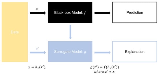
Figure 1. Overview of SHAP methodology.

Initially, there is a black-box model f and its corresponding predictions [24]. Instead of using identical input values, simplified input values are used to find a Surrogate model g that satisfies $g\left(z^{\prime }\right)=f\left(h_x\left(z^{\prime }\right)\right)$ [25]. Essentially, the Surrogate model uses transformed inputs to generate outputs similar to those provided by the original black-box model. SHAP is model-agnostic and distributes the impact of each feature additively, not only for the overall model feature importance but also for the influence of each feature on individual prediction values. In other words, SHAP represents the impact of specific variables on individual predictions as the sum of the influences of the actually existing variables. The Shapley Value is used as the metric for measuring this influence, offering an additive feature importance measure that satisfies three properties of feature attribution: Local Accuracy, Missingness, and Consistency. For tree-based models like Random Forest and Gradient Boosting Machine, Tree SHAP is utilized [26]. Traditional methods of measuring feature importance in Tree Ensemble Models, such as Gain [27] and Split Count [28], have limitations due to their inconsistency across models or individual trees. It is unreliable if feature importance varies even though models are trained from the same data. However, SHAP allows for the computation of consistent feature importance regardless of the order of splits.

3. Method

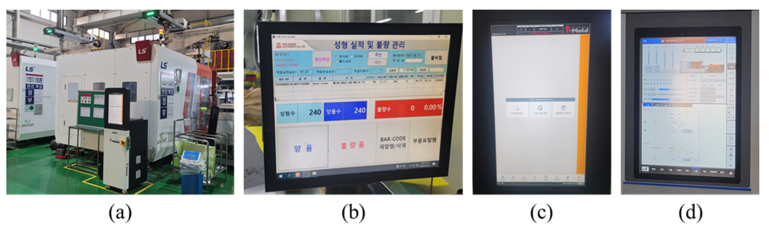
The data utilized in this study were collected from plastic injection manufacturing equipment employing a physical foaming molding method. This equipment incorporates a novel technology, specifically a chemical foaming molding method, and utilizes an eco-friendly manufacturing technique that reduces the use of plastic raw materials (resin) and enables the use of recycled resin. An example of the injection equipment can be observed in Figure 2.

Figure 2. Examples of plastic injection manufacturing equipment: (a) Equipment for injection targeting. (b) Performance and defect management equipment. (c) Injection model application equipment. (d) Data collection and management equipment.

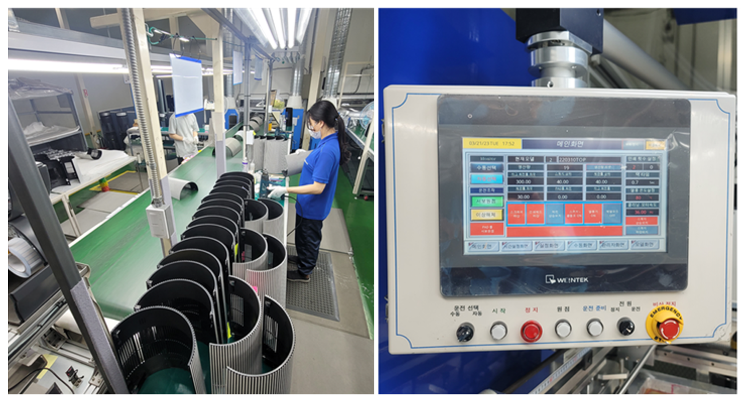
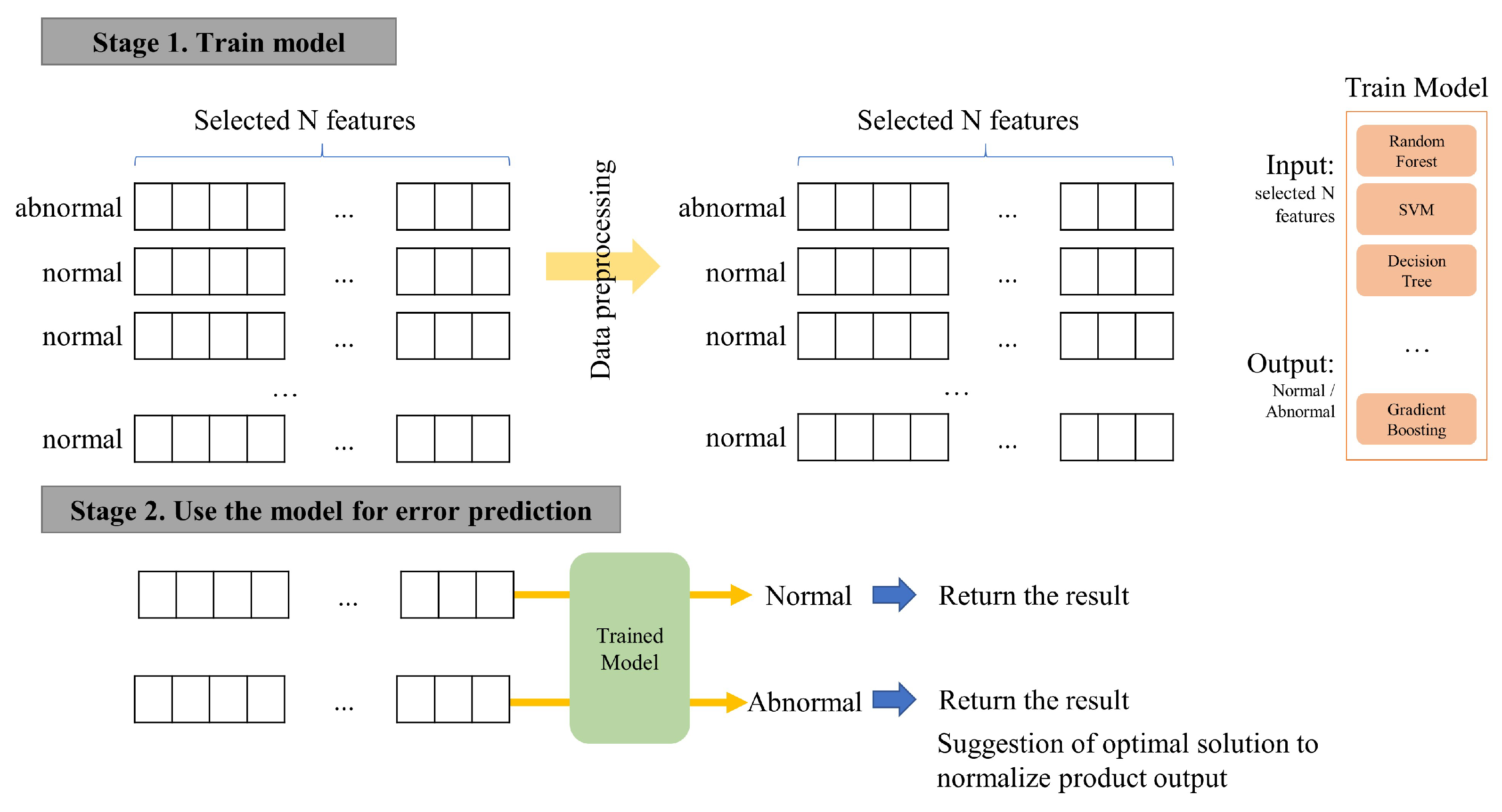
Quality assessment of products manufactured by this injection equipment was conducted through visual inspection, as shown in Figure 3, followed by manual entry into the kiosk. Through data analysis of quality-impacting factors and elements, it is imperative to identify the factors contributing to defects in injection quality and to enhance the accuracy of defect detection and reduce the error rate by utilizing machine learning models. The total number of data used was 18,668, of which 70% was allocated to the training set, 15% to the validation set, and 15% to the test set. The training set was utilized to train all the data, after which the model demonstrating the best results based on the validation set was selected. The final accuracy was calculated using the test set to derive the optimal solution. The overall workflow is illustrated in Figure 4 below.

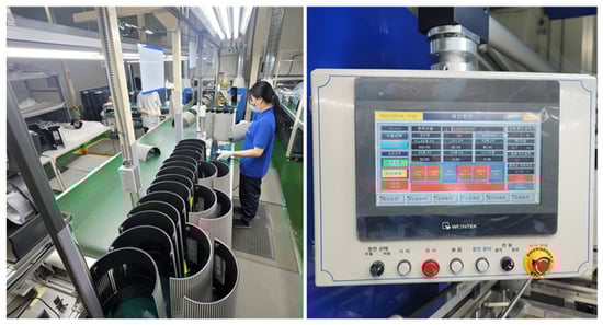
Figure 3. Quality inspection method for the product.

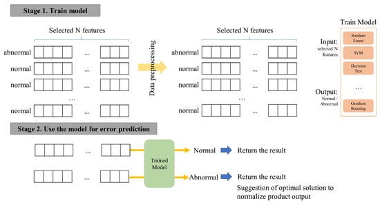
Figure 4. Overall flow of anomaly detection and optimal solution proposal for features capable of normalizing anomalous data.

3.1. Data Preprocessing

The initial step of the analysis focused on analyzing the features influencing the quality of the product. Upon examining the uniqueness of data per feature, it was observed that the majority possessed singular values. Furthermore, numerous features encompassed irrelevant information such as date details, a high proportion of missing values, and redundant entries. Since such inconsequential features adversely affect the accuracy of the model, a filtering process was undertaken to select 14 pertinent features, which are detailed in Table 1.

Table 1. Mean, max, min, and standard deviation for each feature used as input data.

	Mean	Max	Min	Std
P1_Max	184.4	253.1	0.3	14.5
P2_Max	326.4	400.3	0.2	20.7
Cycle Time	49.8	100	0	6.2
Actual Barrel Temperature HN	202,2	257.9	0	21.7
Actual Barrel Temperature H1	207.9	230.3	0	21.4
Actual Barrel Temperature H2	213.1	230.3	0	21.9
Actual Barrel Temperature H3	222.6	225.8	0	22.9
Actual Barrel Temperature H4	217.5	221.6	0	22.4
Actual Barrel Temperature H5	207.6	212.1	0	21.4
Filling Time	0.9	6.1	0	0.1
Metering Time	17.1	41.8	0	2.5
Max Injection Pressure	93.2	132.2	0	10.5
Max Injection Velocity	107.4	118.2	0	11.1
Cooling Time	18.1	32	0	2.1

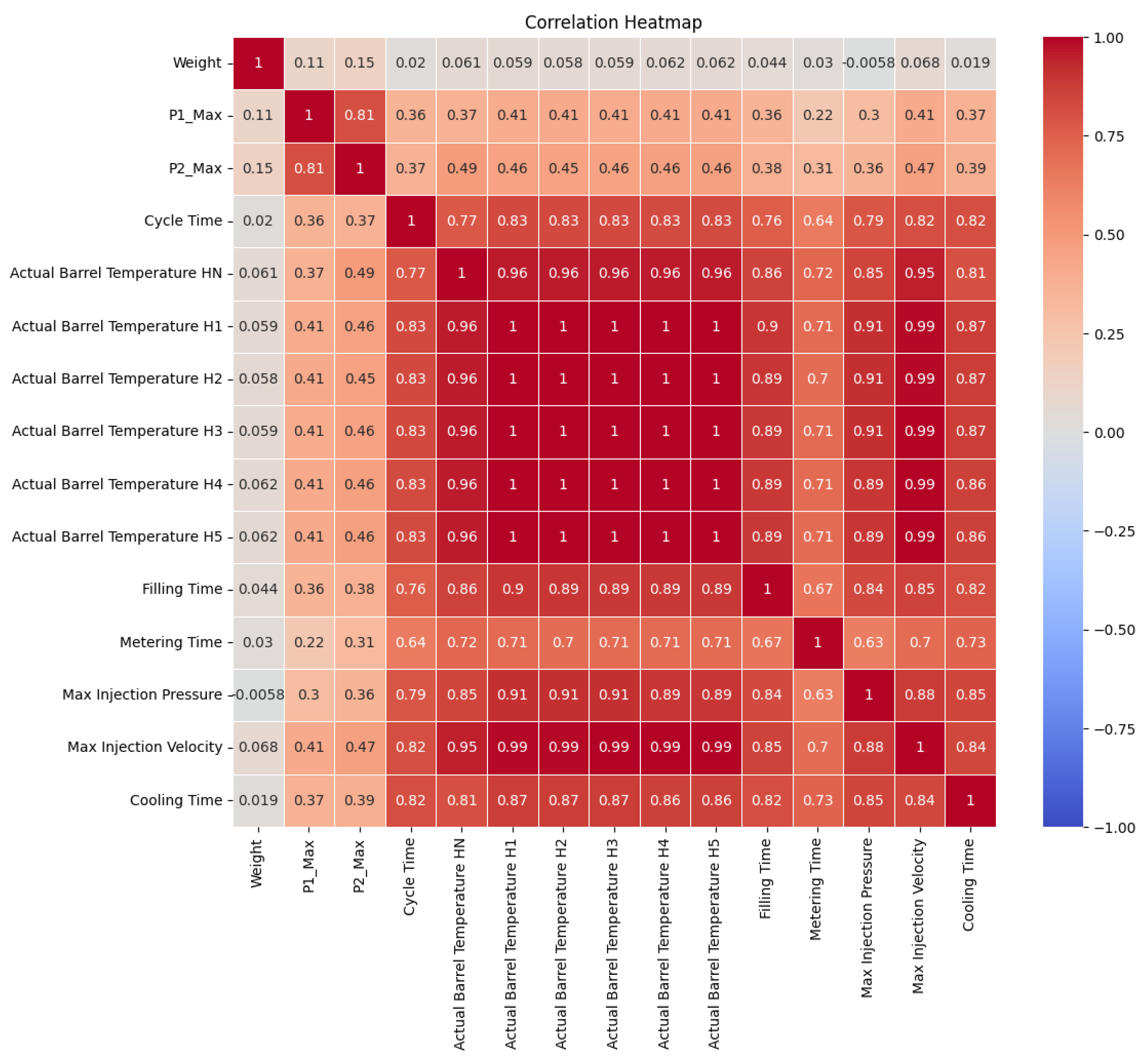
Additionally, the distinction between normal and abnormal products was based on the product’s weight, with the weight range of 450 to 650 kg being indicative of normal products and any deviation from this range representing abnormal data. A correlation analysis was conducted for each of the 14 chosen features and the weight. Figure 5 below shows the correlation between each feature.

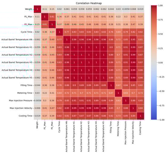
Figure 5. Correlation analysis of selected features.

The subsequent step involved labeling the data as normal or abnormal to address the problem of predicting product quality as a binary classification issue using the weight range. An examination of the total dataset revealed 18,124 entries as normal and 959 as defective, representing a significant imbalance at a ratio of approximately 19:1. We used the Synthetic Minority Oversampling Technique (SMOTE) [29,30] to solve this imbalance problem. SMOTE generates new synthetic samples by utilizing the differences between the data points of the minority class, proving more effective than simple duplication in oversampling scenarios. Finally, to solve the problem that the scale of each feature may have different influence on model learning, all feature values were normalized to fall within the 0 to 1 range [31].

3.2. Anomaly Detection Using Machine Learning Models

Model training ensued next. To predict product defects using data collected from the factory that had undergone preprocessing, a total of five machine learning-based classification models were utilized: K-Nearest Neighbors Classifier, Decision Trees Classifier, Random Forest Classifier, Extra Trees Classifier, and Gradient Boosting Classifier. In employing each model, parameters such as the number of neighbors (n_neighbors), the number of trees (n_estimators), the maximum depth of the trees (max_depth), and the learning rate (learning_rate) were meticulously controlled to ensure a fair comparison of accuracy across models [32,33,34,35,36]. Furthermore, the Grid Search method was employed to identify the most optimal combination of parameters for each model [37]. Grid Search performs 5-fold cross-validation over all combinations within a predefined grid of parameters, selecting the combination that best fits the model [38]. By appropriately adjusting these parameters, the complexity of the models was constrained, and the risk of overfitting was minimized. The remaining parameters of the model were kept at default values. Table 2 shows the optimal hyperparameters for each model found through Grid Search.

Table 2. Best parameters determined by Grid Search.

Model	Parameters
	n_neighbors	n_estimators	max_depth	learning_rate
K Neighbors Classifier	5	-	-	-
Decision Tree Classifier	-	-	11	-
Random Forest Classifier	-	20	13	-
Extra Trees Classifier	-	15	17	-
Gradient Boosting Classifier	-	25	11	0.1

Following the training of all models, performance evaluation on the validation and test datasets was conducted. The metrics used for performance evaluation were Accuracy, Precision, Recall, and F1 Score [39]. Through the evaluation of each model’s performance, the most suitable classification algorithm for anomaly detection was identified.

3.3. Finding the Optimal Solution for Abnormal Data

Rather than merely determining whether the product is normal or abnormal, we analyzed which features contribute to the classification of data as abnormal and subsequently proposed methods for optimizing these features to normalize abnormal data. This process was carried out using the Gradient Boosting Classifier, which exhibited the best performance. In this study, three methods were employed to identify the features with the most significant influence on the model’s predictions and to propose optimal solutions for normalizing values based on the selected features. The following provides detailed explanations of each method.

3.3.1. SHAP

The primary method employed was the utilization of Tree SHAP. This technique was applied to extract and analyze the feature importance, which holds a crucial role in the model’s predictive decisions. Specifically, SHAP values were calculated for each data sample classified as defective, enabling a quantitative assessment of the magnitude and direction of each feature’s influence on the model’s predictions. Through this approach, the top three features exerting the most substantial influence on the predictive decisions for each sample were identified. By adjusting the values of the selected features to the average values of those features in the normal data, optimal values for these features were proposed. This adjustment of each feature’s influence provided insights into how such changes could affect the model’s predictions.

3.3.2. Optimal Solution Presentation Using Mode

The paramount objective of XAI is to provide a logical explanation to users regarding the derivation of a model’s outcomes. It elucidates the predictions of models that are otherwise perceived as black boxes and plays a crucial role in enhancing the user’s trust in the outcomes of the trained models. However, in the context of proposing optimal solutions based on SHAP, the explanations may not be user-friendly for non-experts. Moreover, the computational cost of calculating the contribution of each feature across all possible combinations to find the optimal solution can be significant, potentially rendering it unsuitable for real-time factory environments. Consequently, we propose an alternative XAI technique that is applicable to tree-based machine learning models. In the manufacturing process, the quantity of data available for training neural-based deep learning models is often insufficient, leading to frequent instances of models not fitting the data adequately. Hence, anomaly detection issues are often resolved using machine learning-based approaches, with multi-tree-based models frequently demonstrating superior performance. In our task, the multi-tree-based Gradient Boosting model exhibited the highest performance in anomaly detection. Multi-tree-based models incorporate conditional statements in each tree node, with each condition having the characteristics of an if-else statement for a single feature [40].

We posited that the high frequency of features which appear in the node conditions would have a more significant influence on decision making, and we selected the top N features of abnormal data based on frequency. Subsequently, it was converted to the median value of features in all normal data and presented as the optimal solution. Pseudocode that succinctly describes the process of deriving the optimal solution using the second method is shown in Algorithm 1.

Algorithm 1 Correct Features Based on Frequency

Require:   $model$: A multi-tree-based machine learning model Require:   $normal\_data$: Dataset containing normal instances Require:   N: Number of top features to consider Ensure:   $corrected\_features$: Feature vector with corrected values   1: Initialize empty dictionary $feature\_frequency$   2: for each $tree$ in $model$.trees() do   3:     for each $node$ in $tree$ do   4:           Extract feature from node’s condition   5:           Increment count in $feature\_frequency$   6:     end for   7: end for   8: Determine top N features with highest frequency   9: Initialize $corrected\_features$ with input features   10: for each top N feature do   11:       Calculate average value in $normal\_data$   12:       Calculate difference with feature’s value in $corrected\_features$   13:       Correct feature value in $corrected\_features$   14: end for   15: return   $corrected\_features$

3.3.3. Optimization Using Conditions on Nodes

In this study, another proposed method also based on multi-tree-based models. As with other methods, if the predicted result from the tree-based model is abnormal data, it is predicted through various conditional statements in the node. This method places more focus on these conditions. In reality, the range of features in normal data exhibits a certain degree of variability around the median value. Therefore, in order to normalize outlier data effectively, it is necessary to adjust the feature values within an acceptable range rather than changing them to the median value. Taking this into consideration, we utilized the node conditions of the tree-based model as the optimal solution for normalizing outlier data. We acquired the condition values of all final prediction nodes in the multi-tree model, arranged the values to be changed in descending order of the difference between the input instance’s feature values and the condition values, and then fed them back into the model to verify normalization. If normalization is achieved, the process is stopped, and the proposed features and modified values are returned. Algorithm 2 is a pseudocode that succinctly outlines this process.

Algorithm 2 Adjust Features for Normalization

Require:   $model$: A multi-tree-based machine learning model Require:   $input\_features$: Vector of input features Ensure:   $adjusted\_features$: Adjusted feature vector   1: $adjusted\_features\leftarrow input\_features$   2: while $model.predict(adjusted\_features)$ is ’abnormal’ do   3:       Initialize an empty list $feature\_differences$   4:       for each $tree$ in $model.trees\left(\right)$ do   5:             Determine the final node for $adjusted\_features$   6:             Extract condition and threshold at the final node   7:             Calculate difference between $adjusted\_features$ and threshold   8:             Add feature index and difference to $feature\_differences$   9:       end for   10:     Sort $feature\_differences$ in descending order of differences   11:     Select feature with largest difference   12:     Adjust this feature in $adjusted\_features$   13: end while   14: return   $adjusted\_features$

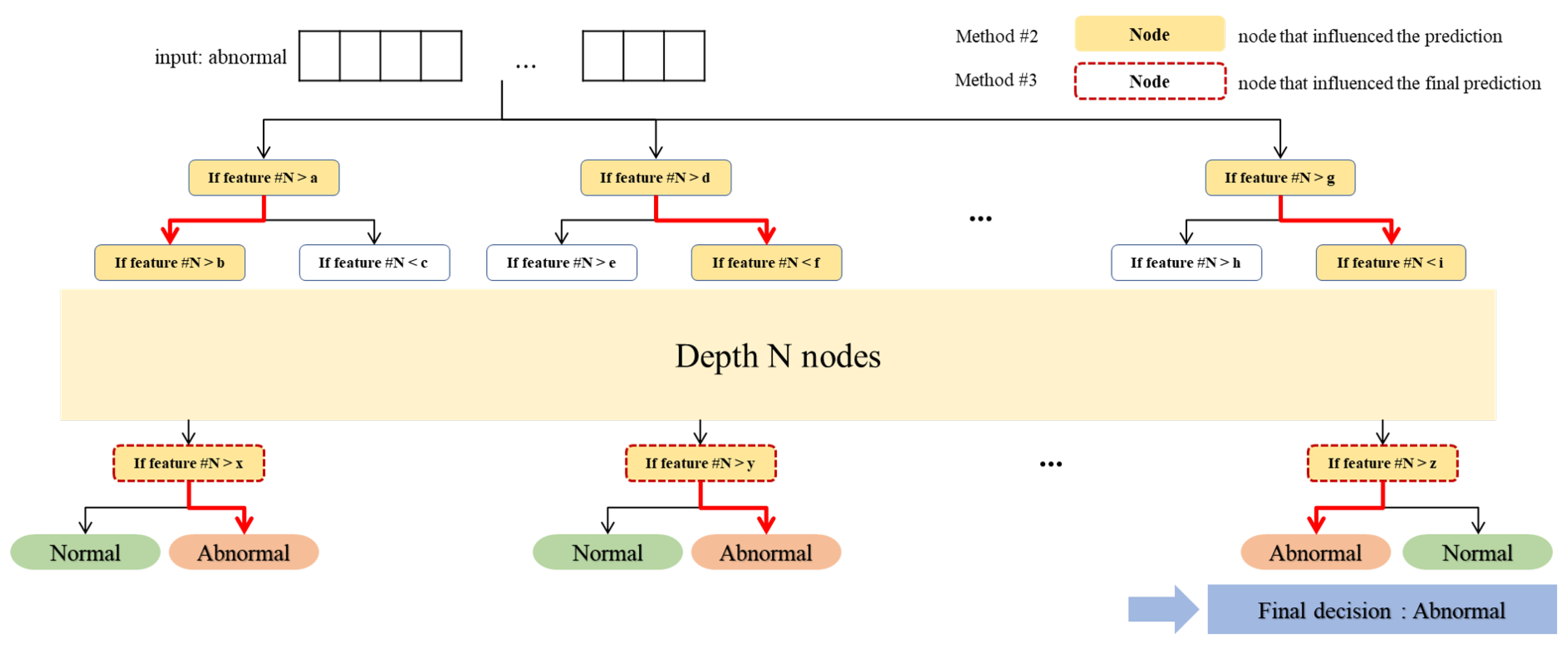
This method presents the advantage of offering a reasonable magnitude of change when proposing optimal solutions for features. It continuously attempts to adjust values until the model’s prediction is normalized, thereby ensuring a higher rate of successful normalization. Overall, we performed XAI in Methods #2 and #3 by analyzing the predictions of the tree-based model from two perspectives: features that frequently appeared in the predictions and features that were involved in the final prediction. The meaning of each is shown in Figure 6.

Figure 6. Example images to illustrate the nodes that influenced the prediction.

4. Results

The prediction results for each model are presented in Table 3 and Figure 7. We conducted anomaly detection using a variety of machine learning-based models, with unified data preprocessing and conditions for each model.

Table 3. The results of the performance evaluation.

Model	Accuracy	Precision	Recall	F1 Score
K-Nearest Neighbors Classifier	82.94%	0.8869	0.7551	0.8157
Decision Tree Classifier	85.88%	0.9110	0.7952	0.8492
Random Forest Classifier	90.73%	0.9724	0.8384	0.9004
Extra Trees Classifier	82.50%	0.8970	0.7343	0.8075
Gradient Boosting Classifier	94.80%	0.9851	0.9097	0.9459

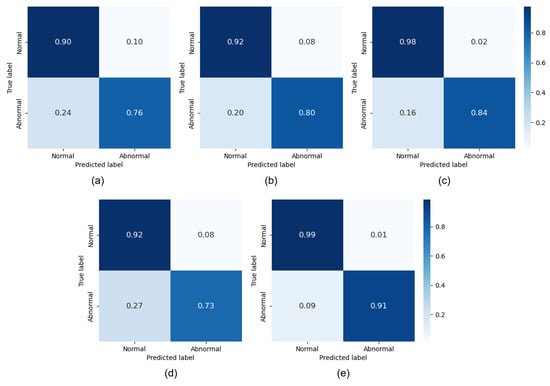
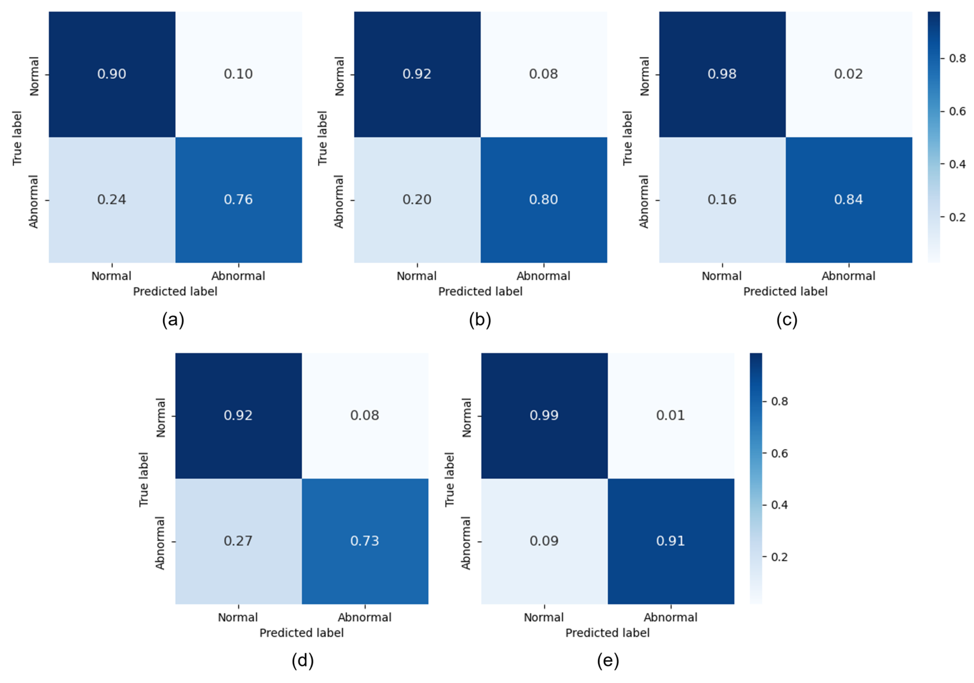
Figure 7. Results of confusion matrix for each model: (a) K-Nearest Neighbors Classifier; (b) Decision Tree Classifier; (c) Random Forest Classifier; (d) Extra Trees Classifier; (e) Gradient Boosting Classifier.

As can be observed from Table 3, the data indicate that the Gradient Boosting Classifier demonstrated the highest performance. We proceeded with the anomaly data normalization using the Gradient Boosting Classifier. Table 4 below presents the normalization rates for each of the three proposed methods.

Table 4. Results of normalization ratio for Gradient Boosting Classifier.

Method	Explanation	Rate of Anomaly Data Normalization
Method #1	SHAP + feature mean	97.30%
Method #2	Most frequent feature + feature mean	97.30%
Method #3	Last node feature + last node condition	100.00%

Among of our dataset, there were 111 outliers, and it was observed that when the third method was employed, all data previously predicted as outliers were successfully normalized. Furthermore, with the first method, 108 out of the 111 defective data points were normalized, and with the second method, 107 were normalized. These results confirm that over 97% of the data was effectively normalized in both instances.

5. Discussion

In the Results section above, it was observed that the normalization ratios for Method #1 and Method #2 are the same from Table 3. For further analysis, we also analyzed the actual outputs from real input data to see which features each method suggests to normalize and by how much. Table 5 displays examples of the suggested change features and values for each method.

Table 5. Examples of requested change features and amount for normalization for each method.

Sample	Method	Feature	Value
Sample 1	Method #1	P2_Max	−20.2260
		Max Injection Pressure	3.1238
		Max Injection Velocity	0.1854
	Method #2	P2_Max	−20.2260
		Max Injection Pressure	3.1238
		Cycle Time	0.8976
	Method #3	Cycle Time	20.2875
		Metering Time	5.5550
		Max Injection Pressure	3.4275
Sample 2	Method #1	P2_Max	−19.5260
		Max Injection Pressure	3.2238
		Actual Barrel Temperature H5	−0.0064
	Method #2	P2_Max	−19.5260
		Max Injection Pressure	3.2238
		Cycle Time	1.0976
	Method #3	Cycle Time	20.4895
		Max Injection Pressure	3.5285
		-	-

It is noteworthy that both Method #1 and Method #2 point to similar features and suggest the same value of change in both samples. Also, in the case of Method #3, the recommended change values for the overlapping feature ‘Max Injection Pressure’ were similar in size at 3.1238 and 3.4275, even though they were derived in a different way from Method #1 and Method #2, and in the case of sample 2, the suggested change values for `Max Injection Pressure’ were similar in size at 3.2238 and 3.5285, as well. By comparing the correction values for the different methods on a real-world example, we found that the features and ranges of the corrections provided by each method were similar. This means that when our three methods actually encounter outlier data, we can be confident that the feature is indeed significant in determining that it is an outlier because the correction ranges are similar. In addition to Gradient Boosting, we also performed normalization of the Random Forest model. The normalization ratio for Random Forest is shown in Table 6.

Table 6. Results of normalization ratio for Random Forest Classifier.

Method	Explanation	Rate of Anomaly Data Normalization
Method #1	SHAP + feature mean	99.32%
Method #2	Most frequent feature + feature mean	86.59%
Method #3	Last node feature + last node condition	80.49%

As can be seen in Table 6, it is difficult to expect normalization performance with Method #3 when the model’s inherent performance is not high. Methods #1 and #2 rely on the model’s characteristics to detect relevant features within anomalous data, but they employ values from normal data when it comes to adjustments for normalization. However, Method #3 employs the model not only for feature detection but also for normalization adjustments, thus producing outcomes more closely tied to the model’s architecture. Since the model’s own accuracy is not high, the rate of normalization is also a result derived from the model. Therefore, it is not necessarily indicative of a performance decline. Upon reviewing the results, it can be confirmed that the methods which most deeply reflect the model’s characteristics have a higher dependency on the model’s accuracy.

6. Conclusions

In this study, we conducted research that not only facilitates anomaly detection but also provides explanations and improvement measures for the predicted results, which can be more effectively utilized when using artificial intelligence-based models in actual manufacturing settings. It was ascertained that to render the explanation of prediction results more significant, the accuracy of the model itself must first be ensured. Through experiments, we refined our data in various ways and secured accuracy to achieve sufficiently reliable anomaly detection outcomes. Subsequently, we acquired features with high impact on the model’s predictions using three different methods. These included a method utilizing SHAP and two methods exploiting the intrinsic characteristics of tree-based models. Furthermore, we presented strategies for how much correction of the influential features is appropriate for normalizing instances predicted as abnormal. Indeed, we applied our three proposed methods to the factory data and observed that the normalization rate of outlier data exceeded 95% for all methods, with total normalization achieved when the last method was applied. Moving forward, we aim to conduct future research in two directions. Firstly, we plan to apply our methods to other factory data not utilized in this study to validate their effectiveness across diverse datasets. Additionally, we intend to apply our methodology to multivariate time-series data and develop anomaly detection methodologies that consider temporal pattern changes. This will be particularly helpful in precisely detecting complex anomalies that can occur in dynamic manufacturing processes.

References

- Maklin, S. The Ultimate Guide to Plastic Injection Moulding Cost. Available online: https://medium.com/@maklin.si/the-ultimate-guide-to-plastic-injection-moulding-cost-fdf3e5c14760 (accessed on 2 March 2024).
- Mr, A.B.; Humbe, D.M.K. Optimization of Critical Processing Parameters Forplastic Injection Molding of Polypropylene for Enhancedproductivity and Reduced Time for New Productdevelopment. Int. J. Mech. Eng. Technol. (IJMET) 2013, 5, 108–115. [Google Scholar]
- Sofianidis, G.; Rožanec, J.M.; Mladenic, D.; Kyriazis, D. A review of explainable artificial intelligence in manufacturing. arXiv 2021, arXiv:2107.02295. [Google Scholar]
- Sheuly, S.S.; Ahmed, M.U.; Begum, S.; Osbakk, M. Explainable machine learning to improve assembly line automation. In Proceedings of the 2021 4th International Conference on Artificial Intelligence for Industries (AI4I), Laguna Hills, CA, USA, 20–22 September 2021; pp. 81–85. [Google Scholar]
- Wang, Y.; Bai, X.; Liu, C.; Tan, J. A multi-source data feature fusion and expert knowledge integration approach on lithium-ion battery anomaly detection. J. Electrochem. Energy Convers. Storage 2022, 19, 021003. [Google Scholar]
- Yeh, C.C.M.; Zhu, Y.; Dau, H.A.; Darvishzadeh, A.; Noskov, M.; Keogh, E. Online amnestic dtw to allow real-time golden batch monitoring. In Proceedings of the 25th ACM SIGKDD International Conference on Knowledge Discovery & Data Mining, Anchorage, AK, USA, 4–8 August 2019; pp. 2604–2612. [Google Scholar]
- Paul, K.C.; Schweizer, L.; Zhao, T.; Chen, C.; Wang, Y. Series AC arc fault detection using decision tree-based machine learning algorithm and raw current. In Proceedings of the 2022 IEEE Energy Conversion Congress and Exposition (ECCE), Detroit, MI, USA, 9–13 October 2022; pp. 1–8. [Google Scholar]
- Kariri, E.; Louati, H.; Louati, A.; Masmoudi, F. Exploring the advancements and future research directions of artificial neural networks: A text mining approach. Appl. Sci. 2023, 13, 3186. [Google Scholar] [CrossRef]
- Gupta, A.K.; Sharma, R.; Ojha, R.P. Video anomaly detection with spatio-temporal inspired deep neural networks (DNN). In Proceedings of the 2023 6th International Conference on Contemporary Computing and Informatics (IC3I), Uttar Pradesh, India, 14–16 September 2023; Volume 6, pp. 1112–1118. [Google Scholar]
- Fang, C.; Wang, Q.; Huang, B. A Machine Learning Approach for Anomaly Detection in Power Mixing Equipment Intelligent Bearing Fault Diagnosis. In Proceedings of the 2023 IEEE 3rd International Conference on Power, Electronics and Computer Applications (ICPECA), Shenyang, China, 29–31 January 2023; pp. 912–919. [Google Scholar]
- Li, D.; Liu, Z.; Armaghani, D.J.; Xiao, P.; Zhou, J. Novel ensemble tree solution for rockburst prediction using deep forest. Mathematics 2022, 10, 787. [Google Scholar] [CrossRef]
- Aghaabbasi, M.; Ali, M.; Jasiński, M.; Leonowicz, Z.; Novák, T. On hyperparameter optimization of machine learning methods using a Bayesian optimization algorithm to predict work travel mode choice. IEEE Access 2023, 11, 19762–19774. [Google Scholar]
- Kramer, O.; Kramer, O. K-nearest neighbors. In Dimensionality Reduction with Unsupervised Nearest Neighbors; Springer: Berlin/Heidelberg, Germany, 2013; pp. 13–23. [Google Scholar]
- Dinata, R.K.; Adek, R.T.; Hasdyna, N.; Retno, S. K-nearest neighbor classifier optimization using purity. In Proceedings of the AIP Conference Proceedings; AIP Publishing: Lhokseumawe, Aceh, Indonesia, 2023; Volume 2431. [Google Scholar]
- Quinlan, J.R. Induction of decision trees. Mach. Learn. 1986, 1, 81–106. [Google Scholar]
- Colledani, D.; Anselmi, P.; Robusto, E. Machine learning-decision tree classifiers in psychiatric assessment: An application to the diagnosis of major depressive disorder. Psychiatry Res. 2023, 322, 115127. [Google Scholar] [CrossRef]
- Breiman, L. Random forests. Mach. Learn. 2001, 45, 5–32. [Google Scholar] [CrossRef]
- Shaheed, K.; Szczuko, P.; Abbas, Q.; Hussain, A.; Albathan, M. Computer-aided diagnosis of COVID-19 from chest x-ray images using hybrid-features and random forest classifier. Healthcare 2023, 11, 837. [Google Scholar] [CrossRef]
- Geurts, P.; Ernst, D.; Wehenkel, L. Extremely randomized trees. Mach. Learn. 2006, 63, 3–42. [Google Scholar] [CrossRef]
- Pagliaro, A. Forecasting Significant Stock Market Price Changes Using Machine Learning: Extra Trees Classifier Leads. Electronics 2023, 12, 4551. [Google Scholar] [CrossRef]
- Friedman, J.H. Greedy function approximation: A gradient boosting machine. Ann. Stat. 2001, 29, 1189–1232. [Google Scholar] [CrossRef]
- Torky, M.; Gad, I.; Hassanien, A.E. Explainable AI model for recognizing financial crisis roots based on Pigeon optimization and gradient boosting model. Int. J. Comput. Intell. Syst. 2023, 16, 50. [Google Scholar] [CrossRef]
- Lundberg, S.; Lee, S.I. A Unified Approach to Interpreting Model Predictions. arXiv 2017, arXiv:1705.07874. [Google Scholar]
- Hassija, V.; Chamola, V.; Mahapatra, A.; Singal, A.; Goel, D.; Huang, K.; Scardapane, S.; Spinelli, I.; Mahmud, M.; Hussain, A. Interpreting black-box models: A review on explainable artificial intelligence. Cogn. Comput. 2024, 16, 45–74. [Google Scholar] [CrossRef]
- Mariotti, E.; Sivaprasad, A.; Moral, J.M.A. Beyond prediction similarity: ShapGAP for evaluating faithful surrogate models in XAI. In Proceedings of the World Conference on Explainable Artificial Intelligence, Lisbon, Portugal, 26–28 July 2023; pp. 160–173. [Google Scholar]
- Lundberg, S.M.; Erion, G.G.; Lee, S.I. Consistent individualized feature attribution for tree ensembles. arXiv 2018, arXiv:1802.03888. [Google Scholar]
- Celik, S.; Logsdon, B.; Lee, S.I. Efficient dimensionality reduction for high-dimensional network estimation. In Proceedings of the International Conference on Machine Learning, Beijing, China, 22–24 June 2014; pp. 1953–1961. [Google Scholar]
- Chen, T.; Guestrin, C. Xgboost: A scalable tree boosting system. In Proceedings of the 22nd ACM SIGKDD International Conference on Knowledge Discovery and Data Mining, San Francisco, CA, USA, 13–17 August 2016; pp. 785–794. [Google Scholar]
- Chawla, N.V.; Bowyer, K.W.; Hall, L.O.; Kegelmeyer, W.P. SMOTE: Synthetic minority over-sampling technique. J. Artif. Intell. Res. 2002, 16, 321–357. [Google Scholar] [CrossRef]
- Joloudari, J.H.; Marefat, A.; Nematollahi, M.A.; Oyelere, S.S.; Hussain, S. Effective class-imbalance learning based on SMOTE and convolutional neural networks. Appl. Sci. 2023, 13, 4006. [Google Scholar] [CrossRef]
- Umar, M.A.; Chen, Z.; Shuaib, K.; Liu, Y. Effects of feature selection and normalization on network intrusion detection. Authorea Prepr. 2024. [Google Scholar] [CrossRef]
- Inyang, U.G.; Ijebu, F.F.; Osang, F.B.; Afolorunso, A.A.; Udoh, S.S.; Eyoh, I.J. A Dataset-Driven Parameter Tuning Approach for Enhanced K-Nearest Neighbour Algorithm Performance. Int. J. Adv. Sci. Eng. Inf. Technol. 2023, 13, 380–391. [Google Scholar] [CrossRef]
- Patange, A.D.; Pardeshi, S.S.; Jegadeeshwaran, R.; Zarkar, A.; Verma, K. Augmentation of decision tree model through hyper-parameters tuning for monitoring of cutting tool faults based on vibration signatures. J. Vib. Eng. Technol. 2023, 11, 3759–3777. [Google Scholar] [CrossRef]
- Yang, D.; Xu, P.; Zaman, A.; Alomayri, T.; Houda, M.; Alaskar, A.; Javed, M.F. Compressive strength prediction of concrete blended with carbon nanotubes using gene expression programming and random forest: Hyper-tuning and optimization. J. Mater. Res. Technol. 2023, 24, 7198–7218. [Google Scholar] [CrossRef]
- Talukder, M.S.H.; Akter, S. An improved ensemble model of hyper parameter tuned ML algorithms for fetal health prediction. Int. J. Inf. Technol. 2024, 16, 1831–1840. [Google Scholar] [CrossRef]
- Abbas, M.A.; Al-Mudhafar, W.J.; Wood, D.A. Improving permeability prediction in carbonate reservoirs through gradient boosting hyperparameter tuning. Earth Sci. Inform. 2023, 16, 3417–3432. [Google Scholar] [CrossRef]
- Shekar, B.; Dagnew, G. Grid search-based hyperparameter tuning and classification of microarray cancer data. In Proceedings of the 2019 Second International Conference on Advanced Computational and Communication Paradigms (ICACCP), Gangtok, India, 25–28 February 2019; pp. 1–8. [Google Scholar]
- Zhang, X.; Liu, C.A. Model averaging prediction by K-fold cross-validation. J. Econom. 2023, 235, 280–301. [Google Scholar] [CrossRef]
- Du, S.; Wang, K.; Cao, Z. Bpr-net: Balancing precision and recall for infrared small target detection. IEEE Trans. Geosci. Remote Sens. 2023, 61, 1–15. [Google Scholar] [CrossRef]
- Zhang, C.; Zhang, Y.; Shi, X.; Almpanidis, G.; Fan, G.; Shen, X. On incremental learning for gradient boosting decision trees. Neural Process. Lett. 2019, 50, 957–987. [Google Scholar] [CrossRef]
Disclaimer/Publisher’s Note: The statements, opinions and data contained in all publications are solely those of the individual author(s) and contributor(s) and not of MDPI and/or the editor(s). MDPI and/or the editor(s) disclaim responsibility for any injury to people or property resulting from any ideas, methods, instructions or products referred to in the content. |
© 2024 by the authors. Licensee MDPI, Basel, Switzerland. This article is an open access article distributed under the terms and conditions of the Creative Commons Attribution (CC BY) license (https://creativecommons.org/licenses/by/4.0/).