Adaptive PI Controller for Speed Control of Electric Drives Based on Model Reference Adaptive Identification

Abstract

In this paper, to achieve auto-setting of PI controller gains when mechanical parameters are unknown, two adaptive PI controllers for speed control of electric drives are developed based on model reference adaptive identification. The adaptive linear neuron (ADALINE) neural network is used to interpret the proposed adaptive PI controller. The effect of the low-pass filter used for the feedback speed and the Coulomb friction torque on parameter identification is analysed, and a new motion equation using filtered speed is given. Additionally, a parameter identification method based on unipolar speed reference is provided. The two proposed adaptive PI controllers and the conventional PI controller are compared based on the high-precision digital simulation using MATLAB/Simulink (version R2023a). The simulation results show that both of the two proposed adaptive PI controllers are able to identify mechanical parameters, but the adaptive PI-1 controller outperforms the adaptive PI-2 controller due to its better noise attenuation performance.

1. Introduction

Precision control of electric drives is inherently challenging due to the diverse sources of disturbances and uncertainties, as highlighted in [1]. The classical Proportional-Integral-Derivative (PID) controller, characterized by a one-degree-of-freedom structure, faces difficulties in simultaneously achieving optimal tracking performance and effective disturbance rejection. This limitation underscores the complexity of realizing decoupled control for both tracking performance and disturbance rejection properties [2]. Hence, several advanced control algorithms characterized by a two-degree-of-freedom (TDOF) structure have been proposed. Notably, TDOF PID control [3], disturbance observer-based control (DOBC) [4,5], and active disturbance rejection control (ADRC) [6,7,8] stand out as extensively investigated methodologies among various TDOF control algorithms.

Recently, generalized active disturbance rejection control (GADRC) [9] using generalized proportional integral control (GPIC) and generalized proportional integral observer (GPIO) was developed based on the differential flatness theory. Compared with the conventional ADRC, GADRC performs better either in disturbance rejection property for low-frequency disturbances or in suppression performance for high-frequency measurement noise [10,11,12], and thus is attracting more attention in research on electric drives. Motivated by one of the original ideas in ADRC [13,14], i.e., establishing a direct connection between the classical PID control and other modern control techniques [15,16], the relationship between GADRC and generalized PID control was analysed in [17]. It was found that the GADRC can be interpreted as the generalized PID with low-pass filters or the so-called TDOF generalized PID. However, compared with generalized PID, GADRC is easier to implement since the GPIC and GPIO has specific physical interpretation. In GADRC, the PI regulator in GPIC and the one in GPIO can be designed based on the same principle because of the duality between GPIC and GPIO. Therefore, the key in designing the GADRC is to design the PI regulator. Though GADRC with offline tuned gains can provide good control performance if the motor parameters are known. However, the system parameters may gradually change after a long running time, degrading the control performance if the gains are not updated [18]. To improve the system’s robustness to parameter variations, adaptive PI regulators are usually employed.

In [18,19,20,21,22], several adaptive controllers were designed with different principles, such as adaptive gain PID based on the supervisory gradient method [18], adaptive compensating feedback control [20], and model reference adaptive control (MRAC) based on adaptive compensating feedforward control [21,22]. It should be noted that whether the adaptive gain or the compensation term need to be trained before application. However, how to train the adaptive term is not explained in the above references. In [23], accurate mechanical parameters are identified in an adaptive PI observer using the excitation signal of a unipolar sinusoidal speed reference. Nevertheless, the speed tracking error is not considered. In [24], the PI controller was designed based on adaptive control method and a neural network is used for interpreting the essence of the integrator. However, only disturbance torque variation is considered.

In this paper, two adaptive PI controllers considering the variations of the mechanical parameters, including moment of inertia, viscous friction torque coefficient, and disturbance torque, are developed using the same principle in [23,24]. The adaptive linear neuron (ADALINE) neural network [25,26] is employed to interpret the developed adaptive PI controllers. The effect of the two practical issues: the low-pass filter used for feedback speed and the Coulomb friction torque, are investigated on parameter identification methods. A modified motion equation considering these two practical issues is introduced and the relationship between the identified parameters and their actual values are clarified. Additionally, a parameter identification method based on unipolar speed reference is provided.

The rest of this article is organized as follows. Section 2 introduces the mathematical model of the mechanical system and the conventional PI controller for the speed control system. Section 3 presents the proposed adaptive PI controller and two practical issues in real applications. Simulation results and the analysis are shown in Section 4. Finally, the conclusions are drawn in Section 5.

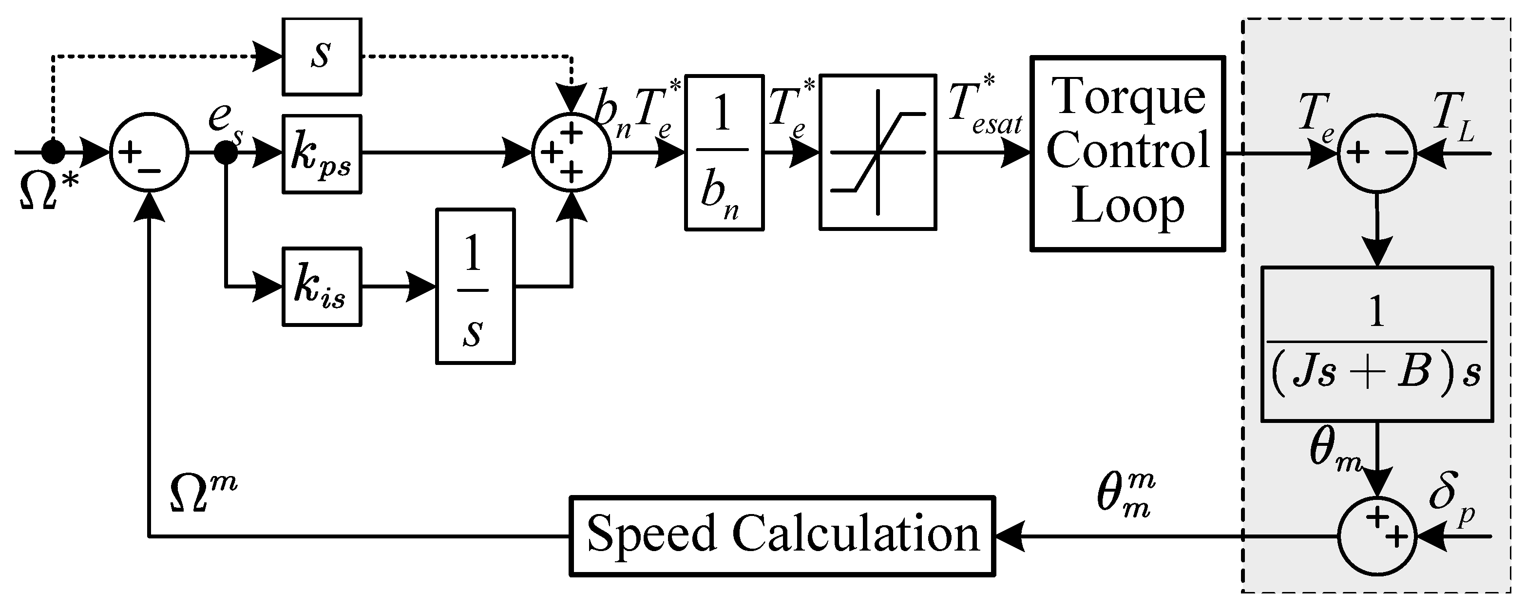
2. Conventional PI Controller for Speed Control

2.1. Mathematical Model of the Speed Control System

The feedback control law is formulated with the aim of effectively mitigating the speed reference tracking error. Following the feedback control law, the control output, specifically the torque reference, can be derived. Consequently, it is imperative to represent the system model as a function of the torque references.

$$\dot{\Omega }=\frac{-B\Omega +T_e-T_L}{J}=b(T_e^{*}-T_n)=b{T}_e^{*}+d_n$$

(1)

where $\Omega$ represents the mechanical angular velocity, $T_e$ and $T_e^{*}$ denote the electromagnetic torque and its reference, B stands for the viscous friction torque coefficient, $T_L$ signifies the load torque, b is defined as $1/J$ (the control gain), and $T_n$ is the disturbance torque resulting from the torque tracking error, load torque, and viscous friction torque, expressed as $T_n=T_e^{*}-T_e+B\Omega +T_L$, with $d_n$ representing the disturbance caused by the lumped disturbance torque and defined as $-T_n/J$.

Considering uncertainties in the moment of inertia J, control systems often employ the nominal value $J_n$. Introducing $b_n=1/J_n$ as the nominal control gain, the system model can be adjusted as follows:

$$\dot{\Omega }=b{T}_e^{*}+d_n=b_n{T}_e^{*}-(b_n-b)T_e^{*}+d_n=b_n{T}_e^{*}+d_{to}$$

(2)

where $d_{to}=d_n+(b-b_n)T_e^{*}$ is the total disturbance when considering the inertia mismatches.

2.2. Design of the Conventional PI Controller

The speed reference can be denoted as ${\Omega }^{*}$, then the speed tracking error can be expressed as $e_s={\Omega }^{*}-\Omega$, and we have

$${\dot{e}}_s={\dot{\Omega }}^{*}-\dot{\Omega }={\dot{\Omega }}^{*}-b_n{T}_e^{*}-d_{to}$$

(3)

When using proportional control, the desired speed tracking error convergence law is designed as:

$${\dot{e}}_s=-k_{ps}{e}_s$$

(4)

where $k_{ps}$ is the proportional gain.

Substituting (4) into (3) yields:

$$T_e^{*}=\frac{{\dot{\Omega }}^{*}+k_{ps}\left({\Omega }^{*}-\Omega \right)-d_{to}}{b_n}$$

(5)

When the total disturbance $d_{to}$ in (5) is substituted by its estimated value ${\widehat{d}}_{to}$, the torque reference can be modified as:

$$T_e^{*}=\frac{{\dot{\Omega }}^{*}+k_{ps}{e}_s-{\widehat{d}}_{to}}{b_n}$$

(6)

Using the torque reference expressed by (6), the state equation of the speed tracking error (3) is modified as:

$$\begin{array}{c}\hfill {\dot{e}}_s={\dot{\Omega }}^{*}-\dot{\Omega }={\dot{\Omega }}^{*}-b_n{T}_e^{*}-d_{to}=-k_{ps}{e}_s-{\tilde{d}}_{to}\end{array}$$

(7)

where ${\tilde{d}}_{to}=d_{to}-{\widehat{d}}_{to}$ is the total disturbance estimation error.

Adopting the adaptive design method in [24], the torque reference using PI controller can be expressed as:

$$T_e^{*}=\frac{{\dot{\Omega }}^{*}+k_{ps}{e}_s+k_{is}\int e_{s}dt}{b_n}$$

(8)

The block diagram of the conventional PI controller is shown in Figure 1.

Figure 1. Block diagram of conventional PI control system.

2.3. Dynamic Performance of the Speed PI Control System

In real applications, the measured speed as ${\Omega }^m$ is used for feedback, and thus the actual torque reference is modified as:

$$\begin{array}{cc}\hfill T_e^{*}\left(s\right)& =\frac{s{\Omega }^{*}\left(s\right)+\left(k_{ps}+\frac{k_{is}}{s}\right)\left[{\Omega }^{*}\left(s\right)-{\Omega }^m\left(s\right)\right]}{b_n} \hfill \\ \hfill & =\frac{s{\Omega }^m\left(s\right)+\left(s+k_{ps}+\frac{k_{is}}{s}\right)\left[{\Omega }^{*}\left(s\right)-{\Omega }^m\left(s\right)\right]}{b_n}\hfill \end{array}$$

(9)

According to (1), the relationship between the torque reference and the nominal disturbance can be expressed by:

$$T_e^{*}\left(s\right)=\frac{s\Omega \left(s\right)-d_n\left(s\right)}{b}=\frac{s{\Omega }^m\left(s\right)-\left[d_n\left(s\right)+s{\delta }_n\left(s\right)\right]}{b}$$

(10)

Substituting (9) into (10), the system output can be deduced as:

$${\Omega }^m\left(s\right)=\frac{s^2+k_{ps}s+k_{is}}{k_b{s}^2+k_{ps}s+k_{is}}{\Omega }^{*}\left(s\right)+\frac{k_{b}s}{k_b{s}^2+k_{ps}s+k_{is}}\left[d_n\left(s\right)+s{\delta }_n\left(s\right)\right]$$

(11)

where $k_b=b_n/b=J/J_n$ is the control gain ratio.

When the moment of inertia is known, i.e., $k_b=J/J_n=1$, the system has an ideal tracking performance under no disturbance and the characteristic polynomial is usually set as $s^2+k_{ps}s+k_{is}={(s+{\omega }_c)}^2$, where ${\omega }_c$ is the bandwidth of the speed control loop. The two gains in PI controller can be calculated by $k_{ps}=2{\omega }_c$ and $k_{is}={\omega }_c^2$. However, when the moment of inertia is unknown or it varies with operating conditions, $k_b\ne 1$, the system dynamic performance will degrade. When expressing the characteristic polynomial of the closed-loop control system as $k_b{s}^2+k_{ps}s+k_{is}=k_b(s^2+2{\zeta }_1{\omega }_{c1}s+{\omega }_{c1}^2)$, the actual damping ratio ${\zeta }_1$ and the actual natural frequency ${\omega }_{c1}$ can be determined using the following equations:

$${\zeta }_1=\frac{\zeta }{\sqrt{k_b}},{\omega }_{c1}=\frac{{\omega }_c}{\sqrt{k_b}}$$

(12)

It can be observed that both the actual damping ratio ${\zeta }_1$ and the actual natural frequency ${\omega }_{c1}$ decreases as $k_b$ increases, resulting in a higher overshoot in the step response as well as a slower dynamic performance. To solve this problem, an adaptive PI controller is developed in this paper.

3. Adaptive PI Controller for Speed Control Based on MRAI

3.1. Adaptive PI Controller Considering Mechanical Parameters Uncertainties

The motion Equation (1) can also be expressed as:

$$\dot{\Omega }=\left(T_e-T_L-B\Omega \right)/J=(T_e^{*}-T_d-B\Omega )/J$$

(13)

where $T_d=T_e^{*}-T_e+T_L$ consists of the disturbance caused by the load torque and the torque tracking error.

The state equation of the speed tracking error can be expressed as:

$${\dot{e}}_s={\dot{\Omega }}^{*}-\dot{\Omega }={\dot{\Omega }}^{*}-\left(T_e^{*}-T_d-B\Omega \right)/J$$

(14)

Therefore, the ideal torque reference when using proportional control can also be deduced as:

$$T_e^{*}=J\left({\dot{\Omega }}^{*}+k_{ps}{e}_s\right)+B\Omega +T_d$$

(15)

Denote the estimated values of J, B, and $T_d$ as $\widehat{J}$, $\widehat{B}$ and ${\widehat{T}}_d$, the actual torque reference can be expressed as:

$${\widehat{T}}_e^{*}=\widehat{J}\left({\dot{\Omega }}^{*}+k_{ps}{e}_s\right)+\widehat{B}\Omega +{\widehat{T}}_d$$

(16)

Substituting (16) into (3) yields:

$$\begin{array}{cc}\hfill {\dot{e}}_s& ={\dot{\Omega }}^{*}-\dot{\Omega } \hfill \\ \hfill & ={\dot{\Omega }}^{*}-\frac{\widehat{J}\left({\dot{\Omega }}^{*}+k_{ps}{e}_s\right)+\widehat{B}\Omega +{\widehat{T}}_d-T_d-B\Omega }{J} \hfill \\ \hfill & =-\frac{\widehat{J}}{J}{k}_{ps}{e}_s-\frac{\tilde{J}{\dot{\Omega }}^{*}+\tilde{B}\Omega +{\tilde{T}}_d}{J} \hfill \end{array}$$

(17)

where $\tilde{J}=\widehat{J}-J$, $\tilde{B}=\widehat{B}-B$, and ${\tilde{T}}_d={\widehat{T}}_d-T_d$ are the estimation error of inertia, viscous friction coefficient, and disturbance torque, respectively.

According to [27], the Lyapunov function can be selected as:

$$V=\frac{1}{2}{e}_s^2+\frac{{\tilde{J}}^2}{2J{k}_J}+\frac{{\tilde{B}}^2}{2J{k}_B}+\frac{{\tilde{T}}_d^2}{2J{k}_d}$$

(18)

where $k_J$, $k_B$, and $k_d$ are the adaptive gain for estimating the inertia, viscous friction coefficient, and disturbance torque.

The derivative of the Lyapunov function (18) can be obtained as follows:

$$\begin{array}{cc}\hfill \dot{V}& =e_s{\dot{e}}_s+\frac{1}{J{k}_J}\tilde{J}\dot{\tilde{J}}+\frac{1}{J{k}_B}\tilde{B}\dot{\tilde{B}}+\frac{1}{J{k}_d}{\tilde{T}}_d{\dot{\tilde{T}}}_d \hfill \\ \hfill & =-\frac{\widehat{J}}{J}{k}_{ps}{e}_s^2-\frac{\tilde{J}{\dot{\Omega }}^{*}+\tilde{B}\Omega +{\tilde{T}}_d}{J}{e}_s+\frac{1}{J{k}_J}\tilde{J}\dot{\tilde{J}}+\frac{1}{J{k}_B}\tilde{B}\dot{\tilde{B}}+\frac{1}{J{k}_d}{\tilde{T}}_d{\dot{\tilde{T}}}_d \hfill \\ \hfill & =-\frac{\widehat{J}}{J}{k}_{ps}{e}_s^2+\frac{1}{J}\left[\frac{\tilde{J}}{k_J}\left(\dot{\tilde{J}}-k_J{\dot{\Omega }}^{*}{e}_s\right)+\frac{\tilde{B}}{k_B}\left(\dot{\tilde{B}}-k_B\Omega e_s\right)+\frac{{\tilde{T}}_d}{k_d}\left({\dot{\tilde{T}}}_d-k_d{e}_s\right)\right]\hfill \end{array}$$

(19)

The stability of the system can be ensured by equating the second term on the right-hand side of Equation (19) to zero, i.e.,

$$\left\{\begin{array}{c}\dot{\tilde{J}}=\dot{\widehat{J}}-\dot{J}=k_J{\dot{\Omega }}^{*}{e}_s\\ \dot{\tilde{B}}=\dot{\widehat{B}}-\dot{B}=k_B\Omega e_s\\ {\dot{\tilde{T}}}_d={\dot{\widehat{T}}}_d-{\dot{T}}_d=k_d{e}_s\end{array}\right.$$

(20)

Assuming constant values for the actual inertia, viscous friction coefficient, and disturbance torque, the adaptive law governing the estimation of these three parameters can be formulated as follows:

$$\left\{\begin{array}{c}\widehat{J}\left(t\right)=k_J\int {\dot{\Omega }}^{*}{e}_{s}dt+\widehat{J}\left(0\right)\hfill \\ \widehat{B}\left(t\right)=k_B\int \Omega e_{s}dt+\widehat{B}\left(0\right)\hfill \\ {\widehat{T}}_d\left(t\right)=k_d\int e_{s}dt+{\widehat{T}}_d\left(0\right)\hfill \end{array}\right.$$

(21)

where $\widehat{J}\left(0\right)$, $\widehat{B}\left(0\right)$, and ${\widehat{T}}_d\left(0\right)$ are the initial values.

If we rewrite (17) as:

$${\dot{e}}_s=-k_{ps}{e}_s-\frac{\tilde{J}({\dot{\Omega }}^{*}+k_{ps}{e}_s)+\tilde{B}\Omega +{\tilde{T}}_d}{J}$$

(22)

then the adaptive law expressed by (21) becomes:

$$\left\{\begin{array}{c}\widehat{J}\left(t\right)=k_J\int ({\dot{\Omega }}^{*}+k_{ps}{e}_s)e_{s}dt+\widehat{J}\left(0\right)\hfill \\ \widehat{B}\left(t\right)=k_B\int \Omega e_{s}dt+\widehat{B}\left(0\right) \hfill \\ {\widehat{T}}_d\left(t\right)=k_d\int e_{s}dt+{\widehat{T}}_d\left(0\right) \hfill \end{array}\right.$$

(23)

According to (16), (21), and (23), the block diagram of the two adaptive PI controllers are shown in Figure 2. Here, the two adaptive PI controllers are noted as adaptive PI-1 and adaptive PI-2. It can be seen that the only difference between the two adaptive PI controllers is the input of the inertia estimators.

Figure 2. Block diagram of adaptive PI control system. (a) Adaptive PI-1. (b) Adaptive PI-2.

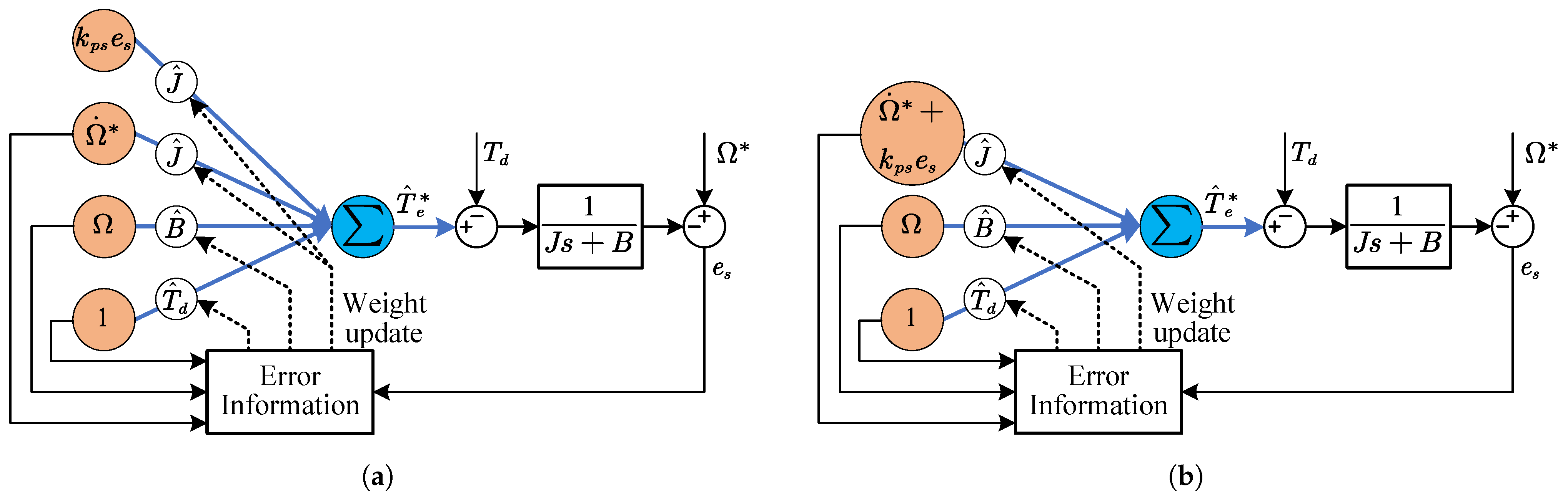
3.2. Interpretation of Adaptive PI Controller Using ADALINE

The torque reference expressed by (15) and (16) can also be rewritten as:

$$T_e^{*}=\left[\begin{array}{ccc}J& B& T_d\end{array}\right]\left[\begin{array}{c}{\dot{\Omega }}^{*}\\ \Omega \\ 1\end{array}\right]+J{k}_{ps}{e}_s={\mathit{w}}^{\mathrm{T}}\mathit{h}+J{k}_{ps}{e}_s$$

(24)

$${\widehat{T}}_e^{*}=\left[\begin{array}{ccc}\widehat{J}& \widehat{B}& {\widehat{T}}_d\end{array}\right]\left[\begin{array}{c}{\dot{\Omega }}^{*}\\ \Omega \\ 1\end{array}\right]+\widehat{J}{k}_{ps}{e}_s={\widehat{\mathit{w}}}^{\mathbf{T}}\mathit{h}+\widehat{J}{k}_{ps}{e}_s$$

(25)

where $\mathit{w}$ and $\widehat{\mathit{w}}$ are the weight vector and its estimated value, respectively, while $\mathit{h}$ is the input vector of the ADALINE.

$$\mathit{w}=\left[\begin{array}{c}J\\ B\\ T_d\end{array}\right],\widehat{\mathit{w}}=\left[\begin{array}{c}\widehat{J}\\ \widehat{B}\\ {\widehat{T}}_d\end{array}\right],\mathit{h}=\left[\begin{array}{c}{\dot{\Omega }}^{*}\\ \Omega \\ 1\end{array}\right]$$

According to (24), there is

$$B\Omega +T_d={\mathit{w}}^{\mathrm{T}}\mathit{h}-J{\dot{\Omega }}^{*}$$

(26)

The derivative of the speed tracking error can be obtained as:

$$\begin{array}{cc}\hfill {\dot{e}}_s& ={\dot{\Omega }}^{*}-\dot{\Omega } \hfill \\ \hfill & ={\dot{\Omega }}^{*}-\frac{{\widehat{T}}_e^{*}-B\Omega -T_d}{J} \hfill \\ \hfill & ={\dot{\Omega }}^{*}-\frac{{\widehat{\mathit{w}}}^{\mathrm{T}}\mathit{h}+\widehat{J}{k}_{ps}{e}_s+J{\dot{\Omega }}^{*}-{\mathit{w}}^{\mathrm{T}}\mathit{h}}{J} \hfill \\ \hfill & =-\frac{\widehat{J}}{J}{k}_{ps}{e}_s-\frac{{\tilde{\mathit{w}}}^{\mathrm{T}}\mathit{h}}{J} \hfill \end{array}$$

(27)

Similarly, the Lyapunov function can be selected as:

$$V=\frac{1}{2}{e}_s^2+\frac{1}{2J}{\tilde{\mathit{w}}}^{\mathrm{T}}{\mathit{k}}_{\mathit{w}}^{-1}\tilde{\mathit{w}}$$

(28)

where ${\mathit{k}}_{\mathit{w}}^{-1}$ is a gain matrix.

The derivative of (28) can be calculated as:

$$\begin{array}{cc}\hfill \dot{V}& =e_s{\dot{e}}_s+\frac{{\tilde{\mathit{w}}}^{\mathrm{T}}{\mathit{k}}_{\mathit{w}}^{-1}\dot{\tilde{\mathit{w}}}}{J} \hfill \\ \hfill & =-\frac{\widehat{J}}{J}{k}_{ps}{e}_s^2-\frac{{\tilde{\mathit{w}}}^{\mathrm{T}}\mathit{h}}{J}{e}_s+\frac{{\tilde{\mathit{w}}}^{\mathrm{T}}{\mathit{k}}_{\mathit{w}}^{-1}\dot{\tilde{\mathit{w}}}}{J} \hfill \\ \hfill & =-\frac{\widehat{J}}{J}{k}_{ps}{e}_s^2-\frac{{\tilde{\mathit{w}}}^{\mathrm{T}}{\mathit{k}}_{\mathit{w}}^{-1}}{J}\left(\dot{\tilde{\mathit{w}}}-{\mathit{k}}_{\mathit{w}}\mathit{h}{e}_s\right)\hfill \end{array}$$

(29)

The system appears to be stable if the second item on the right-hand side of the equation is set to zero, i.e.,

$$\dot{\tilde{\mathit{w}}}=\dot{\widehat{\mathit{w}}}-\dot{\mathit{w}}={\mathit{k}}_{\mathit{w}}\mathit{h}{e}_s$$

(30)

Under the assumption of $\dot{\mathit{w}}=0$, the adaptive law governing the weight vector can be articulated as follows:

$$\widehat{\mathit{w}}=\int {\mathit{k}}_{\mathit{w}}\mathit{h}{e}_{s}dt$$

(31)

By setting ${\mathit{k}}_{\mathit{w}}$ as:

$${\mathit{k}}_{\mathit{w}}=\left[\begin{array}{ccc}{k}_J& 0& 0\\ 0& k_B& 0\\ 0& 0& k_d\end{array}\right]$$

the adaptive law can be obtained as:

$$\left[\begin{array}{c}\widehat{J}\left(t\right)\\ \widehat{B}\left(t\right)\\ {\widehat{T}}_d\left(t\right)\end{array}\right]=\int \left[\begin{array}{c}{k}_J{\dot{\Omega }}^{*}\\ k_B\Omega \\ k_d\end{array}\right]e_{s}dt+\left[\begin{array}{c}\widehat{J}\left(0\right)\\ \widehat{B}\left(0\right)\\ {\widehat{T}}_d\left(0\right)\end{array}\right]$$

(32)

If we modify $\mathit{h}$ in (24) and (25) as:

$$\mathit{h}=\left[\begin{array}{c}{\dot{\Omega }}^{*}+k_{ps}{e}_s\\ \Omega \\ 1\end{array}\right]$$

(33)

then (24) and (25) can be modified as $T_e^{*}={\mathit{w}}^{\mathrm{T}}\mathit{h}$ and ${\widehat{T}}_e^{*}={\widehat{\mathit{w}}}^{\mathrm{T}}\mathit{h}$, and the adaptive law expressed by (32) can be modified as:

$$\left[\begin{array}{c}\widehat{J}\left(t\right)\\ \widehat{B}\left(t\right)\\ {\widehat{T}}_d\left(t\right)\end{array}\right]=\int \left[\begin{array}{c}{k}_J\left({\dot{\Omega }}^{*}+k_{ps}{e}_s\right)\\ k_B\Omega \\ k_d\end{array}\right]e_{s}dt+\left[\begin{array}{c}\widehat{J}\left(0\right)\\ \widehat{B}\left(0\right)\\ {\widehat{T}}_d\left(0\right)\end{array}\right]$$

(34)

It can be seen that the adaptive law expressed by (32) and (34) are exactly the same as those expressed by (21) and (23). Figure 3 shows how the adaptive PI controller can be interpreted by ADALINE.

Figure 3. Interpretation of adaptive PI controller using ADALINE. (a) Adaptive PI-1. (b) Adaptive PI-2.

3.3. Practical Issues in Real Applications

In real applications, a LPF is usually used for attenuating the speed measurement noise and thus the feedback speed is the filtered speed ${\Omega }_f$. Assuming a first-order LPF with a time constant of $\tau$ is employed, the relationship between ${\Omega }_f$ and $\Omega$ can be expressed as:

$$\Omega =\tau {\dot{\Omega }}_f+{\Omega }_f$$

(35)

Using ${\Omega }_f$ as the output and considering the Coulomb friction torque coefficient $T_C$, the motion equation is modified as:

$$\begin{array}{cc}\hfill T_e^{*}& =J\dot{\Omega }+B\Omega +T_d+T_C\mathrm{sign}(\Omega ) \hfill \\ \hfill & =\left(J+B\tau \right){\dot{\Omega }}_f+J\tau {\ddot{\Omega }}_f+B{\Omega }_f+T_d+T_C\mathrm{sign}(\Omega )\hfill \end{array}$$

(36)

To obtain smoothed identified parameters, sinusoidal speed is usually employed as the persistent excitation signal. Assuming the sinusoidal speed has an angular frequency of ${\omega }_{PE}$, and it can be expressed as the sum of an AC component and DC component, i.e., ${\Omega }_f={\Omega }_{f\_ac}+{\Omega }_{f\_dc}$, there is ${\ddot{\Omega }}_f=-{\omega }_{PE}^2{\Omega }_f$.

If there is no offset in the speed, ${\Omega }_{f\_dc}=0$, then the Coulomb friction torque is an AC signal that in phase of the real speed $\Omega$, and thus it can be approximated by $T_C\mathrm{sign}(\Omega )\approx \Delta J·{\dot{\Omega }}_f+\Delta B·{\Omega }_f$, where $\Delta J$ and $\Delta B$ are the incremental inertia and incremental viscous friction torque coefficient, and they depends on $T_C$ and $\tau$. As a result, the motion equation can be rewritten as:

$$T_e^{*}=\left(J+B\tau +\Delta J\right){\dot{\Omega }}_{f\_ac}+\left(B-J\tau {\omega }_{PE}^2+\Delta B\right){\Omega }_{f\_ac}+T_d$$

(37)

If a large offset is added in the speed reference so that the speed becomes unipolar, then the Coulomb friction torque is a constant torque such that it can be treated as part of the load torque. The motion equation can be rewritten as:

$$T_e^{*}=\left(J+B\tau \right){\dot{\Omega }}_{f\_ac}+\left(B-J\tau {\omega }_{PE}^2\right){\Omega }_{f\_ac}+T_d+T_C+\left(B-J\tau {\omega }_{PE}^2\right){\Omega }_{f\_dc}$$

(38)

Denote $J_1$, $B_1$, and $T_{d1}$ as the equivalent values of inertia, viscous friction torque coefficient, and load torque, we can express the motion equation in a unified form as:

$$T_e^{*}=J_1{\dot{\Omega }}_{f\_ac}+B_1{\Omega }_{f\_ac}+T_{d1}$$

(39)

In the case of bipolar speed, $J_1$, $B_1$, and $T_{d1}$ are expressed as:

$$\left\{\begin{array}{c}{J}_1=J+B\tau +\Delta J \hfill \\ B_1=B-J\tau {\omega }_{PE}^2+\Delta B\hfill \\ T_{d1}=T_d \hfill \end{array}\right.$$

(40)

In the case of unipolar speed, $J_1$, $B_1$, and $T_{d1}$ are expressed as:

$$\left\{\begin{array}{c}{J}_1=J+B\tau \hfill \\ B_1=B-J\tau {\omega }_{PE}^2 \hfill \\ T_{d1}=T_d+T_C+B_1{\Omega }_{f\_dc}\hfill \end{array}\right.$$

(41)

Since a LPF is used for the measured speed, a same LPF should be used for the speed reference so that the actual speed can track the real speed reference. Denote the filtered speed reference as ${\Omega }_f^{*}$. When using the motion equation expressed by (39), the adaptive law for the identified parameters can be modified as:

$$\left\{\begin{array}{c}{e}_{sf}={\Omega }_f^{*}-{\Omega }_f \hfill \\ {\widehat{J}}_1\left(t\right)=k_J\int {\dot{\Omega }}^{*}{e}_{sf}dt+{\widehat{J}}_1\left(0\right) \hfill \\ {\widehat{B}}_1\left(t\right)=k_B\int {\Omega }_{f\_ac}{e}_{sf}dt+{\widehat{B}}_1\left(0\right) \hfill \\ {\widehat{T}}_{d1}\left(t\right)=k_d\int e_{sf}dt+{\widehat{T}}_{d1}\left(0\right) \hfill \end{array}\right.$$

(42)

$$\left\{\begin{array}{c}{e}_{sf}={\Omega }_f^{*}-{\Omega }_f \hfill \\ {\widehat{J}}_1\left(t\right)=k_J\int ({\dot{\Omega }}^{*}+k_{ps}{e}_{sf})e_{sf}dt+{\widehat{J}}_1\left(0\right) \hfill \\ {\widehat{B}}_1\left(t\right)=k_B\int {\Omega }_{f\_ac}{e}_{sf}dt+{\widehat{B}}_1\left(0\right) \hfill \\ {\widehat{T}}_{d1}\left(t\right)=k_d\int e_{sf}dt+{\widehat{T}}_{d1}\left(0\right) \hfill \end{array}\right.$$

(43)

where ${\widehat{J}}_1\left(0\right)$, ${\widehat{B}}_1\left(0\right)$, and ${\widehat{T}}_{d1}\left(0\right)$ are the initial values.

The block diagrams of the two practical adaptive PI control system are shown in Figure 4.

Figure 4. Block diagrams of the two practical adaptive PI control system. (a) Adaptive PI-1. (b) Adaptive PI-2.

4. Simulation Verification

In this section, a high-resolution digital simulation model is developed using MATLAB/Simulink (version R2023a) to assess the functionality of the proposed two adaptive PI controllers. Additionally, a comparative analysis is conducted between the proposed adaptive PI controllers and the conventional PI controller, elucidating their relative advantages.

4.1. System Setup

The block diagram of the speed control system using adaptive PI controller is shown in Figure 5. The specific parameters of the examined PMSM are listed in Table 1. In the simulations, an incremental encoder with a resolution of 2500 pulse per round (PPR) is utilized. The rotor field-oriented control (RFOC) strategy with $i_d=0$ and space vector pulse width modulation (SVPWM) is adopted. The DC bus voltage is established as 150 V. Both the sampling period and control period for current and speed control are set as 0.1 ms. Current control is executed through a Decoupled Proportional-Integral (PI) Controller, with a specified bandwidth of 2000 rad/s. The negligible delay in the torque control loop allows it to be disregarded within the speed control system. A current limit of 9 A is imposed, and speed calculation is performed using the classical frequency method. To mitigate measurement noise, a first-order Low-Pass Filter (LPF) with a time constant of 1 ms is employed.

Figure 5. Block diagram of the simulation system.

Table 1. Parameters of the examined PMSM.

Symbol	Quantity	Symbol	Quantity
Rated power $P_N$	1.0 (kW)	polePair numbers $p_n$	4
Rated voltage $U_N$	220 (V)	D axis inductance $L_d$	3.4 (mH)
Rated speed $n_N$	2500 (r/min)	Q axis inductance $L_q$	3.4 (mH)
Rated torque $T_N$	4.0 (Nm)	Torque constant $K_t$	0.71 (Nm/A)
Current limit $I_{smax}$	9 (A)	Coulomb friction torque $T_C$	0.1 (Nm)
Stator resistance $R_s$	1.18 (Ohm)	Motor system inertia J	2.35 ($\mathrm{g}·{\mathrm{m}}^2$)

In the simulation, $k_{ps}=400$ rad/s, $k_d=10$, $k_J=5\times {10}^{-6}$, $k_B=0.01$. Three control systems: the conventional PI controller, the adaptive PI controller without identifying ${\widehat{B}}_1$, and the adaptive PI controller identifying ${\widehat{B}}_1$, are tested. The simulation time is set as 5 s. At the time instant of 1 s, sinusoidal speed reference is given under no load and the adaptive PI control is enabled. At the time instant of 3 s, a load is stepped from 0 Nm to 2 Nm.

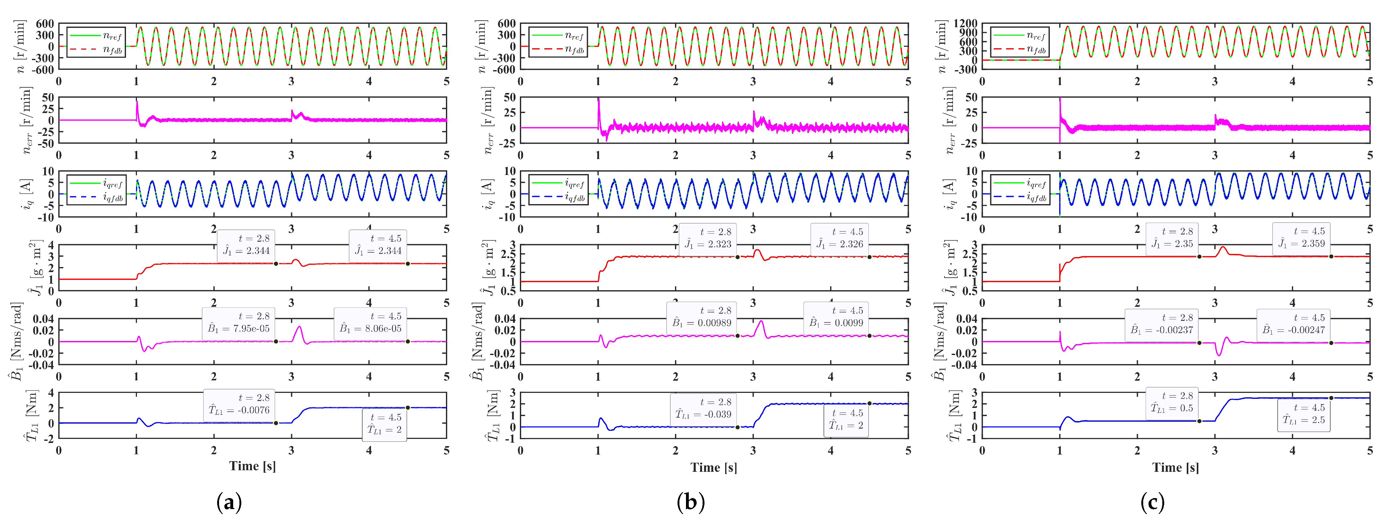
4.2. Simulation Verification of the Adaptive PI-1 Controller

The initial inertia is set as 1 $\mathrm{g}·{\mathrm{m}}^2$. When a bipolar sinusoidal speed reference expressed by $n_{ref}=500sin$(10 $\pi$t)r/min is employed, the simulation results of the three control systems without considering the Coulomb friction torque are shown in Figure 6. From Figure 6a, it can be seen that the conventional PI controller has a poor tracking performance due to the mismatched inertia. The identified load torque is oscillating because it is an integral of the speed tracking error, which is sinusoidal. In Figure 6b, the inertia is identified but the viscous friction torque coefficient is not. The oscillation in the identified load torque is greatly reduced, but not eliminated. Meanwhile, the identified inertia oscillates at the frequency of 10 Hz, which is twice of the frequency of the sinusoidal speed reference. The oscillation can be eliminated by identifying load torque, inertia and viscous friction torque coefficient simultaneously, as shown in Figure 6c. It can be seen that the actual inertia 2.35 $\mathrm{g}·{\mathrm{m}}^2$ can be identified, ${\widehat{B}}_1=-0.00237$ Nms/rad, which is very closed to $-J\tau {\omega }_{PE}^2=-0.00232$ Nms/rad, and the identified load torque levels at 2.8 s are −0.0005 Nm and 2 Nm, which are almost the same as the actual values. The error is caused by some unmodelled dynamics in the digital control system, such as the delay in sampling and control.

Figure 6. Simulation results under the sinusoidal speed reference without offset $n_{ref}=500sin\left(10\pi t\right)$ r/min when ${\widehat{J}}_1\left(0\right)=1\mathrm{g}·{\mathrm{m}}^2$ and $T_C=0$. (a) Conventional PI controller. (b) Adaptive PI-1 controller without identifying ${\widehat{B}}_1$. (c) Adaptive PI-1 controller identifying ${\widehat{B}}_1$.

When considering the Coulomb friction torque, simulation results of the adaptive PI controller will be affected. In Figure 7a,b, $T_C$ is 0.1 Nm and 0.5 Nm, respectively, the identified inertias are merely affected, they are 2.344 $\mathrm{g}·{\mathrm{m}}^2$ and 2.323 $g·{\mathrm{m}}^2$, however, the identified viscous friction torque coefficients are greatly affected, they become $8\times {10}^{-5}$ Nms/rad and $9.9\times {10}^{-3}$ Nms/rad. This is because the incremental inertia $\Delta J$ caused by the Coulomb friction torque is very small while the incremental viscous friction torque coefficient $\Delta B$ is large. The Coulomb friction torque causes the oscillation of the speed tracking error and thus leads to the oscillation of the identified parameters. To solve this problem, a unipolar speed reference expressed by $n_{ref}=500sin(10\pi t-\pi /2)+600$ r/min can be employed, as shown in Figure 7c.

Figure 7. Simulation results of the adaptive PI-1 controller under different $T_C$. (a) Bipolar speed reference and $T_C=0.1$ Nm. (b) Bipolar speed reference and $T_C=0.5$ Nm. (c) Unipolar speed reference and $T_C=0.5$ Nm.

To further verify the effectiveness of the proposed adaptive PI controller, the initial inertia is increased to 6 $\mathrm{g}·{\mathrm{m}}^2$ and the Coulomb friction torque coefficient $T_C$ is set as 0.1 Nm, simulation results are shown in Figure 8. Similarly, it can be seen that the conventional PI controller has a poor tracking performance, the speed tracking error can be greatly reduced by identifying inertia, but it cannot be eliminated if the viscous friction torque coefficient is not identified.

Figure 8. Simulation results under the sinusoidal speed reference with offset $n_{ref}=500sin(10\pi t-\pi /2)+600$ r/min when ${\widehat{J}}_1\left(0\right)=6 \mathrm{g}·{\mathrm{m}}^2$ and $T_C=0.1$ Nm. (a) Conventional PI controller. (b) Adaptive PI controller-1 without identifying ${\widehat{B}}_1$. (c) Adaptive PI-1 controller identifying ${\widehat{B}}_1$.

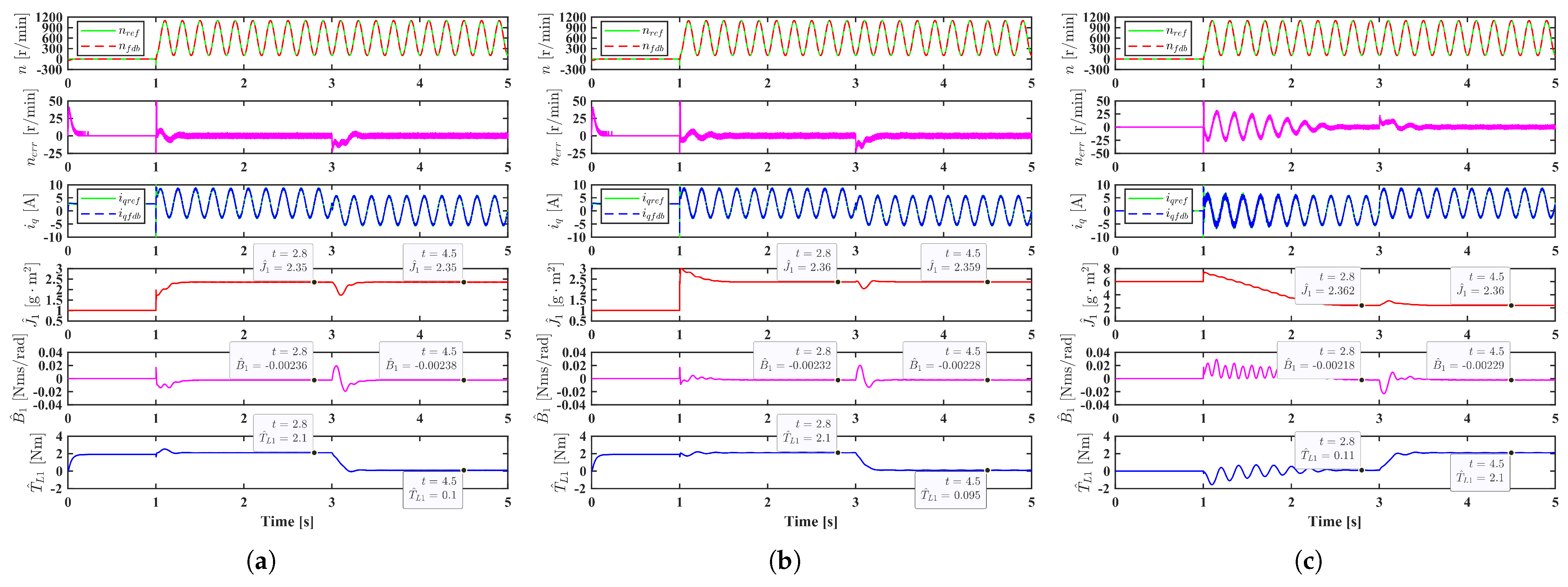
4.3. Comparison of the Adaptive PI-1 Controller and the Adaptive PI-2 Controller

When the initial inertia ${\widehat{J}}_1\left(0\right)$ and the Coulomb friction torque coefficient $T_C$ are set as 1 $\mathrm{g}·{\mathrm{m}}^2$ and 0.1 Nm, respectively, simulation results of the two adaptive PI controllers using the same gains are shown in Figure 9a,b, the zoomed-in views from the time 1 s to 3 s are shown in Figure 10. From the zoom views, it can be seen that the adaptive PI-2 controller has a larger oscillation in the identified parameters. The oscillation is caused by the larger noise introduced by the term “$k_{ps}{e}_{sf}$” in “${\dot{\Omega }}^{*}+k_{ps}{e}_{sf}$”. If we reduce the position measurement noise by setting the output format of the sampled position as “double”, the adaptive PI-2 controller can also has a good steady-state performance, as shown in Figure 9c and Figure 10c. These results shows that the adaptive PI-1 controller has better noise attenuation ability than the adaptive PI-2 controller.

Figure 9. Simulation results under the sinusoidal speed reference with offset $n_{ref}=500sin(10\pi t-\pi /2)+600$ r/min when ${\widehat{J}}_1\left(0\right)=1 \mathrm{g}·{\mathrm{m}}^2$ and $T_C=0.1$ Nm. (a) Adaptive PI-1 controller. (b) Adaptive PI-2 controller. (c) Adaptive PI-2 controller without position measurement noise.

Figure 10. Zoomed-in view of the simulation results in Figure 9 from 1 s to 3 s. (a) Adaptive PI-1 controller. (b) Adaptive PI-2 controller. (c) Adaptive PI-2 controller without position measurement noise.

Comparing the results shown in Figure 9a,c, it can be observed that the adaptive PI-2 controller has better dynamic performance than the adaptive PI-1 controller in the starting process, however it is slower when the load varies. From (42) and (43), it is known that the dynamic performance of the two controllers depends on the quantity of ${\dot{\Omega }}^{*}$ and ${\dot{\Omega }}^{*}+k_{ps}{e}_{sf}$. If we set load torque as 2 Nm from 0 s to 3 s and 0 Nm from 3 s to 5 s (the simulations results are shown in Figure 11a,b), it can be seen that the adaptive PI-2 controller has poorer dynamic performance than the adaptive PI-1 controller in the starting process, however it is faster when the load varies, which is quite opposite to the results in Figure 9. Similarly, when ${\widehat{J}}_1\left(0\right)=6 \mathrm{g}·{\mathrm{m}}^2$, by comparing Figure 11c with Figure 8c, it can be found that the adaptive PI-2 controller has poorer dynamic performance than the adaptive PI-1 controller whether in the starting process or in the load-changing process.

Figure 11. Simulation results when starting with 2Nm and unloading to 0 Nm at 3 s. (a) Adaptive PI-1 controller. (b) Adaptive PI-2 controller. (c) Adaptive PI-2 controller without position measurement noise.

From the above simulation results, it can be concluded that the adaptive PI-1 controller outperforms the adaptive PI-2 controller in real applications.

5. Conclusions

In this paper, to achieve auto-setting of PI controller gains when mechanical parameters are unknown, two adaptive PI controllers for speed control of electric drives are developed based on model reference adaptive identification. In real applications, the low-pass filter used for the feedback speed and the Coulomb friction torque has an effect on parameter identification. To address these two issues, a new motion equation using filtered speed is given, and the relationship between the identified parameters and their real values is studied. Additionally, a parameter identification method based on unipolar speed reference is provided. The only difference between the two adaptive PI controllers is the error information used for identifying the inertia. Simulation results show that the adaptive PI-1 controller is more practical due to its better noise attenuation performance.

It is worth pointing out that the principle of the adaptive PI controller is to divide the total disturbance torque into AC and DC components, the DC component disturbance is identified by the integral of the speed tracking error, whereas the AC component disturbance is identified by an ADALINE neural network, in which the feedback speed and its derivative are the basis, while the equivalent inertia and the equivalent viscous friction torque coefficient are two weights need to be trained. Therefore, the AC disturbance caused by other unmodelled dynamics can also be identified and compensated.

Torque ripple due to cogging torque or current harmonics is common in real-world applications, making the impractical assumption that the disturbance torque is constant. In the future, we plan to develop an adaptive PI controller that takes into account torque ripple. Furthermore, the adaptive control method utilised in this article requires a persistent excitation signal, which may not be permitted in some applications, such as robots and CNC machine tools. Adaptive methods for speed regulation systems without a persistent excitation signal remain an interesting topic.

References

- Yang, J.; Chen, W.H.; Li, S.; Guo, L.; Yan, Y. Disturbance/Uncertainty Estimation and Attenuation Techniques in PMSM Drives—A Survey. IEEE Trans. Ind. Electron. 2017, 64, 3273–3285. [Google Scholar] [CrossRef]
- Zuo, Y.; Chen, J.; Zhu, X.; Lee, C.H.T. Different Active Disturbance Rejection Controllers Based on the Same Order GPI Observer. IEEE Trans. Ind. Electron. 2022, 69, 10969–10983. [Google Scholar] [CrossRef]
- Harnefors, L.; Saarakkala, S.E.; Hinkkanen, M. Speed Control of Electrical Drives Using Classical Control Methods. IEEE Trans. Ind. Appl. 2013, 49, 889–898. [Google Scholar] [CrossRef]
- Chen, W.H.; Yang, J.; Guo, L.; Li, S. Disturbance-Observer-Based Control and Related Methods—An Overview. IEEE Trans. Ind. Electron. 2015, 63, 1083–1095. [Google Scholar] [CrossRef]
- Sariyildiz, E.; Oboe, R.; Ohnishi, K. Disturbance Observer-Based Robust Control and Its Applications: 35th Anniversary Overview. IEEE Trans. Ind. Electron. 2020, 67, 2042–2053. [Google Scholar] [CrossRef]
- Gao, Z. On the Centrality of Disturbance Rejection in Automatic Control. ISA Trans. 2014, 53, 850–857. [Google Scholar] [CrossRef] [PubMed]
- Liu, C.; Luo, G.; Duan, X.; Chen, Z.; Zhang, Z.; Qiu, C. Adaptive LADRC-based disturbance rejection method for electromechanical servo system. IEEE Trans. Ind. Appl. 2019, 56, 876–889. [Google Scholar] [CrossRef]
- Zhu, L.; Zhang, G.; Jing, R.; Bi, G.; Xiang, R.; Wang, G.; Xu, D. Nonlinear active disturbance rejection control strategy for permanent magnet synchronous motor drives. IEEE Trans. Energy Convers. 2022, 37, 2119–2129. [Google Scholar] [CrossRef]
- Sira-Ramírez, H.; Luviano-Juárez, A.; Ramírez-Neria, M.; Zurita-Bustamante, E.W. Active Disturbance Rejection Control of Dynamic Systems: A Flatness Based Approach; Butterworth-Heinemann: Oxford, UK, 2018. [Google Scholar]
- Zuo, Y.; Mei, J.; Jiang, C.; Yuan, X.; Xie, S.; Lee, C.H.T. Linear Active Disturbance Rejection Controllers for PMSM Speed Regulation System Considering the Speed Filter. IEEE Trans. Power Electron. 2021, 36, 14579–14592. [Google Scholar] [CrossRef]
- akomy, K.; Madonski, R. Cascade extended state observer for active disturbance rejection control applications under measurement noise. ISA Trans. 2021, 109, 1–10. [Google Scholar]
- Ahmad, S.; Ali, A. On active disturbance rejection control in presence of measurement noise. IEEE Trans. Ind. Electron. 2021, 69, 11600–11610. [Google Scholar] [CrossRef]
- Huang, Y.; Xue, W. Active Disturbance Rejection Control: Methodology and Theoretical Analysis. ISA Trans. 2014, 53, 963–976. [Google Scholar] [CrossRef]
- Feng, H.; Guo, B.Z. Active disturbance rejection control: Old and new results. Annu. Rev. Control 2017, 44, 238–248. [Google Scholar] [CrossRef]
- Xue, W.; Huang, Y. Comparison of the DOB Based Control, a Special Kind of PID Control and ADRC. In Proceedings of the 2011 American Control Conference, San Francisco, CA, USA, 29 June–1 July 2011; pp. 4373–4379. [Google Scholar]
- Zhong, S.; Huang, Y.; Guo, L. A Parameter Formula Connecting PID and ADRC. Sci. China Inf. Sci. 2020, 63, 192203. [Google Scholar] [CrossRef]
- Lin, P.; Wu, Z.; Fei, Z.; Sun, X.M. A Generalized PID Interpretation for High-Order LADRC and Cascade LADRC for Servo Systems. IEEE Trans. Ind. Electron. 2022, 69, 5207–5214. [Google Scholar] [CrossRef]
- Jung, J.W.; Leu, V.Q.; Do, T.D.; Kim, E.K.; Choi, H.H. Adaptive PID speed control design for permanent magnet synchronous motor drives. IEEE Trans. Power Electron. 2014, 30, 900–908. [Google Scholar] [CrossRef]
- Wang, Y.; Fang, S.; Hu, J. Active disturbance rejection control based on deep reinforcement learning of PMSM for more electric aircraft. IEEE Trans. Power Electron. 2022, 38, 406–416. [Google Scholar] [CrossRef]
- Kim, S.K.; Lee, K.G.; Lee, K.B. Singularity-free adaptive speed tracking control for uncertain permanent magnet synchronous motor. IEEE Trans. Power Electron. 2015, 31, 1692–1701. [Google Scholar] [CrossRef]
- Guo, L.; Parsa, L. Model reference adaptive control of five-phase IPM motors based on neural network. IEEE Trans. Ind. Electron. 2011, 59, 1500–1508. [Google Scholar] [CrossRef]
- Nguyen, A.T.; Rafaq, M.S.; Choi, H.H.; Jung, J.W. A model reference adaptive control based speed controller for a surface-mounted permanent magnet synchronous motor drive. IEEE Trans. Ind. Electron. 2018, 65, 9399–9409. [Google Scholar] [CrossRef]
- Zuo, Y.; Mei, J.; Zhang, X.; Lee, C.H.T. Simultaneous Identification of Multiple Mechanical Parameters in a Servo Drive System Using Only One Speed. IEEE Trans. Power Electron. 2021, 36, 716–726. [Google Scholar] [CrossRef]
- Zuo, Y.; Xie, S.; Cao, L.; Han, B.S.; Hoang, C.C.; You, C.; Chan, J.; Lee, C.H.T. A Novel Nonlinear Active Disturbance Rejection Controller for Speed Control of Electric Drives. In Proceedings of the 2022 IEEE Energy Conversion Congress and Exposition (ECCE), Detroit, MI, USA, 9–13 October 2022; pp. 1–5. [Google Scholar]
- Zhang, W. System identification based on a generalized ADALINE neural network. In Proceedings of the 2007 American Control Conference. IEEE, New York, NY, USA, 9–13 July 2007; pp. 4792–4797. [Google Scholar]
- Osorio-Arteaga, F.; Giraldo, E. Adaptive Neural Network Identification for Robust Multivariable Systems. IAENG Int. J. Appl. Math. 2024, 54, 68–76. [Google Scholar]
- Levine, W.S. The Control Handbook (Three Volume Set); CRC Press: Boca Raton, FL, USA, 2018. [Google Scholar]
Disclaimer/Publisher’s Note: The statements, opinions and data contained in all publications are solely those of the individual author(s) and contributor(s) and not of MDPI and/or the editor(s). MDPI and/or the editor(s) disclaim responsibility for any injury to people or property resulting from any ideas, methods, instructions or products referred to in the content. |
© 2024 by the authors. Licensee MDPI, Basel, Switzerland. This article is an open access article distributed under the terms and conditions of the Creative Commons Attribution (CC BY) license (https://creativecommons.org/licenses/by/4.0/).