Abstract
Industrial fans are critical components in industrial production, where unexpected damage of important fans can cause serious disruptions and economic costs. One trending market segment in this area is where companies are trying to add value to their products to detect faults and prevent breakdowns, hence saving repair costs before the main product is damaged. This research developed a methodology for early fault detection in a fan system utilizing machine learning techniques to monitor the operational states of the fan. The proposed system monitors the vibration of the fan using an accelerometer and utilizes a machine learning model to assess anomalies. Several of the most widely used algorithms for fault detection were evaluated and their results benchmarked for the vibration monitoring data. It was found that a simple Convolutional Neural Network (CNN) model demonstrated notable accuracy without the need for feature extraction, unlike conventional machine learning (ML)-based models. Additionally, the CNN model achieved optimal accuracy within 30 epochs, demonstrating its efficiency. Evaluating the CNN model performance on a validation dataset, the hyperparameters were updated until the optimal result was achieved. The trained model was then deployed on an embedded system to make real-time predictions. The deployed model demonstrated accuracy rates of 99.8%, 99.9% and 100.0% for Fan-Fault state, Fan-Off state, and Fan-On state, respectively, on the validation data set. Real-time testing further confirmed high accuracy scores ranging from 90% to 100% across all operational states. Challenges addressed in this research include algorithm selection, real-time deployment onto an embedded system, hyperparameter tuning, sensor integration, energy efficiency implementation and practical application considerations. The presented methodology showcases a promising approach for efficient and accurate fan fault detection with implications for broader applications in industrial and smart sensing applications.
1. Introduction
Industrial fans are critical components in industrial production, and unexpected damage of important fans can cause serious disruptions. These kinds of fans in general operate non-stop for long hours, and losing their functionality can have a high impact on the main equipment for which they provide ventilation. Incorrect or wrong assembly can cause breakdowns such as vibration, heating and making audible noise. Therefore, one of the trending markets segments is where companies are trying to add value to their product by introducing machine learning in such fan systems for early fault detection. This can help prevent major breakdowns resulting in long down times and save repair costs before the main product is damaged.
Machine learning techniques have been used in health monitoring of machines to assess anomaly fault detection [1] for more than a decade. These techniques can be simply explained as the process of learning historical data and making predictions about new sensor data. Artificial Intelligence (AI) and machine learning techniques have been researched for several decades, and their importance in Machine Health Monitoring applications has been increasing for the last 20 years [1]. Typically, these techniques have been implemented on powerful computers and/or microprocessors. However, implementing neural network (NN) solutions on low-power edge devices, namely the Arm Cortex-M microcontroller systems, has now became popular [1,2]. Microcontrollers, being compact embedded computing devices with minimal power requirements, offer a promising platform for introducing machine learning capabilities. Embedding machine learning on these microcontrollers enhances the performance of various daily-use devices, eliminating the need for expensive hardware installations or reliance on stable internet connections, which are often constrained by bandwidth, power limitations, and high latency [3].
This paper introduces an embedded machine learning approach for real-time fan fault detection. Leveraging the Application Software Pack from NXP, developers can implement neural networks on Microcontroller Unit (MCU)-based systems. This approach facilitates low-cost, low power consumption using smaller edge devices to empower smarter applications, decrease delay time, and save bandwidth. The following points encapsulate the key novelties that distinguish this work.
- Introduction of an Embedded Machine Learning Approach: Establishing the application of embedded machine learning for real-time anomalies detection.
- Development and Evaluation of Multiple ML Algorithms: Developed diverse ML algorithms (CNN, SVM, RF, GB, K-NN) and evaluated their effectiveness for fan state classification.
- Optimization of a CNN model for Vibration Signal Monitoring: Developed a CNN model specifically tailored for vibration signals with automatic feature extraction and simplified data pre-processing.
- Cost-Effective Design: Designing the project to be cost-effective, making it accessible to a wide range of people and businesses.
- Versality Across Industries: Demonstrated the potential applicability of the developed model in various industries if they produce vibration signals recordable by an accelerometer.
2. Materials and Methods
2.1. Overall Block Diagram of the Project
Figure 1 provides the overall workflow diagram delineating the two distinct phases of the project, namely training and inference.
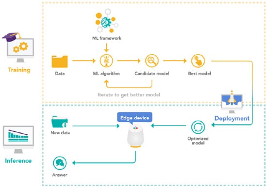
Figure 1.
Overall block diagram of the project [4].
The initial phase, enclosed within the yellow box in Figure 1, is dedicated to the training of Machine Learning Models on a host machine (PC). During this phase, the Integrated Development Environment (IDE) on the host machine is used to develop and deploy an application onto an edge device. This application facilitates the acquisition of vibration data from an FXOS8700CQ—3-axis 14 bit-accelerometer. The acquired vibration data then serve as the input dataset for machine learning algorithms, facilitating the training of multiple models. These models, employing diverse algorithms, are iteratively developed as candidate models and benchmarks until an optimized model is achieved. A thorough evaluation of widely used fault detection algorithms (described in Table 1), such as Support Vector Machines (SVM), K-Nearest Neighbors (K-NN), Random Forest Classifier (RF), Gradient Boosting Classifier (GB) and Convolutional Neural Network (CNN), is conducted to select the best candidate model. The chosen model is subsequently converted to a TensorFlow framework for deployment on the edge device.

Table 1.
Commonly Used Machine Learning Methods.
Upon the completion of the first phase in Figure 1, the project seamlessly progresses to the second phase, denoted by the green box. In this phase, the optimal model derived from the initial training is deployed onto the edge device. This model operates in real time, providing predictions as new data are introduced to the device. The device, in turn, assesses the state of the fan and produces a corresponding output.
2.2. Overview: Machine Learning Methods
Table 1 provides an overview of the most commonly used ML methods for Predictive Maintenance. The first column represents the paper reference; the second column lists the ML method; the third column lists the type of equipment on which maintenance prediction is performed; the fourth column lists the type of data; and the fifth column provides the accuracy of the machine learning model.
For the task of supervised machine learning, a “Classification” model is selected over a “Regression” model because the desired output (label) is discrete. Furthermore, neural network algorithms are preferred due to their high accuracy as compared to other algorithms. However, traditional ML models are also evaluated in this paper to compare the performance of different types of models, including the commonly used traditional ML models, listed in Table 1, to determine the best model for the task at hand, i.e., fault detection in an electric fan drive.
2.3. Advantages of CNNs for Vibration Signal Analysis
Convolutional neural networks (CNNs) are preferred over artificial neural networks (ANNs) due to their ability to reduce the number of network parameters using filters or “kernels”. ANNs become computationally expensive when increasing the number of hidden layers and neurons due to their fully connected nature, whereas CNNs have sparse connections between layers. CNNs also consider both node strength and spatial positions, improving accuracy and reducing overfitting. They are specifically suited for data with spatial structures like images, videos, and sensor data such as accelerometers. Vibration signals exhibit short-term patterns captured by local receptive fields and global patterns captured by deeper CNN layers. Recurrent neural networks (RNNs) [10], designed for temporal data, may not be optimal, as vibration signals lack long-term dependencies.
In addition, CNNs require fewer pre-processing steps and can learn filters automatically, eliminating the need for manual feature engineering in primitive methods. Therefore, given that the input data are derived from accelerometer sensor readings, CNNs are the preferred approach for this project. In the later part of this paper, it is shown that the CNN model is indeed the best choice when compared to other ML models.
2.3.1. Convolutional Neutral Network
- (1)
- Convolutional layer
Typically, CNNs consists of an input layer, output layer, and hidden layers [11]. The following formula can be used to represent the mathematical model of a convolutional layer [11,12]:
The (∗) denotes the dot products of the convolutional operation; Mj denotes the number of input maps; l denotes the network’s lth layer; k denotes the kernel matrix, which has the dimensions S × S (for example, a kernel size of 3 × 3), and f is the non-linear activation function. There is a multiplicative bias and an additive bias b assigned to each output map, but its exact form depends on the specific pooling method used [8,12].
- (2)
- Non-linear activation function
Non-linear activation functions are needed to transform the output of a neuron from a linear combination of inputs to a non-linear function of those inputs. The linear operation output, such as convolution, from the previous layer is passed through these activation functions. Common non-linear activation functions used in neural networks include the Rectified Linear Unit (ReLu), Tanh and Leaky ReLu. The mathematical equations, [13,14] for the activation functions, are given by:
- (3)
- Pooling layer
Pooling layers are used to reduce the dimensionality of the input and extract dominant features which can be defined by:
The sub-sampling function is expressed by down(.). The output is often n times smaller along both spatial dimensions, because this function sums over each distinct n-by-n block in the input [8]. The most common pooling method is max pooling [11], which divides the input image into non-overlapping rectangles and outputs the maximum value for each sub-region.
- (4)
- Fully connected layer
In the final fully connected layer, a SoftMax function [13] is often selected which normalizes the output values from the last fully connected layer to perform multi-class classification [11]. The mathematical definition of the SoftMax function is
The multi-class classifier has K classes in total. values are the input vector’s components and can have any real value. The normalization term, which lies at the denominator of the equation, ensures that the function’s output values will all add up to 1, creating a valid probability distribution.
2.3.2. Design and Development
- (1)
- Data Collection
A new dataset of time series sensor data is required for this work due to variations in sensor type and positioning. For demonstration purposes in this project, a small DC 5V, 0.20A server cooling fan is utilized. However, it should be noted that in real-world applications, industrial size fans would be considered instead of the small test fan we are using here.
A dataset of time-series sensor data is collected using the development board (FDRM-STBC-AGM01) with an FXOS8700CQ accelerometer (3-Axis Sensor). The embedded application reads the vibration data from the accelerometer and logs them onto an SD card. Data collection is conducted for 10 min for each class (Fan-Fault, Fan-On and Fan-Off), resulting in a total of 120,000 samples for each class (recording at 200 Hz). To elaborate on the specific states:
- Fan-On State: no external vibration source was introduced. The data solely represent the vibration patterns collected from a normally operating fan.
- Fan-Off State: the fan was turned off during data collection.
- Fan-Fault State: devices were used to interfere with the fan blades and hence induce vibration and disturb the normal operation of the fan. These devices were placed on different locations of the fan, each with varying levels of vibration. This approach aimed to cover a diverse range of vibration scenarios, ensuring the robustness and generality of the data.
The collected data, encompassing fan states, sample time and accelerometer readings, are saved as CSV files on the SD card, with subsequent transfer to the host machine for ML model training. Figure 2 shows the time-domain plot of the input signal obtained from the data collection stored on the SD card. The x-axis of the plot represents the time sequence, while the y-axis represents the amplitude of each point in that sequence, ranging from −8192 to +8192 units (corresponding to a range of ±2 g). For enhanced visualization, Figure 3 offers a zoomed-in view within the scale of −2000 to +2000.
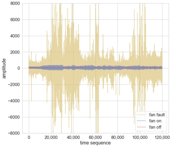
Figure 2.
Time sequence plot of the input signal.
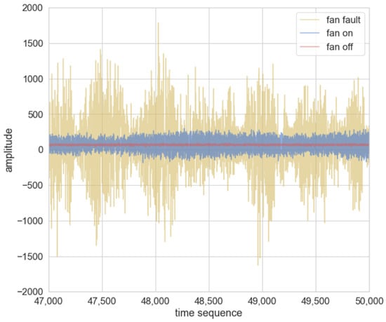
Figure 3.
Zoomed-in view of Figure 2.
The vibration signals of the fan in different states exhibit distinct characteristics:
- Fan-On (Blue): The signal is smooth, continuous waveform with only small amplitude variation over time.
- Fan-Off (Red): The signal is flat with minimal variation, indicating little to no vibration due to the absence of fan rotation.
- Fan-Fault (Yellow): The signal has an irregular waveform with significant amplitude variation, resulting from the higher frequency vibrations caused by friction.
It is important to use the same size of training dataset for each class to avoid any biased predictions on unseen data. Figure 4 shows that the dataset is balanced and distributed equally for each class.
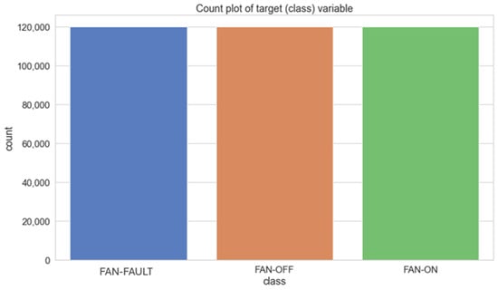
Figure 4.
Imported dataset for training.
- (2)
- Data pre-processing
The data pre-processing step is crucial for reducing processing time and improving the quality of the data. We conducted the following pre-processing procedures, adapted from “The Ten-Step machine learning methodology” [15]:
- Data checking and cleaning: Duplicated or irrelevant data were removed to ensure accurate and reliable analysis.
- Data normalization: Scaling the features to a common range improves the performance of ML models and prevents over-reliance on certain features. The signal is scaled to a new range of [−1, 1] instead of [0, 1], because the sign of the signal can be preserved for vibration signals which contain both positive and negative values. An approach was adopted to normalize the data from 0 to 1; however, this resulted in a model with poorer accuracy. The normalization equation [16] that is used in this project is given by:
- 3.
- Feature Selection: Only the most relevant features (X, Y, Z axes of vibration signals) were selected for the classification task of fan states, reducing dimensionality and improving model performance.
- 4.
- Train–Test Split: Separating the entire data set into a training set and a test set is another pre-processing step. The separation of the data prevents information from the test set from leaking into the training set. This method is typically used to assess the model’s overall performance during training and then cross-validate it against the test set. The true purpose of data splitting is to allow the network to forecast vibration characteristics from previously unseen data (i.e., data not used during training).
In this project, the data were divided at random into 80% and 20% for training and testing. Figure 5 depicts the dataset split into the training and test datasets.
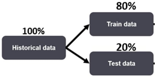
Figure 5.
Train-Test Split.
- 5.
- Data Reshaping: This step is crucial to ensure the model can handle the inputs. The vibration signals are reshaped into 2D tensors instead of 1D tensors to capture correlations and patterns across multiple dimensions. The three axes (X, Y, Z) in the vibration signal represent different correlations and patterns that can be observed in these dimensions. This enables a more comprehensive analysis of the signal, making it easier to identify complex patterns and features that may not be evident in a 1D tensor. In addition, CNNs are well-suited for handling 2D tensors, as they excel in capturing correlations and patterns in image-like data.
- (3)
- Network Architecture
Hyperparameters such as network architecture, learning rate, and activation functions were tuned in the training stage to achieve the best performance on the test dataset [17]. Figure 6 presents the process of model training and parameter tuning. The blue blocks (historical data, train data and test data) are the fixed input whereas the black blocks (hyperparameters, model training and model) are the volatile parameters, and the green blocks (train evaluation matrices and test evaluation matrices) are evaluated outputs. The output of the test data is passed back to the hyperparameter to obtain the most optimal hyperparameters [17,18].
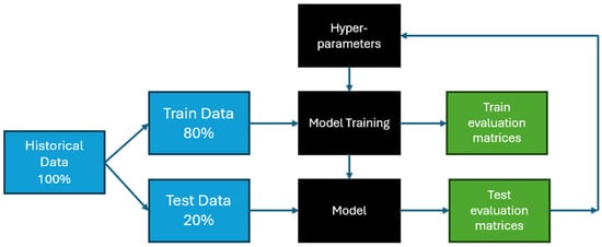
Figure 6.
Model training and parameter tuning.
The process involved manual adjustment of each parameter. To compare different models, nine experimental test groups were considered. The number of convolutional layers and activation functions in each layer were varied individually in the group. The accuracy of each combination was recorded in Table 2.
Table 2.
Results of the nine experimental groups.
From Table 2, Experimental Group 1 and Group 9 achieved the highest accuracy scores (Please refer to Figure A1 in Appendix A for the training history for Experimental Group 1). The model based on Experimental Group 1 was chosen due to its lower computational cost and faster training process. This was because Group 1 had fewer convolutional kernels and overall parameters compared to Group 9.
The CNN architecture used in this study, which was achieved through hyperparameter tuning in Experimental Group 1, is shown in Figure 7. It comprises three convolution layers with filter counts of 8, 16, and 32, each with a 3 × 3 size. These layers are followed by MaxPooling [12] and dropout layers with dropout rates of 50%, 20% and 20%, respectively. The selection of a 3 × 3 kernel is based on the need to classify vibration signals with three axes, allowing the capture of spatial information along all three axes for precise classification. A 3 × 1 or 1 × 3 kernel would only capture information along one or two axes, respectively, which may not be enough for signals that have three axes.
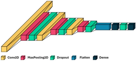
Figure 7.
Modified CNN Architecture.
The use of pooling and dropout layers greatly reduces the number of parameters in the fully linked layers and hence decreases training time.
The architecture is a sequential model in Keras, which is a linear stack of layers. It consists of several types of layers: Conv2D, MaxPooling2D, Dropout, Flatten, and Dense. The model starts with an input layer of shape (batch_size, 128, 1, 3) and the number of parameters for this layer is not shown since it does not have any trainable parameters.
The details of each layer are explained as follows:
- -
- The first layer is a Conv2D layer that executes 2D convolution on the input data. The layer employs the ReLu activation function and has eight filters of size (3 × 3), which means that it will produce eight feature maps, each of size (128, 1). ‘Same’ padding is used to ensure the output size is the same as the input size. The layer’s output shape is (None, 128, 1, 8), where None can be considered as a placeholder for the batch size of the input.
- -
- The second layer is a MaxPooling2D layer that maximizes pooling over the output results of the previous layer. The pool size is (2, 2), has strides of (2, 2) and “same” padding, so the output shape of this layer is (None, 64, 1, 8), which is half the dimensions of the output features.
- -
- In the third layer, a dropout layer with a rate of 0.5 is used which applies dropout regularization to the output of the previous layer, randomly dropping out 50% of the units. This layer has no output shape, as it only affects the training process and has no trainable parameters.
- -
- The fourth layer is another Conv2D layer using 16 filters of a size of 3 × 3 with the ReLu activation function. This layer’s final output form is (None, 64, 1, 16).
- -
- Similarly, in the fifth layer, another MaxPooling2D layer with pool size (2, 2), strides of (2, 2) and “same” padding is applied. The output shape of this layer is reduced by half to (None, 32, 1, 16). This layer is again followed by a dropout layer with a rate of 0.2 to avoid overfitting. A relatively low dropout rate, like 0.2, implies that during training, 20% of the neurons in the layer are randomly “dropped out” at each update. The lower dropout rate in the initial layers allows the network to retain more information in the low-level features, providing a smoother learning curve at the beginning of training.
- -
- The seventh layer is the third convolutional layer, with 32 filters of size (3 × 3) and the ReLu activation function. This layer’s final output form is (None, 32, 1, 32).
- -
- The eighth layer is another MaxPooling2D layer that performs max pooling over the output of the previous layer. The pool size is (2, 2), which means that the output shape of this layer is (None, 16, 1, 32).
- -
- The ninth layer is another dropout layer with a rate of 0.2.
- -
- The tenth layer is a Flatten layer that flattens the output of the previous layer into a 1D vector. The output shape of this layer is (None, 512).
- -
- The eleventh layer is a fully connected layer with 128 units and uses the ReLu activation function. The output shape of this layer is (None, 128).
- -
- The twelfth and final layer is another dropout layer with a rate of 0.5 followed by a Dense layer with three units, which represents the number of classes in the output. This layer uses the SoftMax activation function, which outputs a probability distribution over the classes. The output shape of this layer is (None, 3).
- -
- The model complies with categorical cross-entropy loss function and Adam optimizer [19]—an upgraded version of the stochastic gradient descent to train the network and revise the weights iteratively according to training data, since they are commonly used for multi-class classification problems. An accuracy metric is used to assess the performance of the model because all classes in the dataset are balanced, and each class is equally important.
Once the CNN architecture has been defined, the training process is initialized. From the training data set, the model parameters (such as weights, biases) are automatically configured by the network itself through the training process.
The model has a total of 72,083 parameters, all of which are trainable. This architecture is commonly used for image classification tasks, with the convolutional layers extracting features from the input image and the fully connected layers performing the final classification.
Table 3 provides a detailed summary of the CNN model. The trainable parameters are the weights and biases of the model that are updated during the training. In the proposed model architecture, there are a total of 72,083 trainable parameters, which are defined by Equation (8) for convolution layers and Equation (9) for dense layers, respectively:
where:
added 1 due to the bias term for each filter.
Table 3.
Detailed description of the CNN model architecture used in this research.
There are eight filters in the first convolution layers, each of size 3 × 3, with three channels per filter as input number of filters, giving rise to a total of 224 trainable parameters, calculated as follows:
Summarizing using Equations (8) and (9), we have:
Similarly, the number of parameters is calculated for the remaining convolution layers as:
3. Results
3.1. CNN Model Accuracy and Loss
Figure 8 shows the training and validation accuracy plotted against epoch. The training dataset is used to train the generated CNN model, while the test dataset is used to assess the performance. As the number of epochs increases, accuracy increases and loss decreases. At epoch 25, there is no appreciable gain in accuracy or loss; hence, a total of 30 epochs were used for training and testing. Using the categorical cross-entropy loss function, the test accuracy is 99.82% and the training accuracy is 99.80%, indicating that the model is not overfitting. Moreover, the loss for the training dataset and the test dataset is 0.0048 and 0.0152, respectively. This indicates that the model can generalize effectively to the unseen vibration data.
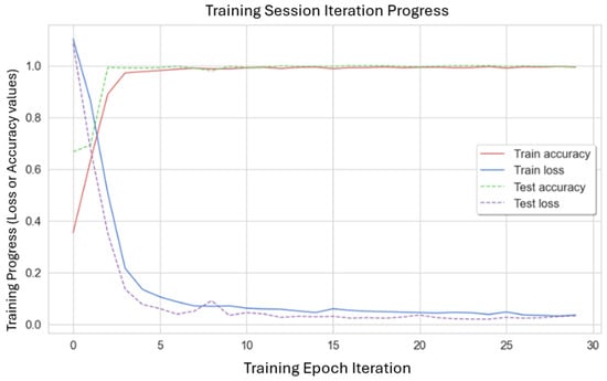
Figure 8.
Training and Validation Accuracy vs. Epoch.
To analyze the performance of the machine learning model or algorithms in more detail, it is essential to use evaluation metrics. The confusion matrix is one metric that measures how accurate a classification model is. It is an N × N matrix that compares the actual example data with those calculated by the ML model, where N is the number of target classes [18].
The classification problem in this project has three classes. Therefore, the confusion matrix used to evaluate the performance of the model has three rows and three columns, with a total of nine values. The confusion matrices for the full dataset, training dataset, and validation dataset are shown in Figure 9, Figure 10 and Figure 11, respectively. The columns represent the actual values of the fan classification, while the rows in the matrix represent the predicted values of the fan class. Note that the input dataset used in this project is balanced, meaning that it contains an equal number of samples for each class of a fan state. Hence, equal percentages are distributed to each class of the fan state.
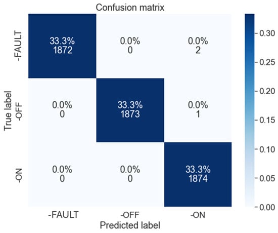
Figure 9.
Confusion matrix for the full dataset.

Figure 10.
Confusion matrix for the train dataset.
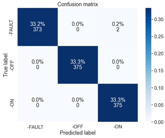
Figure 11.
Confusion matrix for the test dataset.
In addition, the model’s performance can be evaluated using performance evaluation indices such as the accuracy, precision, recall, and F1-score, which are provided by Equations (10)–(13):
where TP = True Positive, TN = True Negative, FP = False Positive, and FN = False Negative [20,21].
Table 4 shows that the model has high accuracy and performs well for all three fan states. The fan-off state has the highest scores, indicating that the model can classify this state with high accuracy. This may be because the features from the Fan-Off state were more informative and distinctive compared to the other two states.
Table 4.
Proposed CNN’s performance metrics of the fault labels.
3.2. ML-Based Models Validation
To verify that the CNN model is best suited for the problem of fault detection in a fan drive, several other ML techniques were evaluated. We considered SVM, K-Nearest Neighbor, Random Forest, and Gradient Boosting. These ML-based models were further evaluated in two distinct groups. The first group was trained using raw input signals, while the second group utilized time-domain and frequency-domain features extracted from these raw signals. This is done to compare the performance of the models trained on the two different types of input data and to identify the most effective strategy.
In the development of the second group of ML-based models, the statistical features in the time domain were used. Python code was developed that can extract time-domain features such as mean, variance, crest, skewness, root mean square, and shape factor.
It was found that the sets of models using the extracted time and frequency domain features outperformed the models solely trained on raw input signals. This could be due to the model receiving more relevant and discriminative information when time-domain characteristics are extracted from the raw input signals.
Figure 12 shows the confusion matrix for the ML-based model trained on raw input signals in the first group. In addition, Figure 13 shows the confusion matrix for the ML-based model trained on statistical features in the second group. These confusion matrices provide a visual representation of the performance of each model, in terms of correctly and incorrectly classified samples for each class.
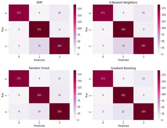
Figure 12.
Confusion matrix for the first group.
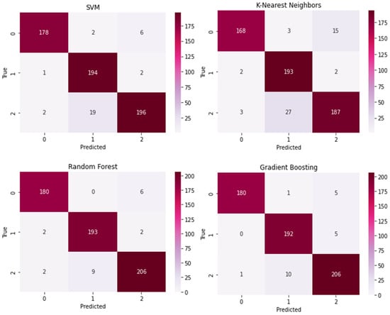
Figure 13.
Confusion matrix for the second group.
The calculated values of accuracy, precision, recall, and F1-score for each class of the fan can be observed in Table 5 for both sets of ML-models. The table compares the obtained performance metrics of different states of the fan using four ML-based models (SVM, RF, K-NN and GB).
Table 5.
Comparison of the performance metrics of different states of the fan.
In addition, the overall performance metrics of the models are summarized in Table 6. Note that the accuracy of the Support Vector Machine (SVM), Random Forest (RF), K-Nearest Neighbors (k-NN), and Gradient Boosting (GB)-based classifiers using raw signals is 91.167%, 91.333%, 90.000%, and 92.500%, respectively. Meanwhile, the accuracy of the models using statistical features is 94.667%, 96.500%, 91.333%, and 96.167%. The traditional ML approach requires feature extraction and selection, which is a difficult operation that calls for prior knowledge and skill.
Table 6.
Comparison of overall performance metrics.
It is observed that the models using statistical features have higher accuracy than the models using raw signal inputs. In addition, bar plots are created to visually compare the performance of each model (please refer to Figure A2 in Appendix A).
3.3. Model Comparison with Traditional ML-Based Models
The results of these ML-based (SVM, RF, K-NN, GB) models are compared against the results of the CNN model, as shown in Figure 14 and Figure 15 for group 1 and group 2, respectively. The bar plots in Figure 15 show that CNN still achieved the highest accuracy, even higher than that of models using statistical features.
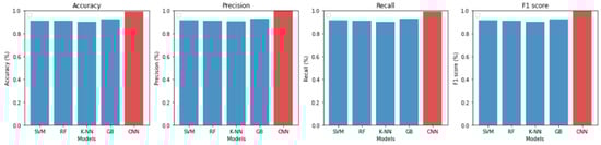
Figure 14.
Performance of CNN model vs. ML-based models (group 1).
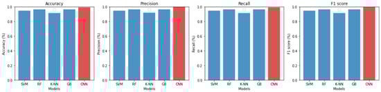
Figure 15.
Performance of CNN model vs. ML-based models (group 2).
In summary, these results suggest that the developed CNN model is the most suitable model for this specific classification task, outperforming the ML-based models using raw input signals and those using statistical features. It achieved the highest accuracy among all ML-based models without requiring any feature extractions. The CNN model proved to be more effective and efficient, as it supports automatic feature extraction, giving it an advantage over traditional machine learning methods. Therefore, this CNN model is selected, exported, and deployed on an embedded device to make real-time predictions.
3.4. Model Deployment on Edge Device
After the optimized model was developed, as described in the previous section, the model was then deployed on the embedded device. To integrate the proposed ML model with a real-time application for end-users, the following steps were meticulously undertaken:
- Model Deployment: The trained ML model was deployed on an embedded machine for real-time predictions. This deployment leveraged the LPCXpresso55S69 embedded microcontroller and the FXOS8700CQ three-axis accelerometer from NXP, ensuring seamless compatibility with the target environment.
- Utilization of NXP’s Repository: NXP’s repository played a pivotal role in this integration. Specifically, it housed the ML-Based System State Monitor App Software Pack, streamlining the deployment process. This software pack, designed for MCU-based systems, aligns seamlessly with the overall system architecture.
- MCUXpresso SDK Integration: The integration was further facilitated by utilizing the MCUXpresso SDK as the Integrated Development Environment (IDE) on the host machine. This SDK ensured the smooth delivery of the overall system.
- Consideration of Variations: It is important to note that for different types of fan applications, the collection of a new data set is essential to train the model. Variation in the positioning of sensors necessitates tailored datasets to ensure optimal model performance.
4. Discussion
The following points can be made when discussing the outcomes on a broader scale:
- Despite the availability of several common convolutional models like Google Net, AlexNet, or Mobile Net, using a simpler model has the benefits of creating a small but highly efficient model that is straightforward to install on low-power edge devices. A simple model guarantees quick calculations, little memory usage, and preserves the device’s capability for real-time classification.
- Although it works with a small dataset which is collected for only 30 min, the CNN can be trained properly with enough training samples.
- This project has been tested on data from a real-world scenario, which would potentially perform well when implemented on a large industrial fan drive. The model can be applied to other types of machinery if they produce vibration signals that can be recorded by an accelerometer and analyzed using the same methodology. For instance, the model can find applications in smart door systems. Anomalies, such as attempted break-ins or hacking attempts, manifest as distinct vibration patterns during unauthorized door access. This triggers anomaly detection, notifying users of potential security breaches. However, the training data would need to be collected and labeled specifically for each type of machinery.
- The use of window slicing allows CNN models to extract more meaningful features from the signal and improve the accuracy of the algorithms, similar to how convolutional layers in CNNs extract features from images. The overlap ratio is also used to ensure that the windows are not completely independent of each other, allowing the model to capture the temporal relationship between adjacent windows.
- Accuracy, precision, recall, and F1-score were used as performance metrics to assess the performance of the developed models. It was found that the CNN model achieved the highest performance results even though it was trained using the raw input signals.
- Although it is well known that deeper networks frequently have more accuracy than shallow networks, they also have a high computational cost. They also have large computational footprints, which can delay the prediction time in a real-time classification problem. This study demonstrates that the CNN architecture developed in this project will yield the ideal model (considering both accuracy and low computational costs) that needs to be deployed on low-power edge devices like microcontrollers.
- It is noteworthy that the current model is trained for specific fan positioning. To extend the applicability of the algorithm to different machinery or alternative fan positions, the acquisition of tailored training data will be necessary.
5. Conclusions
In conclusion, this project sought to establish a robust framework for real-time fault detection in vibration signals through an embedded device. The investigation encompassed a comprehensive review of prevalent machine learning algorithms. Additionally, a streamlined Convolutional Neural Network (CNN) model was meticulously crafted, emerging as the optimal choice due to its innate ability for automatic feature extraction. Key Novelties:
- Embedded Machine Learning Approach: Successfully introduced an embedded machine learning approach, laying the foundation for real-time anomaly detection in the context of fan motor health monitoring.
- Diverse Algorithm Exploration: Conducted an in-depth analysis and development of commonly used ML algorithms, encompassing SVM, K-NN, Random Forest, and Gradient Boosting Classifiers.
- Optimization of CNN Model: Tailored a CNN model specifically for vibration signals, incorporating automatic feature extraction and simplified data pre-processing techniques to enhance fault detection accuracy.
- Cost-Effective Design: Strategically designed to be cost-effective, ensuring accessibility for a broad audience, including individuals and businesses.
- Versality Across Industries: Demonstrated the versatility of the developed model, showcasing its potential applications across various industries, if vibration signals are recordable by an accelerometer.
These key novelties collectively position this study at the forefront of advancing machine learning applications in the realm of industrial fan health monitoring. This project has been tested on data from a real-world scenario, which would potentially perform well when implemented in an industrial setting. The model can be applied to other types of machinery if they produce vibration signals that can be recorded by an accelerometer and analyzed using the same methodology. For instance, the model can find applications in smart door systems. Anomalies, such as attempted break-ins or hacking attempts, manifest as distinct vibration patterns during unauthorized door access. This triggers anomaly detection, notifying users of potential security breaches. However, the training data would need to be collected and labeled specifically for each type of machinery. The successful integration of these innovations not only contributes to the academic understanding of fault detection methodologies but also holds promise for practical, real-world implementations with widespread accessibility.
6. Future Work
The limitation of the current system is the model is that the model is currently trained for a specific fan and its specific positioning of both the fan and the accelerometer. To address this limitation, further research and development are needed to enhance the algorithm’s capability to detect different types of machinery and various positions of the fan and the accelerometer. In addition, exploring the intersection of quantum computing with artificial intelligence, particularly quantum convolutional neural networks [20], could offer novel approaches to machine learning tasks. Our future work includes incorporating quantum algorithms and computing methods which may lead to advancements in the efficiency and computational capabilities of fault detection systems.
Author Contributions
Conceptualization, Data Curation and Investigation, K.H.H.A.; Methodology, Resources and Software, Supervision, Funding Acquisition, C.L.K.; Project administration, Visualization, Supervision and Formal analysis, Y.Y.K.; Supervision and Funding Acquisition, T.H.T. All authors have read and agreed to the published version of the manuscript.
Funding
This research received no external funding.
Data Availability Statement
The data presented in this study are available on request from the corresponding author. Unavailable due to privacy.
Acknowledgments
The authors would like to extend their appreciation to the University of Newcastle, Australia, for financing the project possible.
Conflicts of Interest
The authors declare no conflict of interest.
Appendix A
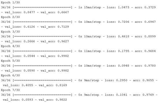
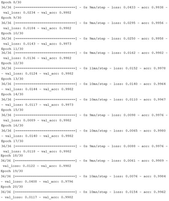
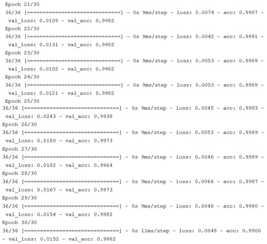
Figure A1.
Training history for Experimental Group 1.
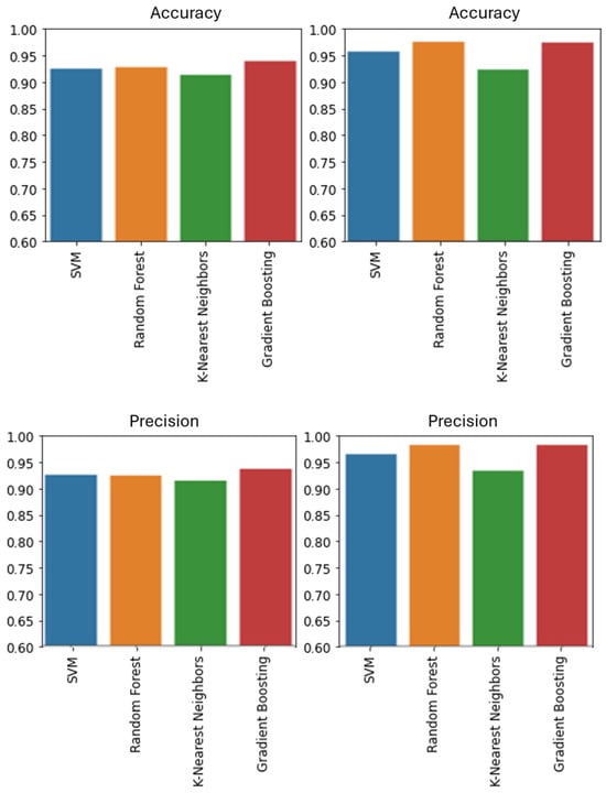
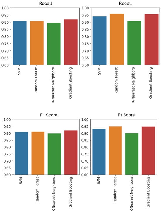
Figure A2.
Comparison of the performance matrix between models using raw signals (left) and models using statistical features (right).
References
- Kay, S.; Kosmas, D.; Jens, W. Machine Learning Techniques for structural health monitoring. In Proceedings of the 8th European Workshop on Structural Health Monitoring (EWSHM), Bilbao, Spain, 5–8 July 2016; p. 1. Available online: https://www.researchgate.net/publication/303933051_Machine_learning_techniques_for_structural_health_monitoring (accessed on 21 October 2022).
- Suda, N.; Loh, D. Machine Learning on Arm Cortex-M Microcontrollers. White Paper, 2019. Available online: https://www.arm.com/resources/guide/machine-learning-on-cortex-m (accessed on 12 March 2023).
- Tensor Flow. Tensor Flow Lite for Microcontroller. Tensor Flow, 2022. Available online: https://www.tensorflow.org/lite/microcontrollers (accessed on 11 November 2022).
- NXP Semiconductors. Image from NXP Catalogue. In NXP Catalogue; NXP Semiconductors: Eindhoven, The Netherlands, 2018. [Google Scholar]
- Praveenkumar, T.; Saimurugan, M.; Krishnakuma, P.; Ramachandran, K.I. Fault Diagnosis of Automobile Gearbox Based on Machine Learning Techniques. Procedia Eng. 2014, 97, 2092–2098. Available online: https://www.sciencedirect.com/science/article/pii/S187770581403522X (accessed on 15 November 2022). [CrossRef]
- Su, C.J.; Huang, S.F. Real-time big data analytics for hard disk drive predictive maintenance. Comput. Electr. Eng. 2018, 71, 93–101. [Google Scholar] [CrossRef]
- Vives, J. Monitoring and Detection of Wind Turbine Vibration with KNN-Algorithm. J. Comput. Commun. 2022, 10, 1–12. [Google Scholar] [CrossRef]
- Hoang, D.-T.; Kang, H.-J. Rolling element bearing fault diagnosis using convolutional neural network and vibration image. Cogn. Syst. Res. 2019, 53, 43–50. [Google Scholar] [CrossRef]
- Qin, J.T.C.; Li, W.; Liu, C. Intelligent Fault Diagnosis of Diesel Engines via Extreme Gradient Boosting and High-Accuracy Time-Frequency Information of Vibration Signals. Sensors 2019, 19, 3280. [Google Scholar] [CrossRef]
- Saeed, M. An Introduction to Recurrent Neural Networks and the Math That Powers Them. September 2022. Available online: https://machinelearningmastery.com/an-introduction-to-recurrent-neural-networks-and-the-math-that-powers-them/#:~:text=A%20recurrent%20neural%20network%20 (accessed on 11 November 2022).
- Yamashita, R.; Nishio, M.; Do, R.K.G.; Togashi, K. Convolutional neural networks: An overview and application in radiology. Insights Imaging 2018, 9, 611–629. [Google Scholar] [CrossRef] [PubMed]
- Yani, M.; Irawan, S.; Setianingsih, C. Application of Transfer Learning Using Convolutional Neural Network Method by Early Detection of Terry’s Nail. J. Phys. Conf. Ser. 2019, 1201, 12052. [Google Scholar] [CrossRef]
- Miranda, L.J. Understanding Softmax and the Negative Log-Likelihood. ljvmiranda921.github.io, 2017. Available online: https://ljvmiranda921.github.io/notebook/2017/08/13/softmax-and-the-negative-log-likelihood/ (accessed on 10 March 2023).
- Paoletti, M.E.; Huat, J.M.; Plaza, J.; Plaza, A. Deep Learning Classifiers for Hyperspectral Imaging: A Review; Hyperspectral Computing Laboratory (HyperComp), Department of Computer Technology and Communications, Escuela Politecnica de Caceres, University of Extremadura, Avenida de la Universidad s/n: Caceres, Spain, 2019. [Google Scholar]
- Giannelos, S.; Moreira, A.; Papadaskalopoulos, D.; Borozan, S.; Pudjianto, D.; Konstantelos, I.; Sun, M.; Strbac, G. A Machine Learning Approach for Generating and Evaluating Forecasts on the Environmental Impact of the Buildings Sector. Energies 2023, 16, 2915. [Google Scholar] [CrossRef]
- Ashish, K.S. Normalization Formulat. WallStreetMojo, 2023. Available online: https://www.wallstreetmojo.com/normalization-formula/ (accessed on 2 February 2023).
- F2005636. Evaluating Machine Learning Models Using Hyperparameter Tuning. Available online: https://www.analyticsvidhya.com/blog/2021/04/evaluating-machine-learning-models-hyperparameter-tuning/ (accessed on 12 April 2021).
- Bhandari, A. Everything you should know about Confusion Matrix for Machine Learning. Anal. Vidya 2022, 3, 10. [Google Scholar]
- Kingma, D.P.; Ba, J. Adam: A Method for Stochastic Optimization. arXiv 2014. Available online: https://arxiv.org/pdf/1412.6980.pdf (accessed on 11 November 2022).
- Herrmann, J.; Llima, S.M.; Remm, A.; Zapletal, P.; McMahon, N.A.; Scarato, C.; Swiadek, F.; Andersen, C.K.; Hellings, C.; Krinner, S.; et al. Realizing quantum convolutional neural networks on a superconducting quantum processor to recognize quantum phases. Nat. Commun. 2022, 13, 4144. [Google Scholar] [CrossRef] [PubMed]
- Sokolova, M.; Lapalme, G. A systematic analysis of performance measures for classification tasks. Inf. Process. Manag. 2009, 45, 427–437. [Google Scholar] [CrossRef]
Disclaimer/Publisher’s Note: The statements, opinions and data contained in all publications are solely those of the individual author(s) and contributor(s) and not of MDPI and/or the editor(s). MDPI and/or the editor(s) disclaim responsibility for any injury to people or property resulting from any ideas, methods, instructions or products referred to in the content. |
© 2024 by the authors. Licensee MDPI, Basel, Switzerland. This article is an open access article distributed under the terms and conditions of the Creative Commons Attribution (CC BY) license (https://creativecommons.org/licenses/by/4.0/).