4.1. Classification Metrics for LOCT Dataset
In this section, results averaged across classes are presented for each of the tested models. Values in
Table 3,
Table 4,
Table 5,
Table 6 and
Table 7 contain performance metrics obtained on the test set after applying described preprocessing techniques. The best-observed results for each optimizer are reported in bold.
With the VGG16 model (
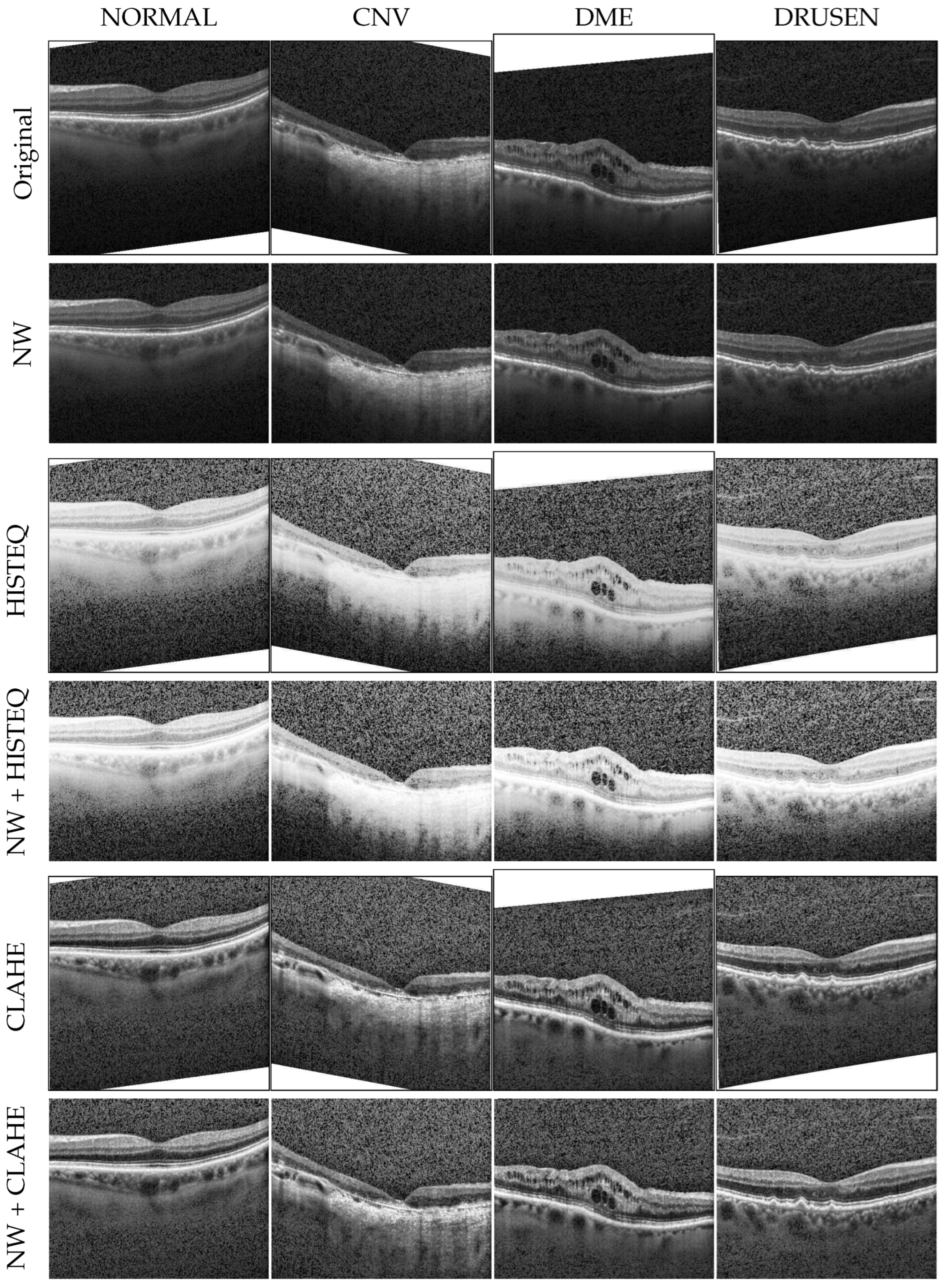
Table 3), performing the CLAHE operation has a clear beneficial impact, whereas applying standard histogram equalization frequently leads to lower accuracy values than expected. The best results of 96.38% for both accuracy and F1-score were achieved with the RMS optimizer after removing white spaces and performing CLAHE operation, although the Adam optimizer gave very similar values.
The InceptionV3 model (
Table 4) gave similarly good results when using the Adam optimizer on
NW data after standard histogram equalization (96.38% accuracy and 96.39% F1-score). Other optimizers performed slightly worse, with best values of 95.97% accuracy for RMS and the
NW dataset and 95.97% accuracy for SGD with HISTEQ. It should be noted that the CLAHE technique was not beneficial when using this model.
The least-observable influence was found in the case of the Xception model (
Table 5). With Adam optimizer, no increase in the accuracy or recall was observed with respect to unprocessed data. The standard histogram equalization gave here a small increase in precision (by 0.07%) and F1-score (by 0.02%). Nevertheless, the best results were obtained when using SGD optimizer with CLAHE on
NW data: 96.49% for both accuracy and recall, and 96.50% and 96.48% for precision and F1-score, respectively. Similarly, a combination of
NW data and CLAHE resulted in improving classification performance for the RMS optimizer.
The greatest influence of preprocessing was observed for the ResNet50 model (
Table 6). Here, with the Adam optimizer, white space removal increased the accuracy of disease classification by 4.13%, resulting in 89.05% as the best value. With RMS and SGD optimizers, an application of CLAHE on
NW allowed for obtaining the best F1-score values of 87.42% and 84.56%, respectively. Notably, all of the best results obtained with the ResNet50 model are lower than for other NN models, from 7.44% (with Adam optimizer) to 11.99% (with SGD).
For the three analyzed optimizers with the DenseNet121 model (
Table 7), the results obtained on the
NW data gave the best F1-scores of 96.17%, 96.59%, and 96.39% for Adam, RMS, and SGD, respectively. However, no clear pattern of impact for the histogram equalization approach can be discerned, as the best accuracy was achieved after CLAHE for Adam optimizer (96.17%), with no equalization for RMS (96.59%), and after applying a standard method for SGD (96.38%).
4.2. Analysis of Influence of Histogram Equalization
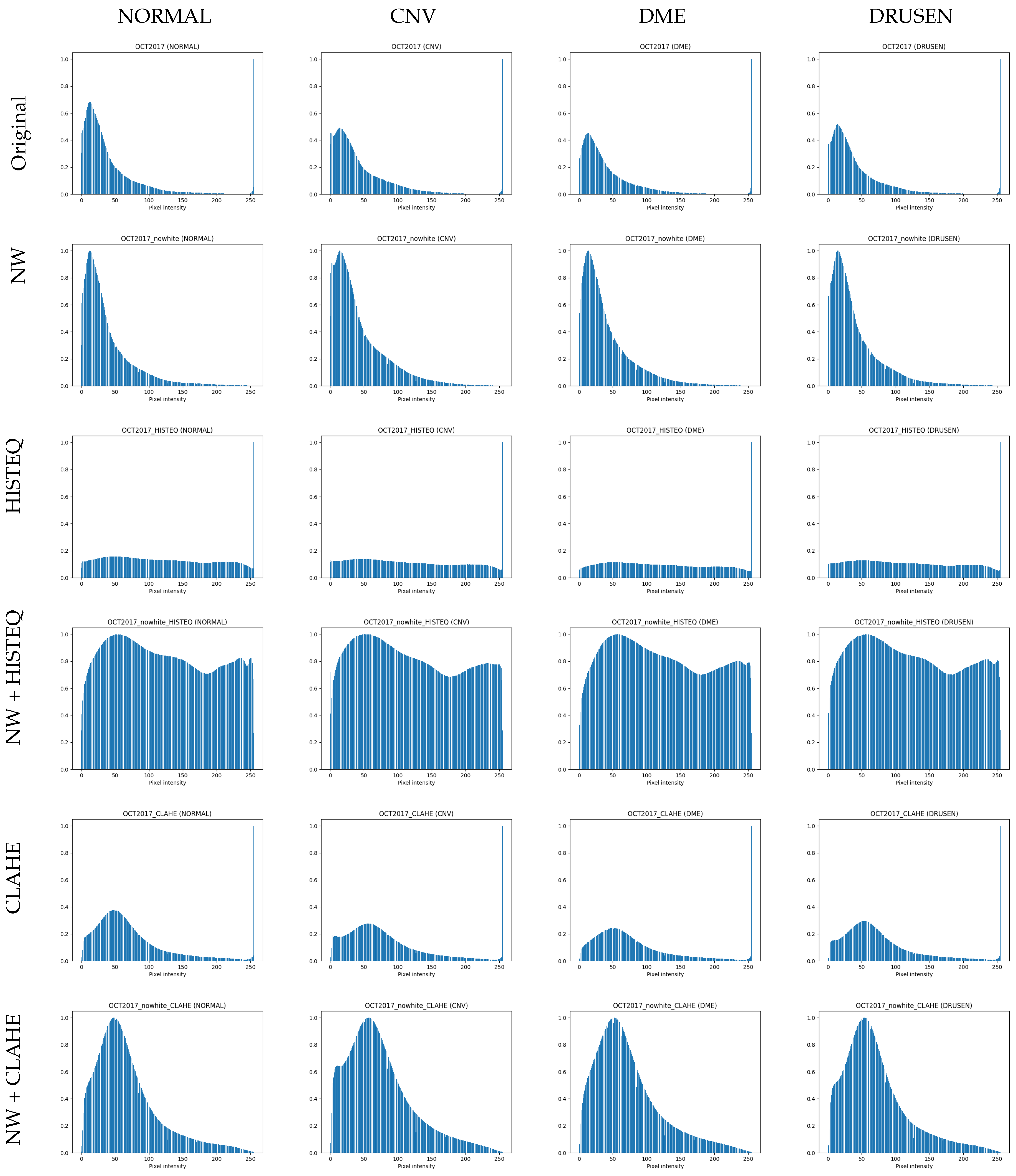
To understand the influence of histogram equalization on OCT images, differences between F1-scores (as a balanced metric) obtained on the original data and images modified with HISTEQ were computed.
Figure 3 presents a bar plot with the calculated values.
What can be observed here is a clear negative impact on classification performance for the ResNet50 model. For all optimizers, the F1-score decreased, with the difference ranging from −4.55% for SGD to −16.26% for Adam. A reduction in F1-score is also noticed in all cases of VGG16, where the metric values dropped by 0.92%, 1.72%, and 2.57% for SGD, RMS, and Adam, respectively. The positive values were obtained for the InceptionV3 model with Adam (0.33%) and SGD (1.24%) and for the DenseNet121 model with RMS (0.3%) and SGD (0.6%).
From an average difference of −2.44% and −0.44% with and without taking into account the ResNet50 results, respectively, it can be summarized that applying simply standard histogram equalization on OCT images decreases the accuracy of disease classification.
A similar analysis conducted for the utilization of CLAHE on original images is presented in
Figure 4. Although the adaptive method enhanced the contrast locally instead of globally (as with the standard histogram equalization), emphasizing characteristics of retina tissue changes, it allowed improving classification only in some cases.
The most dominant change in F1-score was again observed for the ReNet50 model. The CLAHE algorithm seems to positively influence the disease classification process here, as the obtained differences were 3.69% and 8.97% for RMS and SGD, respectively. Overall, with Adam optimizer, the CLAHE does not provide significant gain in the F1-score with an average difference of −0.42% across all models.
Interestingly, a positive difference value was observed in all cases using the VGG16 model (0.09%, 0.93%, and 1.07% for Adam, RMS, and SGD, respectively). Whereas, the Xception model with this method showed a negative change in F1-score across all optimizers (with the difference of −1.11%, −0.52%, and −0.31%, respectively). In conclusion, a beneficial effect can be achieved by applying CLAHE when using the SGD optimizer (with the exception of the Xception model).
4.3. Analysis of Influence of Removing White Spaces
The second analysis was conducted for the impact of removing white spaces from the images.
Figure 5 shows differences in F1-score that illustrate the influence of applying only white space removal (left part of
Figure 5) and combination with standard (central) and adaptive (right) histogram equalization.
For most of the models (regardless of the optimizer used), simple removal of undefined white space at the edge of an OCT image helps in retinal disease classification (left group of the bars in
Figure 5). Negative values here are for VGG16 with Adam (−0.11%) and all Xception models (−0.73%, −0.21%, and −0.1% for Adam, RMS, and SGD, respectively). The positive values range from 0.31% for InceptionV3 with RMS up to 4.04% for ResNet50 with Adam. This preprocessing procedure resulted in a gain of 1.1% on average.
A combination of white space removal and HISTEQ did not lead to significant improvements, as visualized in the central part of
Figure 5. The single most detrimental effect was observed in the case of the ResNet50 model with the SGD optimizer, where the F1-score decreased by 13.92%. The average change for all other models was −0.04%, which is much less than without performing the histogram equalization procedure (as described above). A positive difference value was achieved with InceptionV3 + Adam (0.91%), DenseNet121 + Adam (0.21%), InceptionV3 + RMS (0.5%), Xception + RMS (0.62%), VGG16 + SGD (1.28%), and DenseNet121 + SGD (0.83%). Notably, the gain obtained by removing white spaces was significantly reduced by HISTEQ.
Application of CLAHE on the NW data gave similar results compared to the adjusted dataset with no contrast enhancement. Conversely, negative change values were obtained for the InceptionV3 model (and not Xception as before), with −0.83%, −0.61%, and −0.92% for Adam, RMS, and SGD optimizers, respectively, as well as for VGG16 + SGD (−0.72%) and DenseNet121 + SGD (−0.71%). The overall average change was 0.58%, indicating an improvement in performance, with positive values ranging from 0.21% for VGG16 + RMS to 4.75% for ResNet50 + Adam.
In summary, with Adam and RMS optimizers, it is better to perform white space removal alone or with an application of CLAHE than to apply only HISTEQ or only CLAHE. With SGD optimizer, better results were obtained either on NW data or after performing CLAHE operation, but not when using both. The variations in the F1-score of <1% indicate that the utilized model architectures are robust to small differences in the input data. Another explanation might be that the model has reached a saturation point in performance for the tested dataset, and further procedures might not have a large impact. Overall, the pattern visible in the results suggests that the discussed preprocessing methods depend on the context in which the data are used and the data quality.
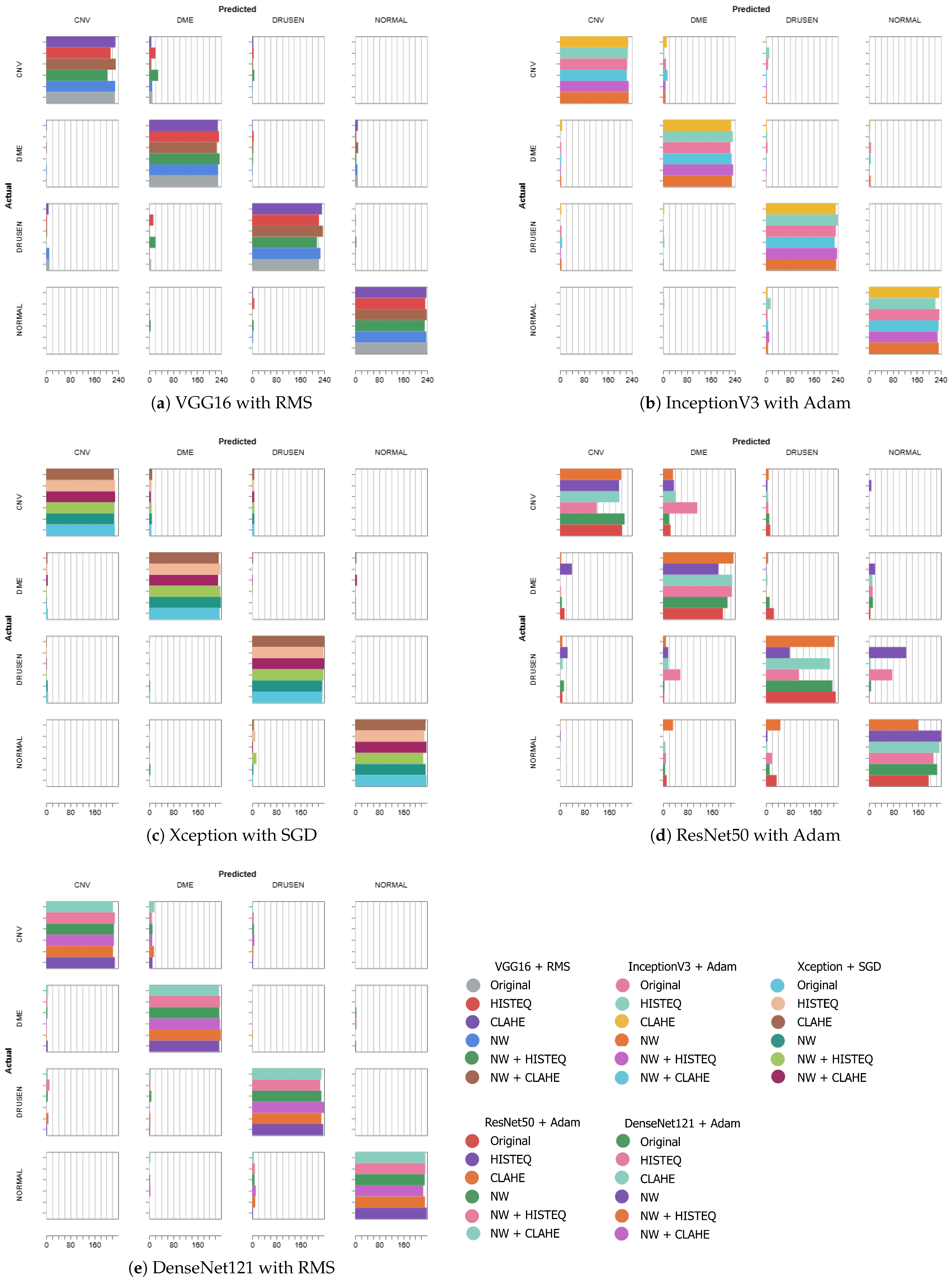
Figure 6 presents the confusion matrices of the best-performing models from each architecture, which are VGG16 + RMS (F1-score of 96.38%), InceptionV3 + Adam (96.39% in F1-score), Xception + SGD (F1: 96.48%), ResNet50 + Adam (F1: 89.06%), and DenseNet121 + RMS (F1: 96.59%). The experiments using the original and NW datasets with described modifications are stacked in the form of horizontal bars to allow for easier comparison between the preprocessing schemes. The diagonal represents the correct predictions, i.e., where the actual label is equal to the predicted label. For each category, in each square, a horizontal bar shows the number of images of the actual label that the model assigned a predicted label. The color indicates the preprocessing method.
Except for the ResNet50 architecture, the best-obtained F1-scores are similar in value. As can be seen in
Figure 6, a majority of the predicted classes can be found on the diagonal (less so for the ResNet50 model—
Figure 6d), which indicates a generally good agreement.
With the VGG16 (
Figure 6a), there occurred more instances of misclassification of CNV (predicted as DME) and DRUSEN (assigned to DME) when utilizing HISTEQ (red) and
NW with HISTEQ (green).
When analyzing plots of the InceptionV3 (
Figure 6b) and Xception (
Figure 6c) models, a similar distribution of the predictions across the preprocessing methods can be observed. Only a few examples of CNV (assigned to either DME or DRUSEN) and NORMAL samples (improperly classified as DRUSEN) are visible, mostly for HISTEQ or
NW + HISTEQ results.
Figure 6d confirms the numerical results obtained for the ResNet model and presented earlier in
Table 6. Here, the majority of misclassification occurred for NW + HISTEQ (pink) and HISTEQ (purple) data, incorrectly assigning CNV (to DME), DME (to CNV), and DRUSEN (to DME and NORMAL). Nevertheless, poor performance was also observed for the CLAHE algorithm (orange) with NORMAL samples (predicted as DME or DRUSEN). Interestingly, all models showed lowered accuracy in distinguishing between CNV and DME samples.
The DenseNet121 model (
Figure 6e) presents a good classification performance, with a low number of inaccuracies (mostly for CNV predicted as DME and NORMAL predicted as DRUSEN). A handful of misclassification instances can be seen for DRUSEN (assigned to CNV) and CNV (assigned to DRUSEN). No significant difference between the preprocessing methods is noticeable in this confusion matrix.


