A Fast Modeling Method for BOR–FDTD

Abstract

Aiming at the inefficiency caused by the optimal design of rotationally symmetric horn feed models, a fast modeling method for rotationally symmetric structures is proposed, which is used to deal with the mesh generation of rotationally symmetric structures and the rapid establishment of computational models. In this paper, the body-of-revolution finite-difference time-domain (BOR–FDTD) method is employed to investigate the radiation performance of the horn feed. Due to the rotational symmetry of the horn antenna, modeling only requires the establishment of a two-dimensional cross-sectional mesh of the horn feed. An optimized Delaunay triangulation algorithm combined with the projection intersection method is utilized to triangulate the horn cross-section of arbitrary polygons and establish the BOR–FDTD computational mesh. Results from both single-medium and multi-medium triangulation algorithms and computational models verify the accuracy of this modeling method. The radiation patterns of a smooth-walled horn were calculated and compared with the modeling time of MATLAB 2017 and the simulation time of CST. The results reveal that the algorithm presented in this paper aligns well with the simulation results from CST; furthermore, the modeling time amounts to only 6.78% of the MATLAB program’s modeling time, while the total simulation time is 31.3% of CST, which demonstrates both the accuracy and efficiency of the proposed method.

1. Introduction

With the rapid development of technology in the field of communication, a well-designed antenna system is more and more important in practical research [1,2]. The horn antenna, as the feed source of the antenna system, is the primary radiator in the whole antenna system, and the model design of the horn antenna will directly affect the performance of the whole antenna system [3,4]. Therefore, the optimized design of the horn antenna is of great significance in studying the performance of the antenna system and how to design an antenna feed with a better performance.

The early design of horn antennas primarily relied on establishing initial models based on analytical models, followed by adjustments to the horn model parameters according to simulation results [5]. This method is time-consuming, labor-intensive, and heavily dependent on the designer’s skill and experience. As antenna systems evolve towards broadband and multiband applications, the design of horn antennas has become increasingly complex and challenging; therefore, traditional design methods have often failed to yield satisfactory results.

The mode-matching method has been widely applied in the design and analysis of narrow-flare-angle horns due to its fast computation speed and high analytical accuracy [6,7]. This method mainly involves cascading typical components as basic structural units to obtain the scattering matrix of the entire horn, which is then combined with plane wave angular spectrum methods or spherical wave expansion methods to derive the radiation pattern of the horn.

Due to the strong electromagnetic coupling effect between the spatial field and the internal field of the large-flare-angle horn, applying the mode-matching method can result in significant errors. Therefore, full-wave analysis methods are more suitable for analyzing the large-flare-angle horn. Common full-wave analysis algorithms include the finite element method (FEM), finite-difference time-domain method (FDTD), and method of moments (MoM) [8,9,10]. Although these methods offer a high accuracy, they require a substantial computational time and memory, leading to a lower optimization design efficiency and even potential task failures.

To address these issues, when analyzing target objects with rotationally symmetric structures, we can extend the traditional FDTD method to the BOR–FDTD method, which makes full use of the rotational symmetry of the model to transform the three-dimensional problem into a two-dimensional electromagnetic problem on a rotationally symmetric plane by applying Fourier series expansion to the electric field and magnetic field components [11,12,13]. Compared with the mode-matching method, the BOR–FDTD method thoroughly considers the interaction between the internal and spatial fields of the horn, exhibiting flexibility in modeling, a wide adaptability, and a high accuracy. Additionally, in contrast to FEM and FDTD methods, the BOR–FDTD method offers faster solution speeds, lower memory usage, and ease of implementation. As the demand for antenna feed systems increases, the application scenarios become more complex, and design specifications become stricter, leading to increased numbers of models, meshes, and optimization iterations. This results in a substantial time consumption and low efficiency in modeling. However, there has been limited research on the fast generation of BOR–FDTD computational models to tackle this issue.

To enhance the efficiency of model optimization and address the demand for rapid modeling of rotationally symmetric structures, an efficient modeling method is proposed. Firstly, the basic theory and recursive formula of the BOR–FDTD method are introduced. Secondly, the Delaunay triangulation algorithm is optimized to accurately transform arbitrary geometric models into triangular meshes. Using the projection intersection method on the triangular meshes of the target surface, the computational model required for BOR–FDTD calculations is obtained. Subsequently, the accuracy of this modeling approach for both single-medium and multi-medium scenarios is validated. Finally, the accuracy and efficiency of this paper’s method are demonstrated by comparing the modeling efficiency of the smooth-walled horn and the results of the radiation patterns.

2. Basic Theory of BOR–FDTD

The BOR–FDTD method expands the components of the electromagnetic field into a Fourier series in the cylindrical coordinate system. After considering the polarization of the incident field, these expansions are substituted into Maxwell’s curl equations for solution. The spatial and temporal differentiation of each field component is replaced with central difference approximations, leading to the derivation of fundamental difference equations used to compute the Fourier coefficients of the field components. For the electromagnetic problems of axisymmetric horn antennas, the BOR–FDTD method significantly reduces computation time and memory consumption, thereby enhancing the computational speed.

In the cylindrical coordinate system, Maxwell’s equations can be expressed as [11]

$$\begin{array}{l}-\mu {\displaystyle \frac{\partial H_{\rho }}{\partial t}}={\displaystyle \frac{1}{\rho }}{\displaystyle \frac{\partial E_z}{\partial \phi }}-{\displaystyle \frac{\partial E_{\phi }}{\partial z}}\\ -\mu {\displaystyle \frac{\partial H_{\phi }}{\partial t}}={\displaystyle \frac{\partial E_{\rho }}{\partial z}}-{\displaystyle \frac{\partial E_z}{\partial \rho }}\\ -\mu {\displaystyle \frac{\partial H_z}{\partial t}}={\displaystyle \frac{1}{\rho }}{\displaystyle \frac{\partial (\rho E_{\phi })}{\partial \rho }}-{\displaystyle \frac{1}{\rho }}{\displaystyle \frac{\partial E_z}{\partial \phi }}\\ \epsilon {\displaystyle \frac{\partial E_{\rho }}{\partial t}}+\sigma E_{\rho }={\displaystyle \frac{1}{\rho }}{\displaystyle \frac{\partial H_z}{\partial \phi }}-{\displaystyle \frac{\partial H_{\phi }}{\partial z}}\\ \epsilon {\displaystyle \frac{\partial E_{\phi }}{\partial t}}+\sigma E_{\phi }={\displaystyle \frac{\partial H_{\rho }}{\partial z}}-{\displaystyle \frac{\partial H_z}{\partial \rho }}\\ \epsilon {\displaystyle \frac{\partial E_z}{\partial t}}+\sigma E_z={\displaystyle \frac{1}{\rho }}{\displaystyle \frac{\partial (\rho H_{\phi })}{\partial \rho }}-{\displaystyle \frac{1}{\rho }}{\displaystyle \frac{\partial H_{\rho }}{\partial \phi }}\end{array}$$

(1)

where $E_{\rho }$, $E_{\phi }$, $E_z$, $H_{\rho }$, $H_{\phi }$, and $H_z$ represent the electric and magnetic field components, respectively, and each component is a function of $\rho$, $\phi$, z, and t. $\rho$, $\phi$, and z are the radial, azimuthal, and altitudinal components in the column coordinate, respectively. $\mu$, $\epsilon$, and $\sigma$ are the magnetic permeability, electrical permittivity, and electrical conductivity, respectively. In the column coordinate, each component of the electromagnetic field is a function of $\phi$ with a period of $2\pi$. Therefore, each field component can be Fourier-expanded with respect to $\phi$ as follows:

$$\begin{array}{l}\mathit{E}(\rho ,\phi ,z,t)={\displaystyle \sum _{m=0}^{\infty }({\tilde{\mathit{E}}}_u(\rho ,z,t)\cos m\phi +{\tilde{\mathit{E}}}_v(\rho ,z,t)\sin m\phi )}\\ \mathit{H}(\rho ,\phi ,z,t)={\displaystyle \sum _{m=0}^{\infty }({\tilde{\mathit{H}}}_u(\rho ,z,t)\cos m\phi +{\tilde{\mathit{H}}}_v(\rho ,z,t)\sin m\phi )}\end{array}$$

(2)

where $\tilde{\mathit{E}}$ and $\tilde{\mathit{H}}$ are the coefficients of the Fourier expansion series, the subscripts u and v denote the cosine and sine functions, respectively, as well as the even and odd functions, and m is the number of modes.

For the rotating body problem, the polarization direction can be defined in the $\rho -z$ plane. The incident field components $E_{\rho }$, $E_z$, and $H_{\phi }$ are even functions and $H_{\rho }$, $H_z$, and $E_{\phi }$ are odd functions. Each field component of the total and scattered fields will maintain the parity of each field component of the incident field, so the components can be expressed as

$$\begin{array}{l}{E}_{\rho }={\displaystyle \sum _{m=0}^{\infty }{\tilde{E}}_{\rho }\cos \left(m\phi \right)}\\ E_{\phi }={\displaystyle \sum _{m=0}^{\infty }{\tilde{E}}_{\phi }\sin \left(m\phi \right)}\\ E_z={\displaystyle \sum _{m=0}^{\infty }{\tilde{E}}_z\cos \left(m\phi \right)}\\ H_{\rho }={\displaystyle \sum _{m=0}^{\infty }{\tilde{H}}_{\rho }\sin \left(m\phi \right)}\\ H_{\phi }={\displaystyle \sum _{m=0}^{\infty }{\tilde{H}}_{\phi }\cos \left(m\phi \right)}\\ H_z={\displaystyle \sum _{m=0}^{\infty }{\tilde{H}}_z\sin \left(m\phi \right)}.\end{array}$$

(3)

Substituting Equation (2) into Equation (1), we can obtain

$$\begin{array}{l}\left[\begin{array}{ccc}0\hfill & -{\partial }_z& -{\displaystyle \frac{m}{\rho }}\\ {\partial }_z\hfill & 0& -{\partial }_{\rho }\\ {\displaystyle \frac{m}{\rho }}\hfill & {\displaystyle \frac{1}{\rho }}(\partial {\rho }_{\rho })& 0\end{array}\right]\left[\begin{array}{l}{\tilde{E}}_{\rho }\\ {\tilde{E}}_{\phi }\\ {\tilde{E}}_z\end{array}\right]=-\left[\begin{array}{l}({\mu }_0{\mu }_{\rho }{\partial }_t+{\sigma }_{\rho }^m){\tilde{H}}_{\rho }\\ ({\mu }_0{\mu }_{\phi }{\partial }_t+{\sigma }_{\phi }^m){\tilde{H}}_{\phi }\\ ({\mu }_0{\mu }_z{\partial }_t+{\sigma }_z^m){\tilde{H}}_z\end{array}\right]\\ \left[\begin{array}{ccc}0\hfill & -{\partial }_z& {\displaystyle \frac{m}{\rho }}\\ {\partial }_z\hfill & 0& -{\partial }_{\rho }\\ -{\displaystyle \frac{m}{\rho }}\hfill & {\displaystyle \frac{1}{\rho }}(\partial {\rho }_{\rho })& 0\end{array}\right]\left[\begin{array}{l}{\tilde{H}}_{\rho }\\ {\tilde{H}}_{\phi }\\ {\tilde{H}}_z\end{array}\right]=-\left[\begin{array}{l}({\epsilon }_0{\epsilon }_{\rho }{\partial }_t+{\sigma }_{\rho }^e){\tilde{E}}_{\rho }\\ ({\epsilon }_0{\epsilon }_{\phi }{\partial }_t+{\sigma }_{\phi }^e){\tilde{E}}_{\phi }\\ ({\epsilon }_0{\epsilon }_z{\partial }_t+{\sigma }_z^e){\tilde{E}}_z\end{array}\right].\end{array}$$

(4)

Equation (4) can be solved for the coefficients of the mth-order term of the Fourier series expansion. By substituting these coefficients into Equation (2) and summing the series, the various field components can be obtained. In practical calculations, Equation (2) is generally taken as $m=1$.

It can be seen that the component $\phi$ is no longer included in Equation (4), thus reducing the computational region from a three-dimensional space to a two-dimensional plane. Then, by replacing the differential form in Equation (4) with the central difference, it is possible to obtain the differential formulation of the BOR–FDTD method, and the iterative formula for the electric field is given by

$$E_{\rho ,m}^{n+1}(i,j)={\displaystyle \frac{2\epsilon -\Delta t\sigma }{2\epsilon +\Delta t\sigma }}{E}_{\rho ,m}^n(i,j)+{\displaystyle \frac{2m\Delta t}{\rho (i+1/2)(2\epsilon +\Delta t\sigma )}}{H}_{z,m}^{n+1/2}(i,j)\hspace{1em}-{\displaystyle \frac{2\Delta t}{\Delta z(2\epsilon +\Delta t\sigma )}}[H_{\phi ,m}^{n+1/2}(i,j)-H_{\phi ,m}^{n+1/2}(i,j-1)]$$

(5)

$$E_{\phi ,m}^{n+1}(i,j)={\displaystyle \frac{2\epsilon -\Delta t\sigma }{2\epsilon +\Delta t\sigma }}{E}_{\phi ,m}^n(i,j)+{\displaystyle \frac{2\Delta t}{\Delta z(2\epsilon +\Delta t\sigma )}}[H_{\rho ,m}^{n+1/2}(i,j)-H_{\rho ,m}^{n+1/2}(i,j-1)]-{\displaystyle \frac{2\Delta t}{\Delta z(2\epsilon +\Delta t\sigma )}}[H_{z,m}^{n+1/2}(i,j)-H_{z,m}^{n+1/2}(i-1,j)]$$

(6)

$$E_{z,m}^{n+1}(i,j)={\displaystyle \frac{2\epsilon -\Delta t\sigma }{2\epsilon +\Delta t\sigma }}{E}_{z,m}^n(i,j)-{\displaystyle \frac{2m\Delta t}{\rho (i)(2\epsilon +\Delta t\sigma )}}{H}_{\rho ,m}^{n+1/2}(i,j)+{\displaystyle \frac{2\Delta t}{\Delta \rho (2\epsilon +\Delta t\sigma )\rho (i)}}[\rho (i+1/2)H_{\phi ,m}^{n+1/2}(i,j)-\rho (i)H_{\phi ,m}^{n+1/2}(i-1,j)]$$

(7)

where $\Delta t$ is the time step, and $\Delta \rho$ and $\Delta z$ are the grid sizes in the $\rho$ and $z$ directions, respectively. Similarly, the iterative equations for the magnetic field can be obtained.

3. Target Modeling and Mesh Generation

Accurate modeling of the model is a prerequisite for the correct results of numerical calculations. In this paper, the Delaunay triangulation algorithm is used to transform the geometric model into triangular surface meshes [14,15,16], and the projection intersection method of the triangular meshes of the target surface is utilized to obtain the computational mesh model required for the FDTD calculations [17,18]. Target modeling can generally be divided into the following steps:

(1)

The geometric model is constructed and the coordinate data of the model are obtained.

(2)

Apply the optimized Delaunay algorithm to triangulate the geometric model, resulting in a triangular mesh model and exporting the triangular mesh data.

(3)

Transform the triangular mesh model of the target into the BOR–FDTD computational model using the projection intersection method.

(4)

Display the discretized computational model.

3.1. The Triangulation Algorithm

According to the constructed geometric model, each model’s number and coordinate data are obtained by sorting in a clockwise or counterclockwise order. For convex polygons, the Delaunay triangulation algorithm can be applied to convert the model into a triangular mesh model. Additionally, a simple triangulation algorithm for convex polygons involves connecting the first point sequentially with the other points to form a set of triangles with a common vertex, which is the simplest algorithm to dissect a convex polygon.

A typical convex polygon is selected and the vertex data of the model are obtained clockwise or counterclockwise, and the geometric model of the model is shown in Figure 1a. The result of triangular meshes using the Delaunay triangulation algorithm for this model is shown in Figure 1b, which shows that the convex polygon is divided into four triangular meshes.

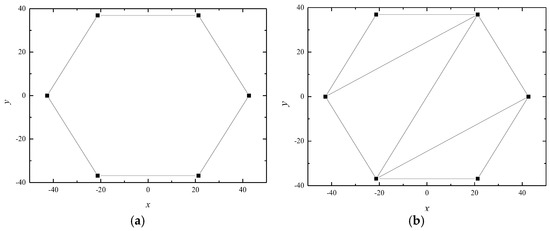
Figure 1. Geometric and triangular mesh models of a convex polygon. (a) Geometric model. (b) Triangular mesh model.

For concave polygons, if only the Delaunay triangulation algorithm or the sequential successive method is used, it will result in wrong sectioning results. In Figure 2a, simply connecting points i, j, and k will result in the mesh containing non-polygonal parts; as shown in Figure 2b, $△ijk$ is the correct triangular patch, while $△i^{\prime }{j}^{\prime }{k}^{\prime }$ is located in the outside of the polygon, which is the wrong triangular patch. Therefore, the following two conditions are required to form the correct triangular patch: the currently formed triangular patch does not contain any other point inside; if the polygons are sorted counterclockwise, the modulus length of the vector product of the vectors $\overrightarrow{ij}$ and $\overrightarrow{ik}$ of the currently formed triangle $△ijk$ is greater than 0 (or the modulus of the product of the vectors is less than 0 if the polygons are sorted clockwise).

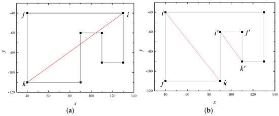
Figure 2. The triangulation of a concave polygon using the Delaunay triangulation algorithm. (a) Error 1. (b) Error 2.

Since the 2D cross-section of the horn antenna is an arbitrary polygon, we need to optimize the Delaunay triangulation algorithm to handle the triangulation of arbitrary polygons. The optimized triangulation algorithm is as follows: firstly, determine whether all the vertices are ordered clockwise or counterclockwise (if the area calculated from the vertex order is greater than 0, the order is counterclockwise; otherwise, it is clockwise). Secondly, when the number of remaining vertices is greater than four, determine whether $△ijk$ can form the correct triangular mesh (satisfying the above two conditions). If a correct triangular mesh can be formed, save the vertices of the triangle and remove vertex j from the vertex set, and proceed to the triangulation of the next mesh; otherwise, all vertices are shifted one position backward. Finally, when the remaining number of vertices is less than or equal to three, the process ends.

According to the optimized triangulation algorithm for the polygon in Figure 2, the result is shown in Figure 3a, which shows that the optimized triangulation algorithm can correctly handle the triangular mesh of concave polygons.

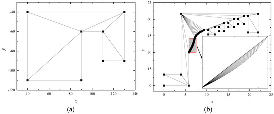
Figure 3. The triangulation of a concave polygon using the optimized triangulation algorithm. (a) A simple model. (b) A complex model.

3.2. The Algorithm for Transforming Triangular Meshes into BOR–FDTD Computational Meshes

Section 3.1 mainly implements the creation of triangular meshes for arbitrary polygons. In this section, the projection intersection method is used to transform the generated triangular mesh data into the BOR–FDTD computational model required for the analysis.

3.2.1. The Fast Modeling Method for Projection Intersection of Complex 3D Targets

For the projection intersection algorithm of complex 3D targets, firstly, the vertex data of all triangular surface meshes of the computational target are obtained and the maximum and minimum values of all vertices in the x, y, and z directions are solved: this range is the target region of the FDTD computational model. Subsequently, the target region is discretized by meshing based on the discrete sizes in the three directions. Finally, the relationship between the grid lines and the triangular mesh is judged.

As shown in Figure 4, the steps for judging the relationship between the FDTD mesh lines and the target are as follows. For any triangular mesh on the target surface the process is as follows [19]: firstly, the coordinate range of the current triangular mesh in the x and y directions is determined; then, in that range each grid line parallel to z is used to intersect the triangular mesh and the intersection coordinates are derived; finally, the intersection point is judged about the triangular surface mesh, and if it is within the triangular surface element the point is retained and assigned a medium number, as shown in Figure 5. According to this method, the projected intersections are carried out in the x, y, and z directions, respectively. Ultimately, the complex 3D target FDTD computational model can be obtained.

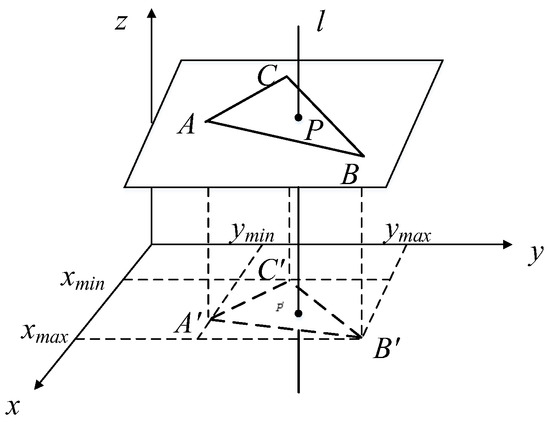
Figure 4. Intersection of the arbitrary spatial triangular mesh and FDTD grid lines.

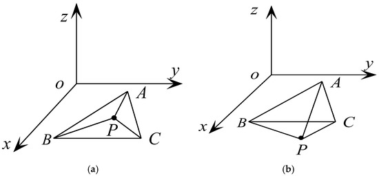
Figure 5. The relationship between intersection point P and a triangular mesh. (a) The intersection point is within the triangular mesh. (b) The intersection point is not within the triangular mesh.

The specific algorithm for determining the relationship between the intersection point $P$ and a triangular mesh is as follows. As shown in Figure 5, the vectors formed by the vertices $A$, $B$, $C$, and the intersection point $P$ are $\overrightarrow{PA}$, $\overrightarrow{PB}$, and $\overrightarrow{PC}$. The three vectors are cross-multiplied sequentially ($\overrightarrow{PA}\times \overrightarrow{PB}$, $\overrightarrow{PB}\times \overrightarrow{PC}$, and $\overrightarrow{PC}\times \overrightarrow{PA}$). If the three results have the same sign, then the intersection point $P$ is located inside $△ABC$.

3.2.2. The Projection Intersection Method for Fast Modeling of Complex 2D Rotationally Symmetric Targets

In this paper, the projective intersection method for 3D complex targets is drawn upon to model the 2D FDTD of a horn antenna cross-section. The projective intersection algorithm in 3D can deal with the projective intersection of any triangular surface mesh in space, and the 3D space is directly degraded to a 2D plane. In the $\rho -z$ plane, the coordinate ranges of the triangular mesh data in the $\rho$ and z directions are firstly obtained, and then the triangular meshes of the target are intersected with each line parallel to $\phi$; the coordinates of the intersection point are found, and it is judged whether these points are located within the triangular meshes. Finally, the BOR–FDTD computational model of the horn antenna cross-section is obtained.

3.3. Validation of the Adaptability of the Modeling Approach for Multi-Medium Situations

Based on the above algorithm, FDTD models can be established for any horn cross-section model. To verify the correctness of this algorithm, the established BOR–FDTD mesh computational models for both single-medium and multi-medium scenarios are presented. Figure 6 and Figure 7 show the geometric models and BOR–FDTD computational mesh models of different horns, where the different colors represent the different media. The results indicate that the optimized modeling method can handle the triangular mesh of arbitrarily complex polygonal shapes and the establishment of BOR–FDTD computational models.

Figure 6. Complex polygon with curves. (a) Geometric model. (b) FDTD mesh model.

Figure 7. Multi−medium model. (a) Geometric model. (b) FDTD mesh model.

4. Method Efficiency and Correctness Verification

The 3D model and cross-sectional model of a typical smooth-walled horn antenna is shown in Figure 8, with an overall length of the horn $L=55.6635 \mathrm{mm}$, radius of the horn inlet $R_{in}=8.85 \mathrm{mm}$, radius of the horn outlet $R_{out}=25.4072 \mathrm{mm}$, and wall thickness $d=3 \mathrm{mm}$. The feed mode is $T{E}_{11}$ mode.

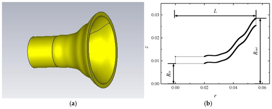
Figure 8. A typical smooth−walled horn antenna. (a) Three−dimensional model. (b) Cross−sectional model.

The model of Figure 8b was processed using the mesh generation algorithm of this paper and the built-in functions of MATLAB, respectively, and the cross-section model was divided into two sizes of FDTD mesh models, as shown in Table 1.

Table 1. Modeling efficiency tests.

Computing Region	Method	Calculation Time/s	Speed Ratio (Presented Method /MATLAB)
$330\times 648$	Presented method	0.004797	6.78%
	Built-in functions of MATLAB	0.070717
$1051\times 2071$	Presented method	0.014652	2.6%
	Built-in functions of MATLAB	0.554065

As can be seen from Table 1, for the case where the computational mesh size is $330\times 648$, the modeling time using the method proposed in this paper is only 6.78% of that required by the built-in functions in MATLAB 2017, effectively illustrating the efficiency of this modeling approach. As the grid size increases, the speed advantage of the method of this paper becomes even more pronounced.

The radiation patterns of the horn antenna were calculated using both the algorithm presented in this paper and the commercial software CST 2021 at frequencies of 18.2 GHz and 28 GHz, with the results displayed in Figure 9. A comparison of the computation times is provided in Table 2.

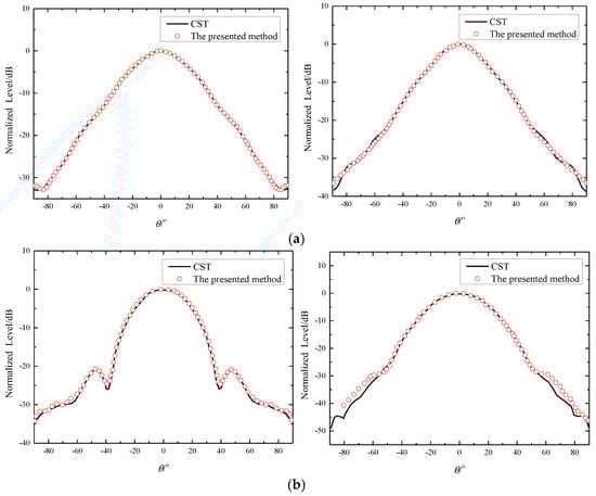
Figure 9. Radiation patterns of the E−plane and H−plane of the smooth−walled horn antenna. (a) 18.2 GHz. (b) 28 GHz.

Table 2. Comparison of computation times between the method presented in this paper and the commercial software CST.

Frequency/GHz	Calculation Time Consumed by Presented Method/s	Calculation Time Consumed by CST/s	Speed Ratio (Presented Method/CST)
18.2	72.4	231	31.3%
28	63.7	247	25.8%

As shown in Figure 9, the radiation patterns obtained from the presented method and the commercial software CST at two different frequencies demonstrate that as the frequency increases, the main lobe width decreases, while the number of side lobes increases. This indicates that the simulation results from the BOR−FDTD method align closely with those from CST, thus validating the correctness of the proposed algorithm. Additionally, in terms of computational efficiency, the BOR−FDTD method shows a significant advantage. According to Table 2, the calculation time consumed by the proposed method is approximately 32% of the simulation time of CST, resulting in a substantial reduction in computation time.

5. Conclusions

In this paper, a fast modeling method for rotationally symmetric structures is proposed based on the body-of-revolution finite-difference time-domain method, the Delaunay triangulation algorithm, and the projection intersection method. This approach is capable of handling arbitrary models for both single-medium and multi-medium scenarios, enabling the establishment of computational models for horn feeds and facilitating fast computations for rotational structures with a high modeling and computational efficiency.

References

- Ozdemir, C.; Yilmaz, B.; Keceli, S.I.; Lezki, H.; Sutcuoglu, O. Ultra Wide Band horn antenna design for Ground Penetrating Radar: A feeder practice. In Proceedings of the 2014 15th International Radar Symposium (IRS), Gdansk, Poland, 16–18 June 2014; pp. 1–4. [Google Scholar]
- Pliushch, O.; Kravchenko, Y.; Zhurakovskyi, B.; Savchenko, A.; Tyshchenko, M.; Salkutsan, S. Studying antenna-feeder matching effects with help of computer simulation model. In Proceedings of the 2022 IEEE 4th International Conference on Advanced Trends in Information Theory (ATIT), Kyiv, Ukraine, 15–17 December 2022; pp. 259–263. [Google Scholar]
- Ridho, S.; Apriono, C.; Yuli Zulkifli, F.; Tjipto Rahardjo, E. Design of corrugated horn antenna with wire medium addition as parabolic feeder for Ku-band Very Small Aperture Terminal (VSAT) application. In Proceedings of the 2020 International Conference on Radar, Antenna, Microwave, Electronics, and Telecommunications (ICRAMET), Tangerang, Indonesia, 18–20 November 2020; pp. 163–166. [Google Scholar]
- Jacobs, O.B.; Odendaal, J.W.; Joubert, J. Elliptically shaped quad-ridge horn antennas as feed for a reflector. IEEE Antennas Wireless Propag. Lett. 2011, 10, 756–759. [Google Scholar] [CrossRef]
- Thomas, B. A review of the early developments of circular-aperture hybrid-mode corrugated horns. IEEE Trans. Antennas Propag. 1986, 34, 930–935. [Google Scholar] [CrossRef]
- Rieter, J.M.; Arndt, F. Efficient hybrid boundary contour mode-matching technique for the accurate full-wave analysis of circular horn antennas including the outer wall geometry. IEEE Trans. Antennas Propag. 1997, 45, 568–570. [Google Scholar] [CrossRef]
- Adam, J.-P.; Romier, M. Design approach for multiband horn antennas mixing multimode and hybrid mode operation. IEEE Trans. Antennas Propag. 2017, 65, 358–364. [Google Scholar] [CrossRef]
- Chinn, G.C.; Epp, L.W.; Hoppe, J.D. A hybrid finite-element method for axisymmetric waveguide-fed horns. IEEE Trans. Antennas Propag. 1996, 44, 280–285. [Google Scholar] [CrossRef]
- Venkatarayalu, N.V.; Chen, C.-C.; Teixeira, F.L.; Lee, R. Numerical modeling of ultrawide-band dielectric horn antennas using FDTD. IEEE Trans. Antennas Propag. 2004, 52, 1318–1323. [Google Scholar] [CrossRef]
- Zang, S.R.; Bergmann, J.R. Analysis of omnidirectional dual-reflector antenna and feeding horn using method of moments. IEEE Trans. Antennas Propag. 2014, 62, 1534–1538. [Google Scholar] [CrossRef]
- Chen, Y.; Mittra, R.; Harms, P. Finite-difference Time-domain algorithm for solving Maxwell’s equations in rotationally symmetric geometries. IEEE Trans. Microw. Theory Tech. 1996, 44, 832–839. [Google Scholar] [CrossRef]
- Rolland, A.; Ettorre, M.; Drissi, M.; Coq, L.L.; Sauleau, R. Optimization of reduced-size smooth-walled conical horns using bor-FDTD and genetic algorithm. IEEE Trans. Antennas Propag. 2010, 58, 3094–3100. [Google Scholar] [CrossRef]
- Wang, Y.-G.; Chen, B.; Chen, H.-L.; Xiong, R. An unconditionally stable one-step leapfrog ADI-BOR-FDTD method. IEEE Antennas Wireless Propag. Lett. 2013, 12, 647–650. [Google Scholar] [CrossRef]
- Shenton, D.; Cendes, Z. Three-Dimensional finite element mesh generation using delaunay tesselation. IEEE Trans. Magn. 1985, 21, 2535–2538. [Google Scholar] [CrossRef]
- Elshakhs, Y.S.; Deliparaschos, K.M.; Charalambous, T.; Oliva, G.; Zolotas, A. A Comprehensive Survey on Delaunay Triangulation: Applications, Algorithms, and Implementations Over CPUs, GPUs, and FPGAs. IEEE Access 2024, 12, 12562–12585. [Google Scholar] [CrossRef]
- Shinan, Z.; Jiachuan, Y.; Jun, P. Research on algorithm of target triangles fast locating in Delaunay triangulation. In Proceedings of the 2020 IEEE International Conference on Artificial Intelligence and Information Systems (ICAIIS), Dalian, China, 20–22 March 2020; pp. 802–805. [Google Scholar]
- Su, T.; Liu, Y.J.; Yu, W.H.; Mittra, R. A conformal mesh-generating technique for the conformal finite-difference time-domain (CFDTD) method. IEEE Antennas Propag. Mag. 2004, 46, 37–49. [Google Scholar]
- Zhong, B.; Feng, J.; Fang, M.; Huang, Z. A structured meshing approach for FDTD method. In Proceedings of the 2024 IEEE 7th International Conference on Electronic Information and Communication Technology (ICEICT), Xi’an, China, 31 July–2 August 2024; pp. 1232–1235. [Google Scholar]
- Srisukh, Y.; Nehrbass, J.; Teixeira, F.L.; Lee, R. An approach for automatic grid generation in three-dimensional FDTD simulation of complex geometries. IEEE Antennas Propag. Mag. 2002, 44, 75–80. [Google Scholar] [CrossRef]
Disclaimer/Publisher’s Note: The statements, opinions and data contained in all publications are solely those of the individual author(s) and contributor(s) and not of MDPI and/or the editor(s). MDPI and/or the editor(s) disclaim responsibility for any injury to people or property resulting from any ideas, methods, instructions or products referred to in the content. |
© 2024 by the authors. Licensee MDPI, Basel, Switzerland. This article is an open access article distributed under the terms and conditions of the Creative Commons Attribution (CC BY) license (https://creativecommons.org/licenses/by/4.0/).