Abstract
This paper introduces a model that predicts four common smartphone-holding postures, aiming to enhance user interface adaptability. It is unique in being completely independent of platform and hardware, utilizing the inertial measurement unit (IMU) for real-time posture detection based on sensor data collected around tap gestures. The model identifies whether the user is holding and operating the smartphone with one hand or using both hands in different configurations. For model training and validation, sensor time series data undergo extensive feature extraction, including statistical, frequency, magnitude, and wavelet analyses. These features are incorporated into 74 distinct sets, tested across various machine learning frameworks—k-nearest neighbors (KNN), support vector machine (SVM), and random forest (RF)—and evaluated for their effectiveness using metrics such as cross-validation scores, test accuracy, Kappa statistics, confusion matrices, and ROC curves. The optimized model demonstrates a high degree of accuracy, successfully predicting the holding hand with a 95.7% success rate. This approach highlights the potential of leveraging sensor data to improve mobile user experiences by adapting interfaces to natural user interactions.
1. Introduction
People interact with their mobile devices in many different ways. This makes designing user interfaces challenging as the interface will only suit one type of group while others may struggle because of the way they hold their smartphones. If the smartphone were aware of how the user currently interacts with the device, the user interface and general handling of the mobile device could autonomously adapt to the specific usage context in real time.
In 2013, Steven Hoober conducted a survey by observing 1333 people in public places (e.g., streets, airports, bus stops, cafés, trains, and buses) to analyze how they interact with their smartphones [1]. People nowadays use their mobile devices in many different scenarios (for example, while walking, riding a bus, or standing still), and adapt their grip on the smartphone accordingly. Hoober’s observations revealed that 49% of people hold their phone in one hand, 36% hold it cradled (one hand holding the phone, one hand interacting with the touchscreen—either with the thumb or the index finger), and 15% use two hands.
Looking at one-handed interactions, interestingly, only 67% of people use their right hand. In contrast, 33% use their left hand, which does not correlate with the number of left-handed people in the general population (about 10%) [2]. This observation shows that right-handed people are likely to operate their mobile devices from time to time to free up their dominant hand for other tasks. Considering this, user interface (UI) designs should not only be focused on right-handed people as nearly 1/3 of one-handed interactions are done with the left hand.
After studying one-handed interactions, two common ways of holding a phone with one hand can be identified:
- Thumb on the display, with the other four fingers on the side.
- Thumb on the display, pinkie on the bottom, with the other three fingers on the side.
These differences result in varying screen coverage, e.g., with the pinkie supporting the bottom, it is harder to reach the top left corner, while the other holding posture makes it tough to reach the bottom right corner, as illustrated in Figure 1.
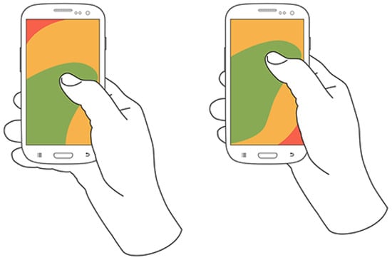
Figure 1.
Thumb coverage during one-handed interaction with the right thumb, showing different holding postures [1].
Looking at two-handed interactions with both thumbs, people use this method mostly for gaming, video consumption, and typing on the keyboard.
It should be noted that smartphones are generally becoming larger. For example, Apple’s iPhone began with a 4-inch display in 2013 (iPhone 5s) and expanded to a 6.7-inch display by 2022 with the iPhone 13 Pro Max.
This makes one-handed interactions with the mobile device harder. Apple, for example, offers a one-handed mode where a swipe down from the bottom of the display shifts the entire UI downward. Without this feature, the classic back button in the top-left corner of the screen would be nearly impossible to reach for a user with an average-sized hand on an iPhone 13 Pro Max. However, this solution requires active user input, which is suboptimal.
In this paper, we propose a method to detect how the user interacts with the smartphone at runtime in the background, allowing UI designers to utilize this information when designing interfaces. A practical example is the zoom operation in a maps application: The standard method is to pinch with two fingers, which can be challenging on a large smartphone operated with one hand. In this case, the zoom function could be adjusted to use a long press on the touchscreen, followed by an upward or downward swipe while still pressing, to zoom in and out—an interaction easily performed with one hand. Furthermore, posture recognition can help prevent unintentional touches on the screen. One-handed operation on large smartphones is often challenging, especially when trying to tap small UI buttons, which may result in accidental touches and unintended actions. A clever UI design can consider the information of the holding posture to counteract unintentional touches, for example, by expanding the surface of buttons to make them easier to reach. Another use case involves gesture-based interactions. The smartphone can also recognize certain holding postures as triggers for specific gestures. For instance, a double-tap gesture while holding the phone with one hand can be used to take screenshots, while a long press followed by sliding the finger up or down can be interpreted as a zoom gesture. Finally, knowing the holding posture can also enable safety features. Smartphones today can detect whether they are being used while stationary, walking, riding, or driving. In combination with this information, an app can disable a subset of features in the application depending on where (and how) the user operates the smartphone. For example, if the user is driving a car and the app detects that the smartphone is held with one hand, the application can disable certain features like texting or social media notifications to reduce distractions, as using the smartphone while driving is generally illegal in most countries.
To achieve this recognition, a machine learning (ML) model is trained with the sensor data from the inertial measurement unit (IMU) of a smartphone. The dataset used for the training was recorded with different participants of different sex and age while interacting with the smartphone.
This study offers a novel contribution by introducing a real-time, platform-agnostic model for smartphone posture recognition that adapts based on sensor data, without relying on specific hardware configurations or pre-defined gestures. This unique approach leverages IMU sensor readings to predict holding postures with high accuracy, distinguishing it from existing models that typically rely on touchscreen interactions or require supplementary sensors. This capability has significant implications for adaptive UIs that can automatically adjust to a user’s natural interactions, enhancing both accessibility and user satisfaction across various smartphone tasks and contexts.
The rest of this paper is structured as follows: Section 2 summarizes and discusses relevant related work. Section 3 presents a data-recording session and focuses on the IMU data used to train the ML models. Section 4 discusses feature extraction, analysis, and selection to optimize the feature set. Section 5 focuses on model selection and hyperparameter tuning. The final results and a detailed evaluation are presented in Section 6. Section 7 presents our summary and conclusion.
2. Related Work
Detecting the holding posture of a mobile device is an active field of study with a variety of approaches. Some studies utilize external hardware, some rely on specific patterns during the unlocking process, and others require touchscreen interactions such as tapping or swiping.
2.1. Prototype with External Hardware
Wimmer et al. [3] utilized capacitive sensors in their prototype “HandSense” to determine which hand holds the device, achieving an accuracy of 80%. For this task, they defined six different holding postures based on how the user touches the frame of the prototype, thereby interacting with the capacitive sensors in distinct ways. They placed two capacitive sensors on each of the longer sides of the prototype and used a sample rate of 25 Hz.
The capacitive sensors can be used to estimate the thickness of objects, as bigger objects will return higher sensor readings than smaller ones. Wimmer and Boring utilized this property to differentiate whether the fingers or the ball of the thumb were touching the sensor. This information is then used within a state machine to determine the holding posture, For example, if the sensor reading at the bottom of the right side is higher than at the bottom of the left side, and the sum of the sensor readings on the left side is smaller than on the right side, the smartphone is most likely held in the right hand. For more robustness, they implemented a mechanism that verifies the state if it is recognized five consecutive times. In their user study, they found that successful detection of the holding posture occurs within approximately 600 to 700 milliseconds.
2.2. Focus on the Unlocking Process
Löchtefeld et al. [4] primarily focused on the characteristics during the unlocking process of a smartphone in order to predict the holding posture. In their user study, they used an LG Google Nexus 5 smartphone with which the participants were asked to perform three different unlocking mechanisms with three different holding postures, respectively: right-handed, left-handed, and two-handed. During the unlocking process, they recorded accelerometer data, device orientation, and touchpoints of the interaction. To compare these time series of varying lengths, they applied dynamic time warping (DTW). Since a support vector machine (SVM) did not improve the results compared to the k-nearest neighbors (kNN) model and would be computationally more expensive, they opted for the kNN model, achieving an accuracy of 98.51%.
A different approach was presented by Avery et al. [5]. They detected the holding posture prior to the first touchscreen interaction by using the inertial measurement unit (IMU) data and DTW. Their user study was conducted using a Nexus 5 smartphone, which recorded accelerometer, gravity, and orientation data between power-on and unlock, with the phone lying face-down on the table at the beginning of each experiment. Participants picked up the smartphone and were asked to perform a swipe-to-unlock procedure using a slider that was randomly placed in five different locations, with ten combinations of position and swipe direction. Four holding postures were defined for the experiment, which were also applied in the study presented in this paper (see Figure 2). Their holding posture recognition model only achieved an accuracy of 58.55%; hence, they switched to a hand detection model to differentiate between the left and right hands. That model had an overall accuracy of 83.6%, which means the wrong hand was predicted roughly one out of every seven times. Also, the authors examined a per-user model, which required data from each user, possibly with a system alert asking for the current holding hand. In their study, they found that only two training samples for each user were enough for a reasonable classification.
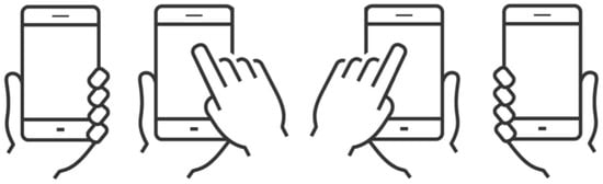
Figure 2.
Defined holding postures used for the experiment, from left to right: left-single, left-double, right-double, and right-single [5].
2.3. Utilizing Touchscreen Interactions
Goel et al. [6] presented their prototype “GripSense”, used to detect the holding posture (left/right thumb, index finger) after a sequence of touchscreen interactions (tapping, swiping). Their model combines gyroscope, accelerometer, and touchscreen data. Fortunately, Android devices provide the touch size of an interaction on the touchscreen. Using this information, they engineered three features based on some basic assumptions:
- Rotation: The gyroscope was sampled at 1000 Hz to capture the device’s rotation as accurately as possible. The researchers determined that rotation is greater at the top of the screen than at the bottom during one-handed interactions. Thus, this variation can be used to indicate whether the user is operating the smartphone with one hand or two.
- Touch size: By analyzing the size and change of touch interactions based on their position on the touchscreen, researchers extracted information about whether the device was being used with a thumb or index finger. They assumed that touch interactions with the thumb at the top of the device would result in a larger touch size compared to interactions near the center.
- Shape of the swipe: While swiping with the index finger typically results in a straight line on the touchscreen, swiping with either thumb creates a distinct arc to the right or left due to the anatomy of the hand. This arc can be analyzed to determine whether the user is holding the smartphone in their left or right hand.
The final decision to detect the holding posture was made by a state machine that combined these three features using a majority vote. If swipe gestures were absent, a decision was made only if the two remaining features agreed; otherwise, the model yielded no holding posture. After about five interactions, they were able to detect the holding posture with an accuracy of 81.11% when swipe gestures (and, therefore, the third heuristic) were not included. In comparison, they achieved an accuracy of 87.4% after only four interactions when swipe gestures were included.
Goel et al. [7] extended their previous work “GripSense” to focus on posture recognition during keyboard typing to adjust an adaptive keyboard design. Therefore, they used the model from their previous work and also included typing with both thumbs as a gesture. For this holding posture, they analyzed the time elapsed between two taps and the touch size, based on the assumption that it takes longer to move from one side of the touchscreen to the other during one-handed interaction compared to two-handed typing with both thumbs. With this extension, they were able to differentiate between four holding postures with an accuracy of 89.7% after an average of 4.9 touchscreen interactions. In their user study, they combined this model with a language model to predict the most likely next key press and adjust the keyboard accordingly, resulting in a 20.6% reduction in typing errors.
Park and Ogawa [8] presented a similar idea to “GripSense” by analyzing each touch interaction at runtime to extract different holding postures but used quite a different methodology. They extracted gyroscope and accelerometer data at 50 Hz, along with touchscreen information (size and location) for each interaction, capturing data 0.2 s before and after each tap gesture. The data were preprocessed using a fast Fourier transform (FFT) to extract meaningful features as input for their SVM model. In their user study with six participants, conducted on a Samsung Galaxy Note 3, they achieved an accuracy of 87.7% in differentiating between all five holding postures, and an accuracy of 94.4% for four postures, excluding the two-handed posture with both thumbs.
2.4. Differences from This Paper and the New Approach
Summing up these approaches, some existing approaches require external sensors, some focus solely on the action of grabbing the phone and unlocking it, while others detect the holding posture during actual user interactions but need a certain number of interactions in order to work properly.
In contrast to the approaches mentioned above, the method proposed in this study operates independently of external sensors, does not focus only on the unlocking process of a smartphone, and detects holding posture changes during the usage of an application at runtime. The majority of this paper will focus on comparing different machine learning approaches, feature processing methods, and feature selection techniques to identify the model best suited for this task. To ensure a generic model that can be used on both Android and iOS devices, only IMU data and touch interaction coordinates will be utilized, as these data points are available on nearly all smartphones today. The prediction is made solely by the model, without relying on pre-calculated heuristics based on phone usage assumptions.
3. Data Recording and Visualization
To maintain control over the pipeline, a custom dataset was recorded specifically for this study, rather than using pre-existing data. This approach allowed us to experiment with different sensors, sampling frequencies, and recording conditions, instead of being constrained by a fixed dataset. The goal of the final model is to be platform- and hardware-independent, meaning that only sensor data available on most smartphones should be used. Notably, almost every mobile phone today has a built-in IMU.
Smartphones generally only use capacitive touchscreens now [9]. They consist of a conductor layer that can sense disturbances in the electrical field when a conductive object touches the touchscreen, for example, the finger. From that information, the positions (X and Y coordinates) can then be calculated.
The idea was to sample the IMU at 100 Hz and save a buffer in the background of a smartphone application. As soon as the user taps the touchscreen, the location of the interaction, as well as 0.5 s of IMU data before and after the interaction, are used for the decision-making of the model. That way, each axis of each sensor of the IMU contains exactly 100 data points. The orientation (yaw, pitch, and roll) is also fetched at 100 Hz from the IMU, if possible, otherwise, it is simply calculated. Each interaction, therefore, totals exactly 1202 data points.
- Accelerometer, gyroscope, magnetometer: 100 data points for each sensor (x-, y-, and z-axes).
- Orientation: 100 data points (yaw-, pitch-, roll-axis).
- Coordinates: 1 data point (x- and y-axes).
Considering both studies by Steven Hoober, mentioned in Section 1, as well as the approaches of related works, four holding postures appear to be the most relevant for everyday usage, as visualized in Figure 2: (i) left single-handed, (ii) left double (holding the smartphone in the left hand and interacting with the right hand), (iii) right double-handed (holding the smartphone in the right hand and interacting with the left hand), and (iv) right single-handed.
Data Visualization
In total, nine participants contributed to the final dataset (seven male, two female), between the ages of 23 and 58, all of them right-handed. This should not be too concerning. Right-handed individuals may use their smartphone with their non-dominant hand in certain situations, such as when their dominant hand is occupied—for example, holding the smartphone with their left hand while retrieving keys from their pocket with their right hand [1]. This indicates that non-dominant hand usage is a familiar interaction for participants, contributing to the reliability of the posture data collected. The dataset consists of 723 rows (samples) and 1204 columns (1202 features + username + holding posture). The target variable is nearly uniformly distributed, as seen in Figure 3a, while the participants tapped at different frequencies on the touchscreen, as visualized in Figure 3b.
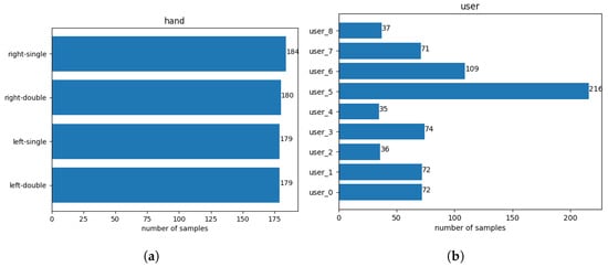
Figure 3.
(a) Number of samples for each holding posture in the dataset. (b) Number of samples each user contributed to the final dataset.
Next up, the location where the user touched the screen is labeled into nine different categories:
- Top row: left, middle, right.
- Middle row: left, middle, right.
- Bottom row: left, middle, right.
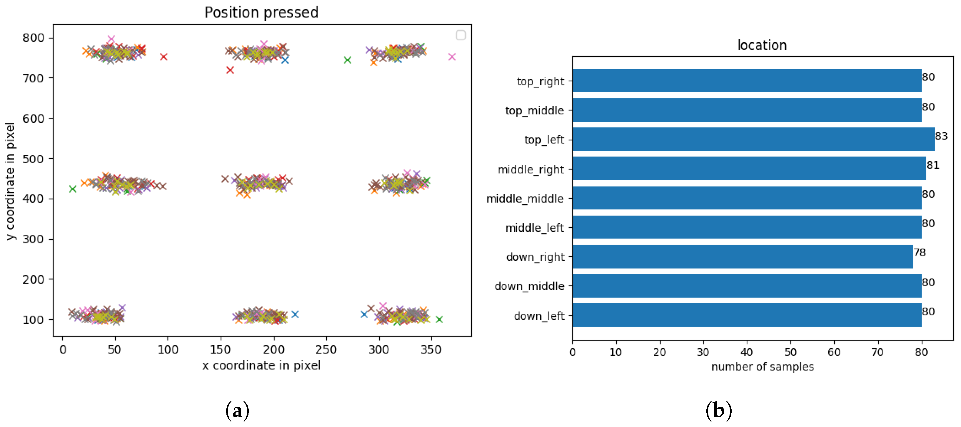
The number of samples per location can be seen in Figure 4 while Figure 4a visualizes the X and Y coordinates of all tap gestures in total.
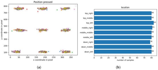
Figure 4.
(a) Actual X and Y coordinates of all tap gestures in the dataset. (b) Number of samples per location (dataset split into nine different locations categorized by the labels displayed in the app).
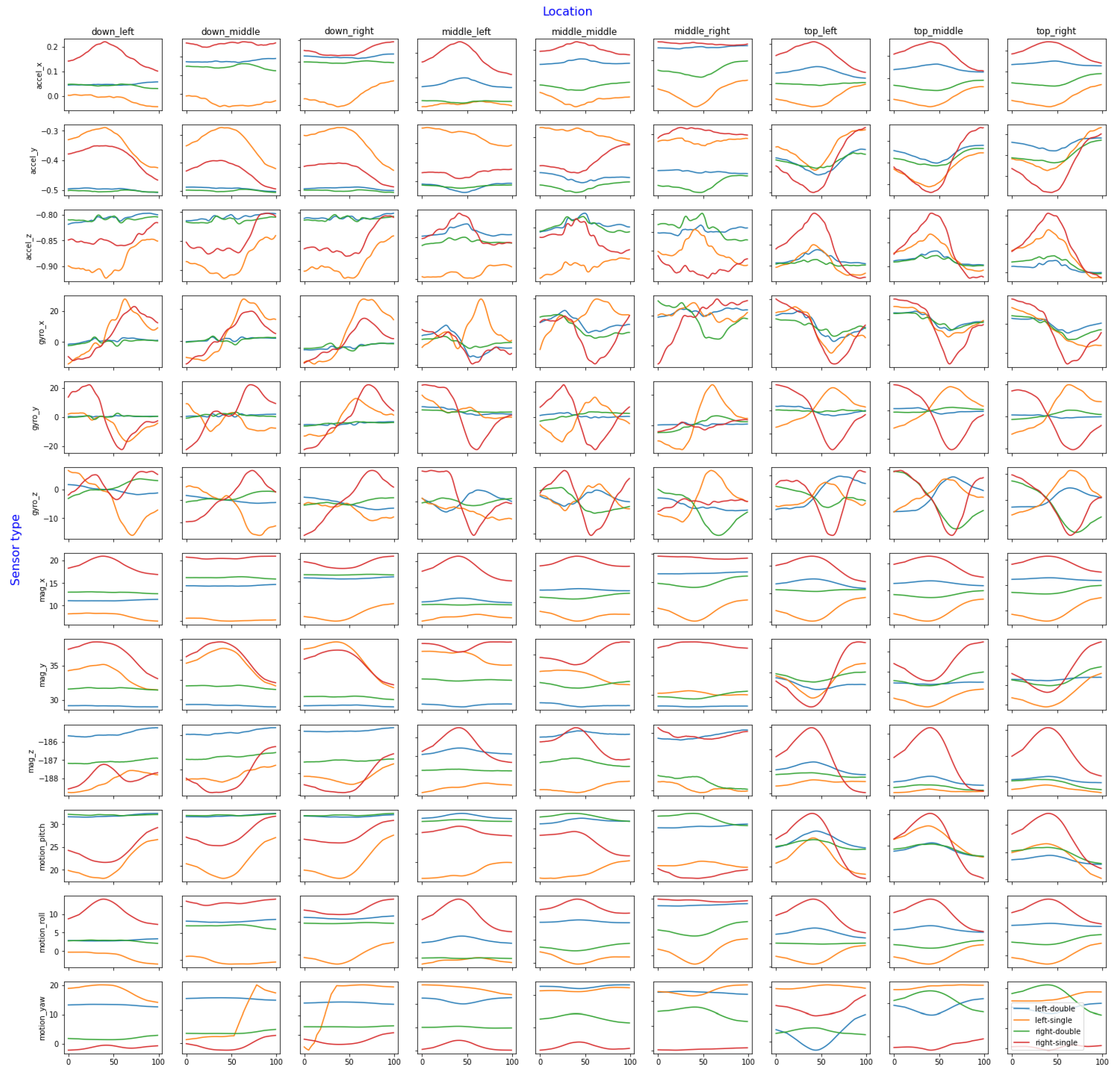
The whole dataset is visualized in Figure 5. The Y-axis consists of all different sensors and axes for each sensor while the X-axis contains the nine labeled locations where the users tapped the screen. These groupings are important, as different locations yield different sensor values. For example, using the smartphone right-handed and attempting to tap a button at the bottom-right corner of the phone often causes a slight rotation in the pitch axis, where the top of the smartphone will tilt down most of the time. On the other hand, trying to tap a button located at the top-left corner (such as the classic back button on an iPhone) also causes a pitch-axis rotation, but in this case, the top of the phone tilts upward (toward the user, toward the thumb). This movement can also be seen in other sensors, such as the gyroscope or accelerometer. For this reason, it is best to group the charts by sensor axis and location to determine whether the target variables are visually distinguishable. The figure shows every sensor and location; although some axes may be less important than others, it is still necessary to compare all the recorded data.
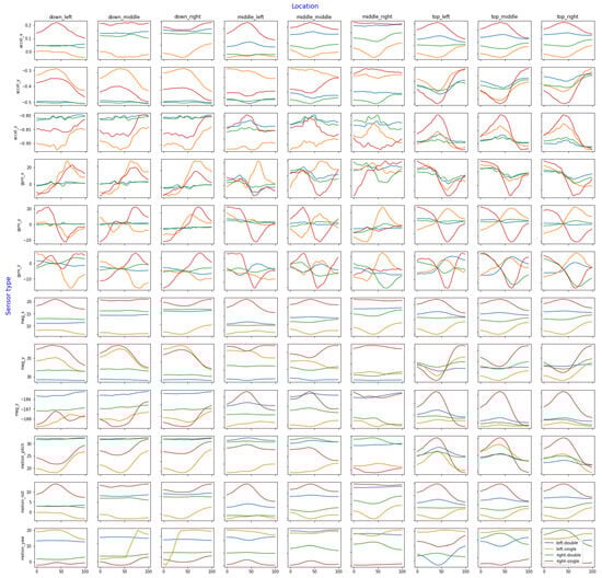
Figure 5.
The whole dataset visualized and grouped by sensor axis, location, and holding posture, with a rolling median filter and a window size of 25.
Finally, the use of a rolling median filter with a window size of 25 to analyze the data yields substantial improvements in data clarity and comprehension. Notably, the Y- and Z-axes of the gyroscope exhibit remarkable discriminatory capabilities in distinguishing between the four distinct holding postures, with each posture having a distinct pattern in these axes. These findings unveil insights into the potential of gyroscope data as viable data sources for posture classification.
The original dataset is augmented by 30%. Thus, the newly generated dataset contains 940 samples in total; of these, 77% of the samples are real-world samples and the remaining 23% samples are generated ones.
4. Data and Feature Preprocessing
Following data preparation and augmentation, we proceed with feature extraction. The raw dataset comprises 1202 features from four sensors (accelerometer, gyroscope, magnetometer, and orientation), with each sensor recording three axes (100 values per axis) and X-Y coordinates for tap gestures. Since the ML models do not inherently recognize dependencies between consecutive time series values, using the raw data may introduce unnecessary complexity and computational overhead. Nonetheless, this raw dataset serves as a baseline to evaluate model performance, allowing comparisons with the derived feature sets.
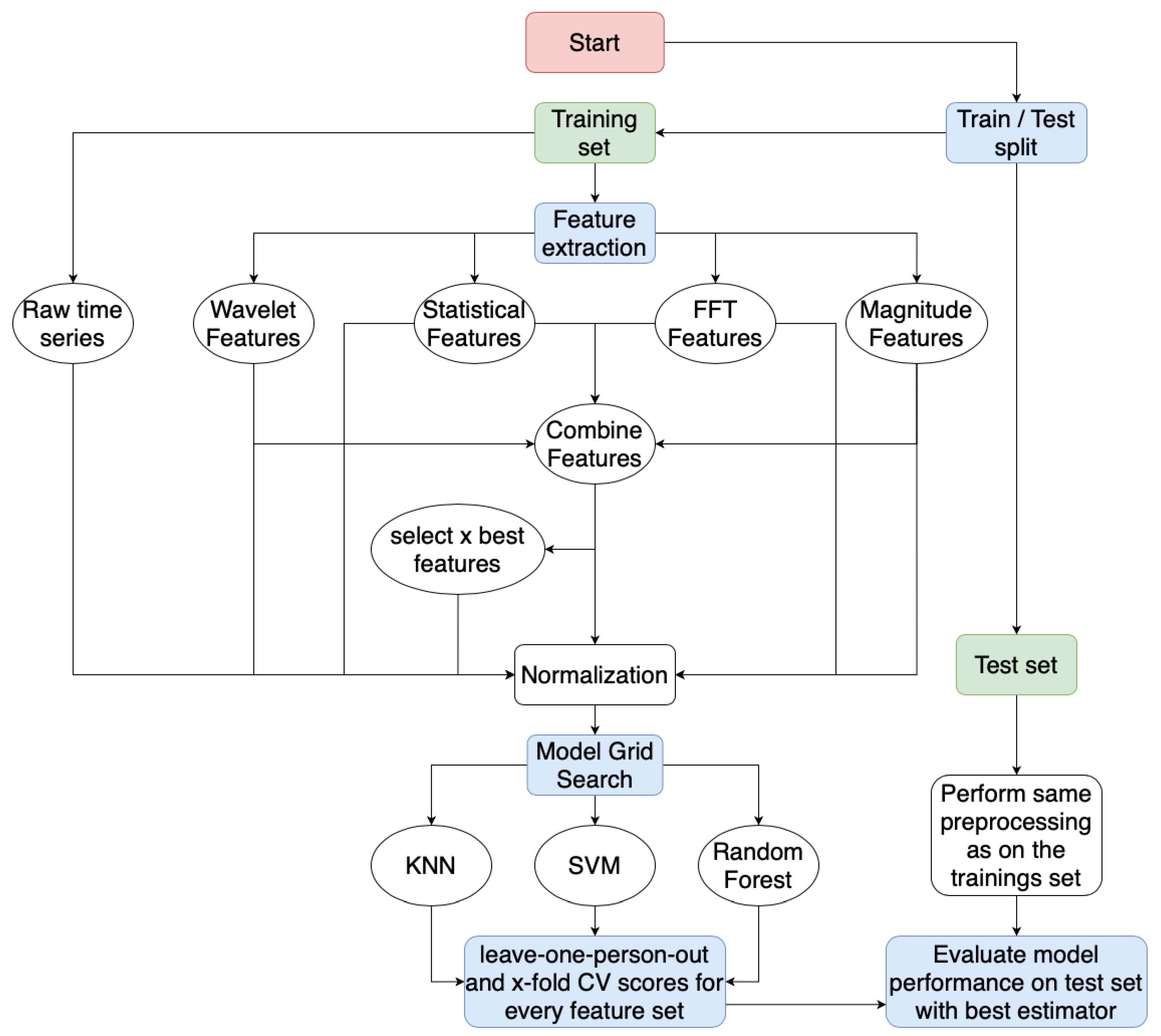
Various methods are available for extracting features from time series data, which can be categorized into time, frequency, and time-frequency domain features. The flowchart Figure 6 outlines the overall workflow, from the raw dataset through preprocessing (the primary focus of this chapter), model selection, and final evaluation.
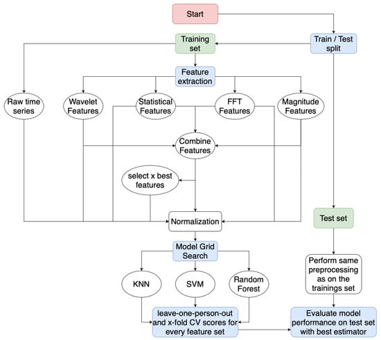
Figure 6.
Flowchart explaining the different steps from an unmodified dataset up to the final model evaluation.
The dataset is divided into training and test sets, typically with an 80/20 or 70/30 split, to ensure sufficient data for training while reserving a portion for performance evaluation on unseen data [10]. This ratio, inspired by the Pareto Principle, suggests that 80% of effects arise from 20% of causes [11], making it applicable to machine learning by reserving a subset for testing model generalizability. The next phase is the feature extraction process. In addition to the raw time series data, various features are extracted from the time, frequency, and time-frequency domains, and combined into a single feature set.
4.1. Feature Extraction
4.1.1. Time-Domain Features
The raw time series data can serve as time-domain features, but using unprocessed values is generally not recommended. Standardizing the data, typically by adjusting each feature to have a mean of 0 and a standard deviation of 1, improves model effectiveness [12]. This step is particularly important for models such as SVMs and linear models, which assume normalized features. Without standardization, features with high variance could dominate the objective function, impeding model learning. As a minimum preprocessing step, we applied StandardScaler from scikit-learn to achieve standardization.
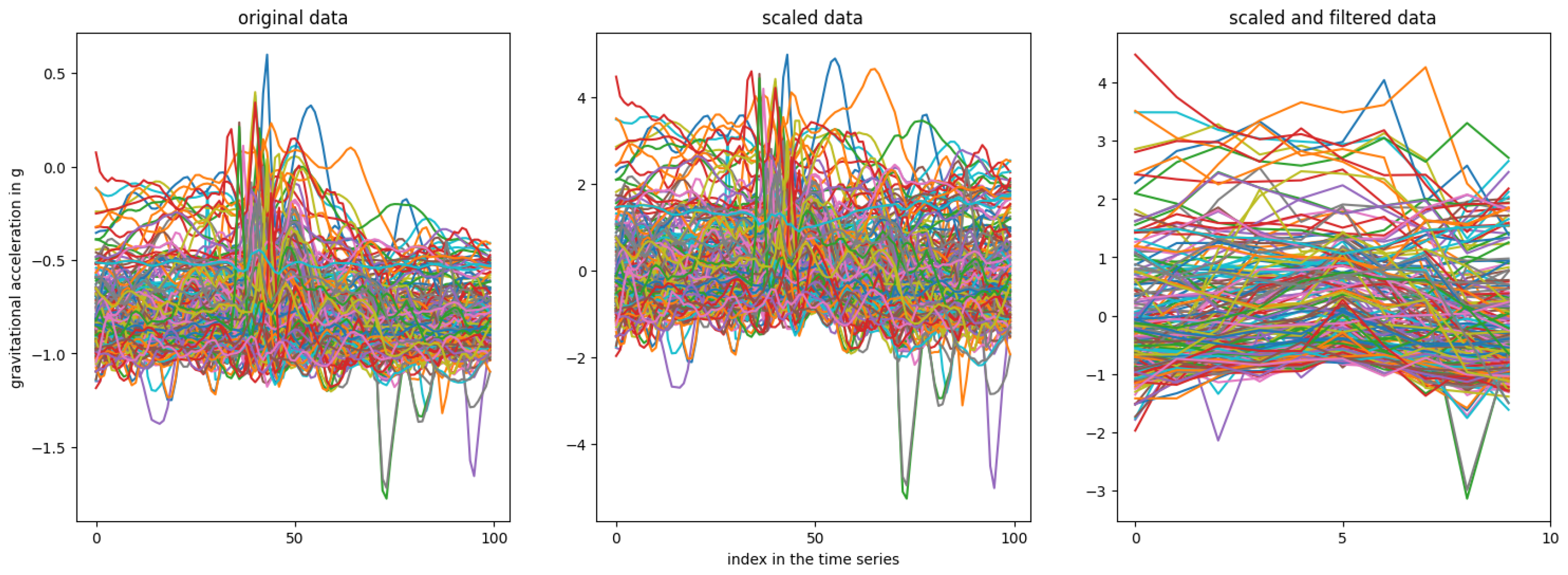
Using StandardScaler to scale a time series of 100 data points (one per feature) typically results in distinct mean and standard deviation values for each feature. However, due to the varying responses of each sensor axis based on holding posture and tap location Section 3, applying unique scaling factors for each feature could disrupt temporal dependencies. Thus, it is preferable to scale the entire time series with uniform mean and standard deviation values, even if this yields suboptimal scaling for individual features. Figure 7 illustrates the raw accelerometer z-axis compared to both scaled and scaled-filtered data, where a rolling mean filter with a window of 10 reduces the time series from 100 to 10 samples.
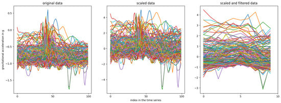
Figure 7.
Comparison of the raw time series data from the accelerometer’s Z-axis with the scaled time series data using a custom scaling implementation, as well as the scaled and filtered data.
As noted, this scaling approach may not yield precise mean and standard deviation values for each feature. However, by averaging the mean and standard deviation values across all columns (see Table 1), it is evident that both custom scaling and filtering methods produce a time series approximately centered at 0 with a standard deviation close to 1. The original time series had a mean of and a standard deviation of 0.19, highlighting the necessity of scaling. While StandardScaler may achieve slightly better values, this difference is likely negligible.

Table 1.
Mean and standard deviation value comparison for one raw time series (accelerometer z-axis) and different scaling/filtering implementations.
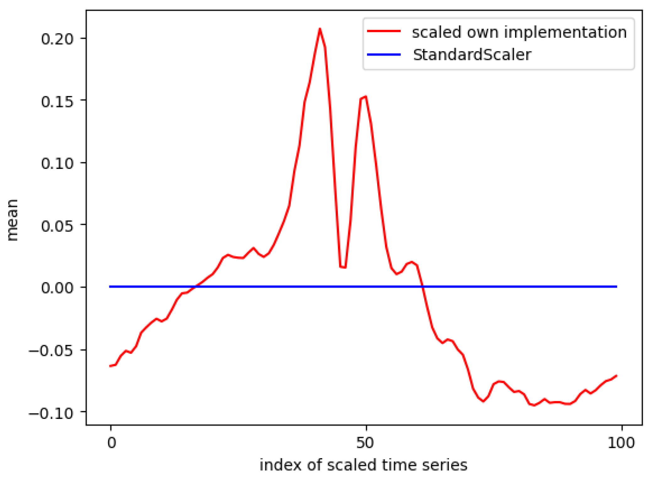
Analyzing the mean values across all columns reveals a notable difference between the custom implementation and StandardScaler. As shown in Figure 8, StandardScaler achieves a mean of 0 for each column, ensuring equal contribution from each feature to the ML model. In contrast, the custom method results in slight variations in mean values across columns, with notable spikes around tap gestures. These spikes suggest that features around the tap event are more influential, raising the question of whether sampling IMU data at 100 Hz for 0.5 s before and after a tap is necessary or if a shorter time window may suffice.

Figure 8.
Comparison of the mean values of a time series (accelerometer z-axis) after being scaled with different scaling implementations.
In addition to using scaled and filtered time series as time-domain features, various statistical features can be extracted for each sensor axis. Basic statistics include the mean, median, minimum, maximum, standard deviation, and variance, which can be calculated using Python’s NumPy package.
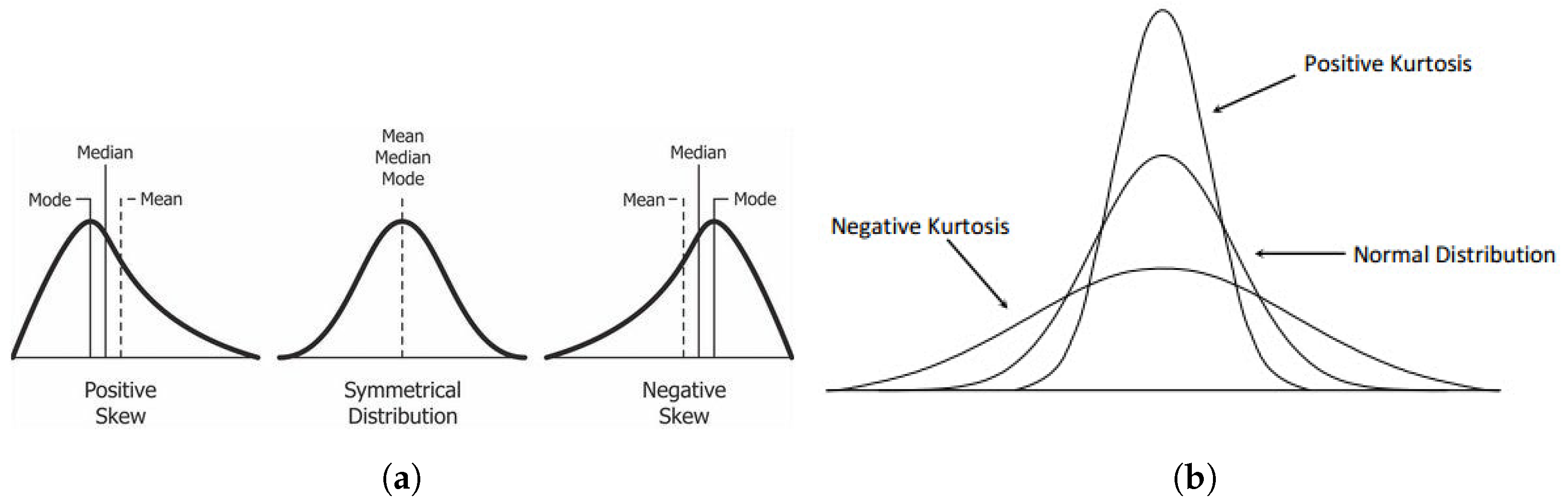
Skewness, which measures distribution asymmetry, can also be a feature. The scikit-learn package provides a method to compute skewness, where a value of 0 indicates normal distribution; positive skewness suggests left-sided concentration, while negative skewness indicates right-sided concentration (visualized in Figure 9a). Similarly, kurtosis describes tail heaviness relative to a normal distribution. A kurtosis of 0 suggests a normal distribution, positive kurtosis indicates heavier tails and negative kurtosis reflects lighter tails (see Figure 9b).
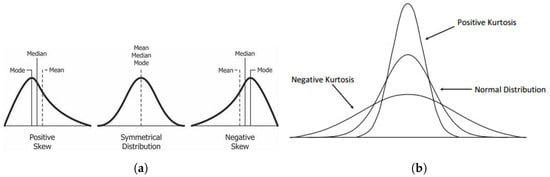
Figure 9.
(a) Visualization of positive and negative skewness in time series data [13]. (b) Comparison between positive and negative kurtosis [14].
Additional statistical features can be derived for each sensor axis, including the following:
- Interquartile range (IQR): Measures data spread between the 25th and 75th percentiles, offering robustness against outliers.
- Median absolute deviation (MAD): Quantifies dispersion with less sensitivity to outliers by calculating the median distance of values from the median.
- Peak to peak: The range between the maximum and minimum values in the time series.
- Integration: The area under the curve, calculated using the composite trapezoidal rule.
- Root mean square (RMS): The square root of the mean of squared values; useful as a statistical measure.
- Number of peaks: The number of data points exceeding a specified threshold (e.g., mean value).
Additionally, features can be extracted from the magnitude, which combines the three sensor axes, thereby losing orientation information but capturing overall motion intensity. The L2 norm (magnitude) is calculated as follows [15]:
Further statistics, such as mean, maximum, minimum, variance, standard deviation, and the number of peaks, are then derived from this magnitude.
4.1.2. Frequency Domain Features
Beyond the time-domain analysis, features can also be extracted from the frequency domain. This requires applying a Fourier transform to the time series, converting it to the frequency domain. For discrete time-series data, the discrete Fourier transform (DFT) is used, represented as follows:
where is the Fourier-transformed data, is the original time-domain data, and N is the sample count. The fast Fourier transform (FFT) is a common, efficient algorithm used to compute the DFT.
Post-transformation, the magnitude’s mean and standard deviations are extracted as features [16]. Additionally, the phase of the complex numbers in the transformed signal provides further insights; its mean and standard deviation are also used as features [17].
4.1.3. Time-Frequency Domain Features
Feature extraction from time series data reveals underlying patterns, but solely using time-domain features captures only temporal aspects, missing key frequency information. Conversely, Fourier transforms provide frequency details but lose temporal context. Wavelet transforms address this balance by decomposing a signal into multiple frequency-specific levels, combining both time and frequency insights [18,19]. Standard time-series analysis lacks frequency details, while Fourier transforms capture frequency without time context. Gábor analysis [19] offers both through short-time Fourier transforms in specific time windows. Wavelet transforms progressively scale down the time window, enhancing time resolution while adjusting frequency detail, achieving a balanced representation.
The mother wavelet is defined as follows [19]:
where a and b are real numbers, with . Unlike the Gábor analysis, which uses a fixed window size a, the wavelet transform allows a to vary, capturing a wider frequency range; large a values capture low frequencies, while small values capture high frequencies.
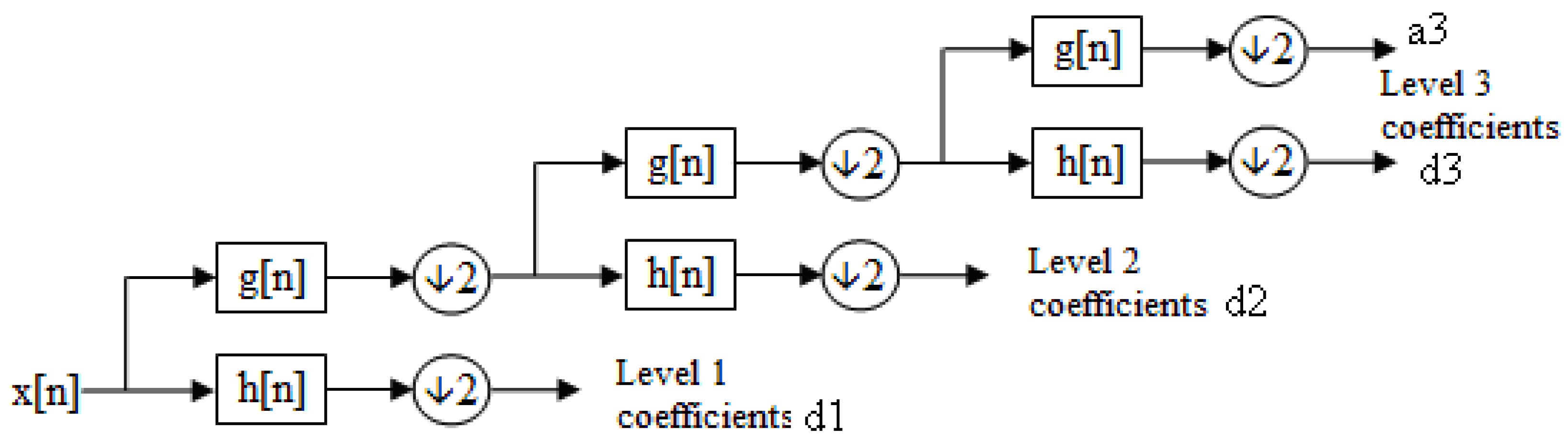
The wavelet transform represents signals using wavelets—localized basis functions that capture both time and frequency information, unlike the Fourier transform’s global sine and cosine functions. The discrete wavelet transform (DWT) decomposes a signal into scaled and translated versions of the mother wavelet, yielding approximation and detail coefficients [18,20]. Figure 10 illustrates this filter bank structure, with each level producing detail coefficients (d1)–(d3) from a high-pass filter and approximation coefficients (a3) from a low-pass filter at the final level.
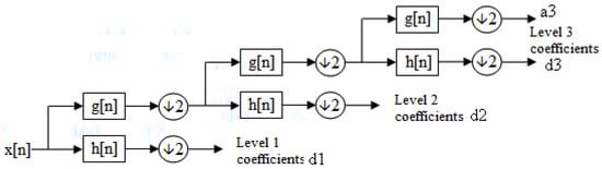
Figure 10.
Visualization of a filter bank structure used for extracting up to level-three coefficients by applying several high-pass (h[n]) and low-pass (g[n]) filters [21].
The Python package PyWavelets provides a robust library for wavelet transformations, with adjustable parameters and multiple forms of DWT [22]. The wavedec function enables multilevel DWT with a specified wavelet and decomposition level. For this analysis, the Daubechies 3 (db3) wavelet is used, known for its effectiveness in time series feature extraction and high-frequency noise reduction [23]. When set to None, the wavedec function calculates the maximum decomposition level as follows:
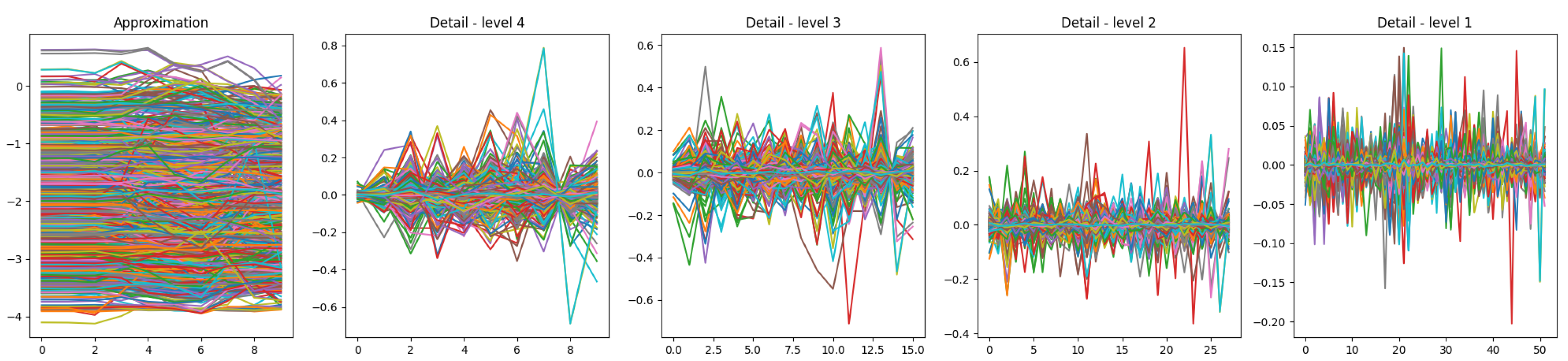
This ensures decomposition stops before the signal length falls below the wavelet’s . With a fixed of 100 and of 6 for db3, the maximum level here is 4. The function returns an array of coefficients, with approximation coefficients first, followed by detail coefficients from level n down to 1, as visualized in Figure 11 for the accelerometer x-axis.

Figure 11.
Visualization of the approximation coefficients as well as the detailed coefficients for the accelerometer x-axis.
4.2. Feature Selection
After extracting statistical, magnitude, FFT, and wavelet features, these are combined into a single feature set. However, not all features may be beneficial, particularly in combination. Hand-selecting features that complement each other, as discussed in Section 4.3, and calculating feature correlations, help determine which features to retain [24]. More features do not necessarily improve model performance, and irrelevant features may reduce it.
Feature correlation indicates relationships, i.e., a positive correlation means features A and B increase together, while a negative correlation means that as feature A increases, feature B decreases. Correlation values range from to 1, with 0 indicating no relationship. High correlations (near ±1) between features can cause multicollinearity, where one feature can be linearly predicted from another, potentially skewing results and compromising model accuracy.
4.2.1. Feature Correlation
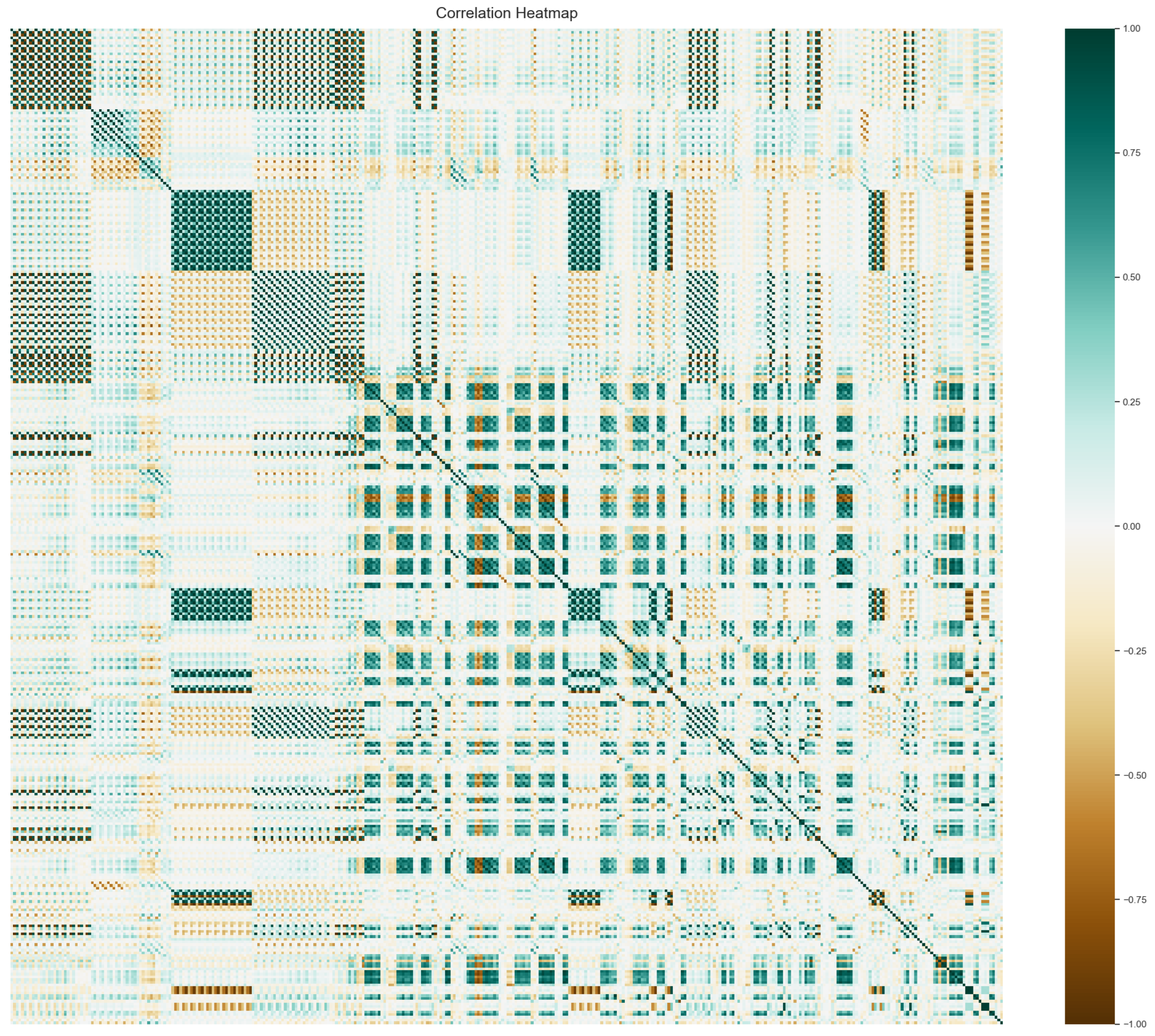
To address multicollinearity, highly correlated features can be removed from the feature set, which initially contained 370 features. The correlation matrix (Figure 12) visualizes these relationships.
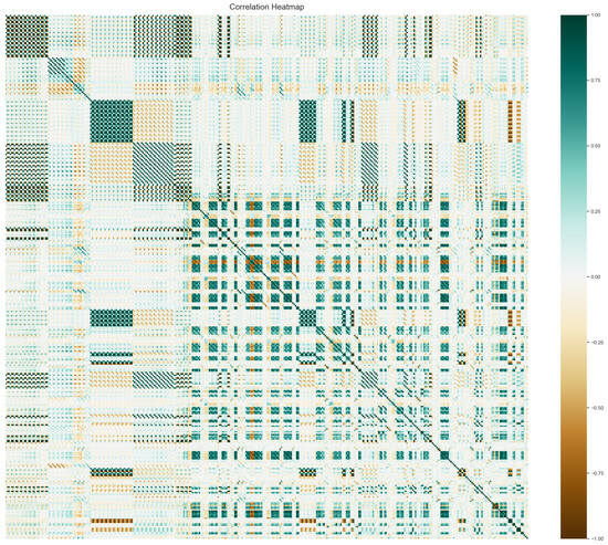
Figure 12.
Correlation matrix of all combined features (370).
A threshold is set to drop features above a certain correlation level. The Pearson method [25] calculates pairwise correlations, and for each feature, its average correlation with all others is computed. Features with higher average correlations are more redundant and are removed. For instance, if features A and B have a correlation exceeding the threshold, and feature A has a higher average correlation with other features, A is removed.
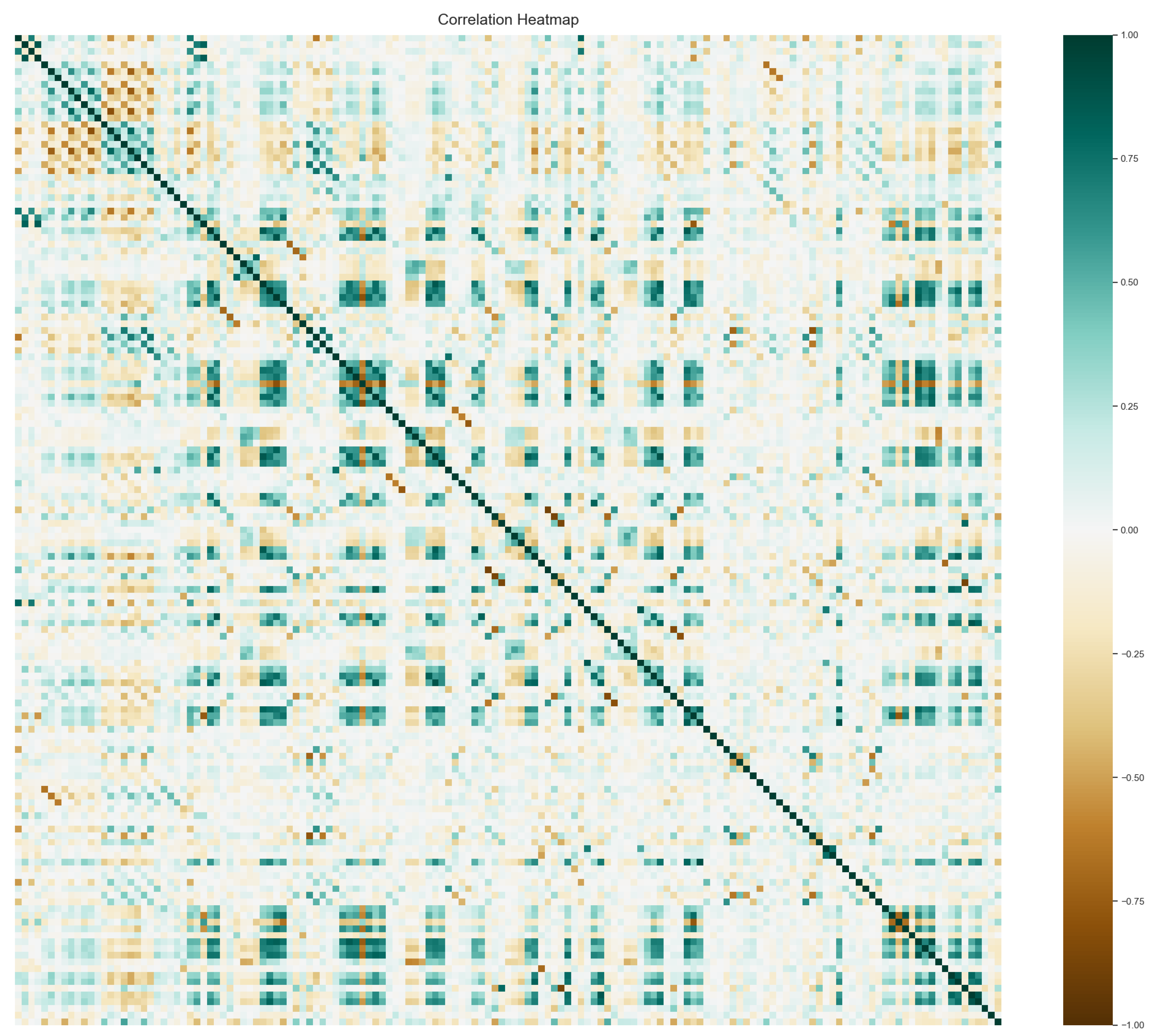
Using a threshold of 0.9, the feature set is reduced to 149 features. The resulting correlation matrix for this refined set is shown in Figure 13.
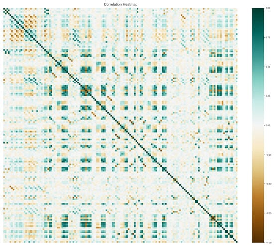
Figure 13.
Correlation matrix of all combined features, but features with a correlation between each other that is greater than 0.9 or lower than according to the Pearson correlation coefficient have been removed.
4.2.2. Principal Component Analysis
Principal component analysis (PCA) is a statistical technique used to reduce the dimensionality of a dataset while retaining as much variance as possible [26]. PCA transforms data into a new coordinate system, where each principal component (PC) represents a direction of maximum variance. PCs are ordered by variance, with the first PC capturing the most variance.
Dimensionality reduction is achieved by selecting a subset of PCs based on cumulative variance—often setting a threshold (e.g., 90% or 95%) depending on the data and goals. A high cumulative variance threshold includes fewer PCs if the last PCs contribute little to overall variance.
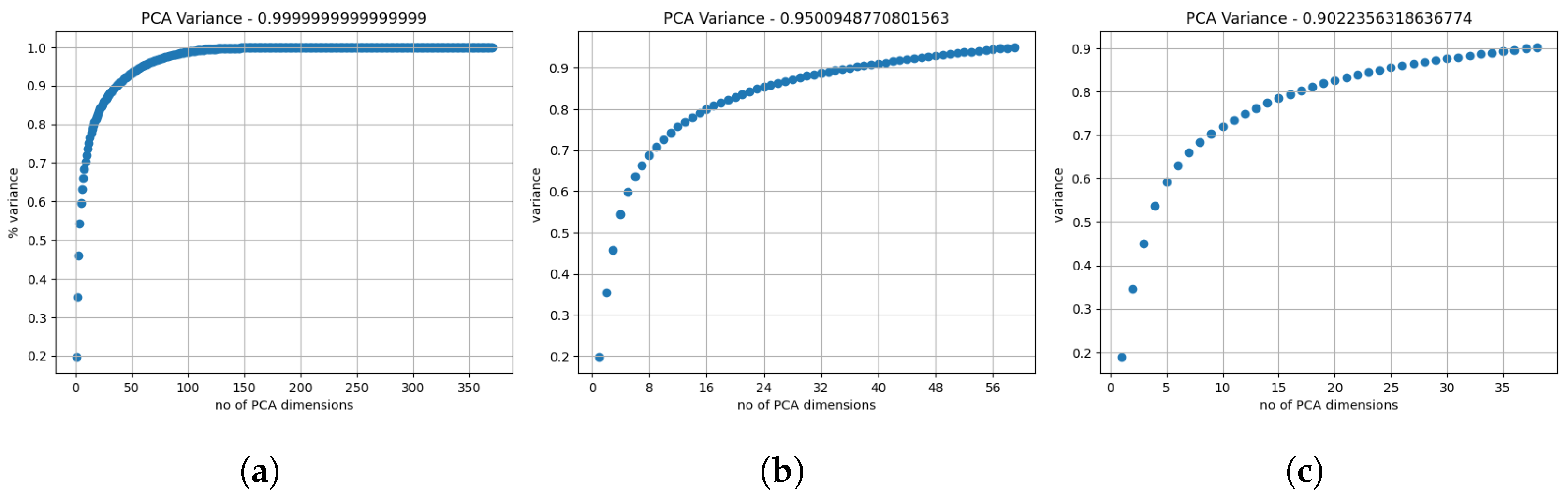
Applying PCA to our set of 370 features and plotting cumulative variance (Figure 14a) reveals that later PCs contribute minimally. Figure 14b,c show reduced sets achieving 0.95 and 0.9 cumulative variances with 59 and 38 PCs, respectively. By first reducing correlated features to 149 (see Section 4.2.1) and then applying PCA with a 0.9 variance threshold, we obtain a feature set of 37 PCs.
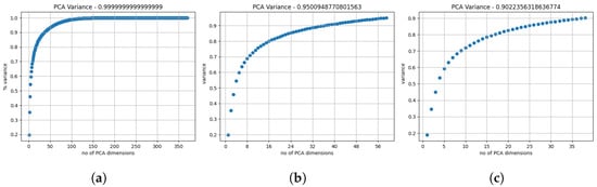
Figure 14.
Cumulative variance plotted in relation to the number of PCs used. (a) The total amount of PCs, accumulating in a variance of 1.0. (b,c) Using as many PCs as necessary to achieve a cumulative variance of 0.95 with 59 PCs and 0.9 with 38 PCs, respectively.
4.3. Constructing Feature Sets
After feature extraction and addressing multicollinearity with correlation analysis and PCA, the next step involves creating distinct feature sets. Different tasks may require specific features: statistical features might work well for some, while wavelet-based features or a combination using PCA could yield better results. To determine the optimal feature set, we constructed diverse sets by combining extracted features.
Note: For a better overview, the total number of feature sets is included at the end of each sentence in bold.
4.3.1. Raw and Combined Features
The raw time series serves as the baseline. Scaled and scaled + filtered versions of the raw data were used to create feature sets, with each sensor’s 3-axis data (accelerometer, gyroscope, magnetometer, and motion sensor) treated separately (4). Combined sets include IMU (accelerometer, gyroscope, magnetometer) and all sensors (6) for both scaled and scaled + filtered data (12).
For extracted features, each sensor was evaluated individually with each extraction technique (statistical, wavelet, frequency, magnitude). Combinations (e.g., accelerometer + gyroscope) were added, yielding 29 sets in total (41).
4.3.2. Feature Selection by Dimensionality Reduction
Beyond PCA and correlation-based reduction, additional sets were created using ANOVA F-test for the top features based on variance [27]. Using Python’s SelectKBest tool, 4 new sets were created with fractions of the original 370 features (185, 92, 61, 46) (45).
Additional sets were created by combining sensors (accelerometer + gyroscope, IMU, all sensors) and applying each feature extraction method, with correlated features removed at thresholds of 0.8 and 0.9, yielding 13 sets per threshold (71).
Finally, PCA was applied with cumulative variance thresholds of 0.95 and 0.9, with a combined approach of correlation removal and PCA at 0.9 (74).
In summary:
- Raw time series were scaled and filtered.
- Feature extraction methods (statistical, magnitude, FFT, wavelets) were applied.
- Dimensionality was reduced using PCA, correlation removal, and ANOVA F-test.
- Various feature combinations were created to evaluate sensor and feature effectiveness for smartphone posture recognition.
- A total of 74 feature sets were constructed.
5. Model Selection and Hyperparameter Tuning
After extracting several different features and building a multitude of feature sets, proper models have to be selected. Most predictive modeling techniques have adjustable parameters that allow the model to adapt to the underlying structure in the data [12]. Therefore, it is crucial to use the available data or rather the extracted features to determine the optimal values for these parameters, a process known as hyperparameter tuning. One common approach to model tuning involves dividing the available data into a training and a test set. While the training set is utilized to develop and fine-tune the model, the test set is used to estimate the model’s predictive performance.
The model selection and the tuning of their hyperparameters is a critical step in developing ML models and finally finding the best-suited model for a specific problem statement. But the hyperparameter tuning does not solely relate to the parameters of the ML models, but also to the training setup.
To achieve the goal of predicting the holding posture of the smartphone based on the extracted features mentioned and explained in Section 4, three popular machine learning models were utilized: SVM, random forest (RF), and k-nearest neighbors (KNN). We intentionally selected simpler models, as prior research (see Section 2) demonstrates their effectiveness within this domain. Moreover, existing studies indicate that these models perform robustly even with limited training data and are well-suited for direct execution on smartphones, which often have constrained computational resources.
5.1. Adjusting Number of Holding Postures
In the previous chapters, various feature sets have been built and comprehensive hyperparameter tuning for multiple ML models through grid search has been done to find the best-suited model and properly analyze the performance. However, during this process, two new approaches came up that could potentially further improve the results.
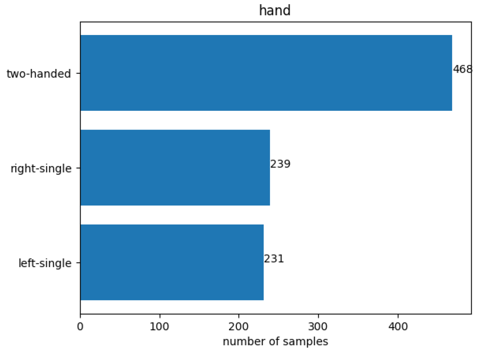
Firstly, the holding posture target variable was revisited and reevaluated whether those four postures shown in Figure 2 make the most sense. The most prominent use case for holding posture recognition for smartphones is to adjust the UI based on the holding hand. Taking this into consideration, an initial assumption is that the UI does not need to change drastically during both cradled postures. It should not make a big difference whether the right or the left hand holds the smartphone while the other hand is interacting with the touchscreen. Therefore, it might make more sense to combine the two cradled postures into one “two-handed” posture, to reduce the total number of holding postures (=target variable) from four down to three, which might further increase the detection performance by simplifying the classification task. By doing so, the number of samples per holding posture is now unevenly spread, as shown in Figure 15, as the posture two-handed contains samples from the previous postures right-double and left-double. If this distribution negatively affects the model’s performance, which can be observed through the confusion matrix, it may be necessary to address the issue by either removing certain samples from the two-handed group or augmenting samples from the other two postures. This approach aims to balance the distribution and improve the overall performance of the model, if necessary.

Figure 15.
Distribution of total samples per holding posture after combining the left-double and right-double postures into a single two-handed holding posture.
To evaluate the assumption that adjusting the number of holding postures increases the model’s performance, the same number of feature sets, as well as the models mentioned above, are tested for three holding postures.
5.2. Adjusting Length of Time Series
Additionally, during the data visualization conducted in Section 3, the idea came up to reduce the length of each time series from 1 s (0.5 s before and after each tap gesture) down to 0.8 or even 0.6 s (0.4 or 0.3 s before and after each gesture respectively). In Figure 5, it can be seen that the most important information lies in the middle of the time series, as this is the point in time where the touchscreen interaction happens. But the first and last 10% or maybe 20% (that is, 0.1 or 0.2 s, respectively) do not always contain valuable information. By discarding 20% or 40% of the total time series, the feature extraction process is less computationally expensive and the model might perform better with those smaller time series with higher information density.
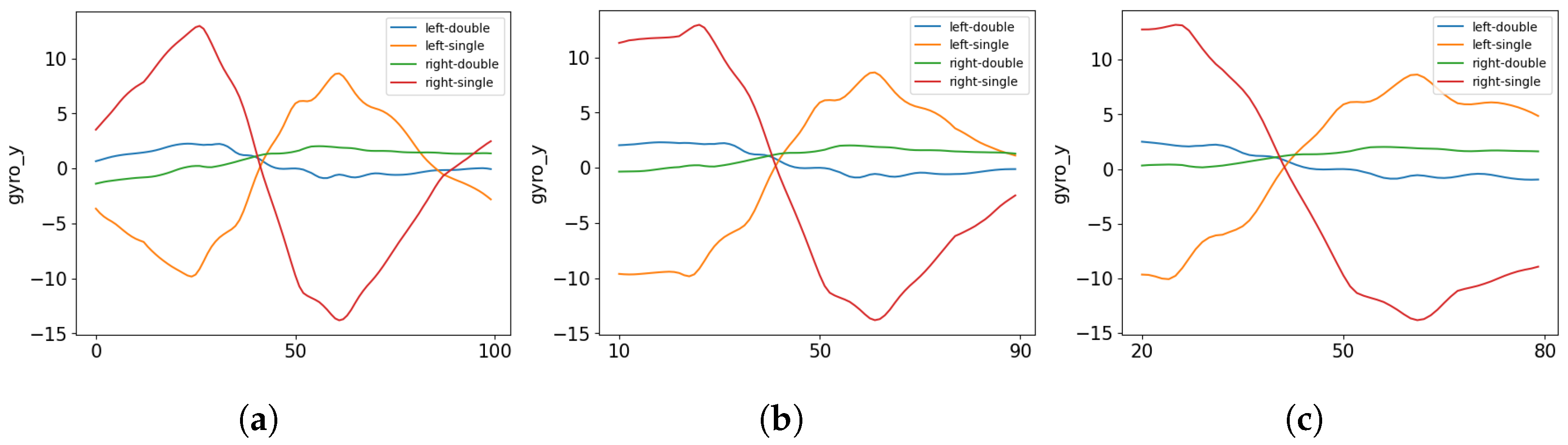
This approach is implemented and visualized in Figure 16 with the gyroscope Y-axis. The data are grouped by the holding posture, and the average over all samples is computed. To facilitate the comparison, the initial and final 0.1 and 0.2 s of the time series are removed. Upon inspection, it is observed that most of the information remains even with the removal of 0.1 s. However, the 0.2-s cut may result in a significant loss of information. Therefore, as a starting point, the entire pipeline is trained using a 0.1-s cut, resulting in a time series containing 0.8 s of data.
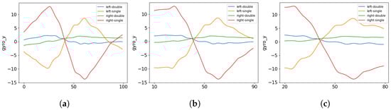
Figure 16.
Comparison of sensor data from a single axis (gyroscope Y-axis) at a specific location (middle of the touchscreen), grouped by holding posture and averaged across all samples. It includes (a) the raw data, (b) data trimmed by 0.1 s on both ends, and (c) data trimmed by 0.2 s on both ends to shorten the time series.
6. Results and Evaluation
In the preceding sections, diverse feature sets were constructed, and an extensive hyperparameter grid search for various ML models was performed. All models were trained using 5-fold cross-validation (CV), totaling 297,840 models. Now, with a multitude of models at hand, the next objective is to evaluate their performances using different metrics. This evaluation process aims to identify the optimal model that exhibits the best overall performance for this classification task. Several factors need to be taken into account, such as the feature set used (because of the computational effort required for the model), the number of features, and various performance metrics (for example, CV scores, Kappa statistic, confusion matrices, the receiver operating characteristic (ROC), and the area under the curve (AUC)). Because of the number of different models as well as evaluation metrics, it is necessary to apply smart filtering and focus on the analysis of the most promising models afterward.
6.1. Raw Time-Series Data
An initial look at all models shows that the KNN model never outperformed the other models and was often far behind in performance. The overall median CV score across all KNN models was 0.7971, while the SVM and RF achieved 0.8602 and 0.8708, respectively. Depending on the feature sets used, the SVM sometimes outperformed the RF. Furthermore, data augmentation significantly improved the performance of the models. This improvement may be due to the small initial dataset of only 723 samples and suggests that a larger, more diverse dataset would greatly benefit this ML task.
Despite the absence of any feature preprocessing—besides normalization of the data—the RF achieved a surprising 87.9% CV score using only the IMU data and an 87.2% CV score with the same feature set but after applying a rolling median filter, effectively reducing the number of features from 902 to 92. The latter model serves as a baseline and successfully demonstrates that the holding posture can be extracted from the data. As the models in Section 6.2 will be assessed using additional performance metrics, the baseline model reached the following values:
- CV score: 0.872.
- ACC on test set: 0.899.
- kappa: 0.865.
- AUC: 0.984.
6.2. First Selection of the Most Valuable Models
The feature extraction methods aim to further reduce the complexity of the model by decreasing the number of features necessary while still obtaining a high accuracy (ACC) score.
6.2.1. Four Postures, Combined Features
After the first observation of the overall performances of the three different ML models, as well as an analysis of the raw time series as a feature set, the next step is to evaluate the models that utilized extracted features. In this initial model selection, the metrics CV, test set ACC, Kappa, and AUC are evaluated. To focus on the top-performing models, Table 2 displays only those models that surpassed the 95th percentile in at least one performance metric.
Table 2.
First model selection of the Comb. Features iteration that contained different feature set variations of the extracted features. The iteration consisted of 29 feature sets, and only those model + feature set combinations are shown that surpassed the 95th percentile in at least one performance metric. Bold row = overall best-performing model.
When examining the models in Table 2, the AUC values are quite similar, ranging from 0.984 to 0.994, while other metrics show more diversity, such as the CV score, which ranges from 0.894 to 0.93. The accuracies on the test set are also quite close together, which makes it hard to pick one model over the other. One possible solution is to examine the number of features and which features are used. For example. For example, the SVM—Comb. Features model utilized all 370 features, meaning that every single feature extraction method needed to be implemented, but it achieved lower CV, Kappa, and ACC scores on the test set compared to the RF—Wavelets Gyro model, which only used 32 features in total and only a wavelet transform, making it far less complex. Considering the complexity of the model by the number and type of features used, the preferred model in this iteration is RF—Wavelets IMU as it achieved the best overall CV score (93%), the best Kappa score (90.5%), and the best AUC score (99.4%).
6.2.2. Four Postures, Combined Features with Dimensionality Reduction
Table 3 lists all models that surpassed the 95th percentile in any performance metric while implementing at least one form of dimensionality reduction. This can be verified by examining the number of features in the feature sets. For example, the Wavelets IMU feature set contains 92 features in Table 2 and only 32 and 27 features in Table 3, using 0.9 and 0.8 correlation filters, respectively.
Table 3.
Model selection of all feature sets that contained extracted features and used some form of dimensionality reduction, such as PCA, correlation filtering, or SelectKBest features. Only those model + feature set combinations are shown that surpassed the 95th percentile in at least one performance metric. “corr.” in the feature set refers to “correlation”, which means a correlation filter is implemented with a certain threshold. Bold row = overall best-performing model.
First, it can be observed that the range between the best and worst model for each performance metric widened significantly with the application of dimensionality reduction. This may be due to the excessive loss of information as a trade-off for reducing the number of features. In terms of numerical results, the SVM—SelectKBest model with 61 features performed the worst, with a CV score of 0.85. On the other hand, the best performance of 0.93 was achieved by the RF—Wavelets IMU (0.9 corr.) model, which means there is a spread of 7% in the CV score.
6.2.3. Three Postures, Combined Features with Dimensionality Reduction
The dimensionality reduction did not worsen any performance metric, in fact, some even improved with fewer features. For this reason, only those feature sets will be analyzed for the next iterations, starting with the analysis of the reduction of holding postures from four down to three, as seen in Table 4.
Table 4.
Apart from reducing the holding postures from 4 down to 3, the overall structure remains the same as in Table 3. Bold row = overall best-performing models.
The first observation in this iteration is that far more SVM models (12) are in the 95th percentile compared to RF models (4), which contrasts with the results from the same feature sets with four holding postures. Differentiating between right-double and left-double might be challenging for the large-margin classifier, as it is difficult to visually distinguish these two target variables from the sensor data plots shown in Section 3. Therefore, the SVMs performed better overall with three holding postures rather than four.
Overall, all models performed comparably to those trained on the dataset with four holding postures. There was no significant improvement in performance. Using the dataset with three holding postures comes at the cost of class imbalance, as the two-handed class has about double the number of samples than the other classes. Therefore, the Kappa metric should be more suitable than the test set ACC for this iteration. In that case, the highest score of 93.9% was achieved by SVM—Comb. Features (0.8 corr.) and is nearly 1.5% lower than the best-performing model utilizing all four holding postures. Moreover, only the AUC values of those two models are pretty similar, while for the other metrics, the RF with four classes outperformed the SVM with three postures, especially when looking at the complexity. The SVM used 111 features from the combined extracted features, which means that all four feature extraction methods needed to be calculated, on the other hand, the RF only used 32 wavelet features.
The top performing model for any PCA feature set was exclusively the SVM, with the best model being the SVM—PCA 0.95 var. (0.9 corr.). When comparing it to the SVM—Comb. Features (0.8 corr.), there is no clear winner, as some performance metrics favor one model while others favor the other. In terms of complexity, both models use all combined features and apply a correlation filter, and one model implements PCA on top of the correlated features, further decreasing the number of features from 111 down to 60.
However, despite the limited information gained from distinguishing between four holding postures instead of three for dynamic UI design adjustments, none of the models with only three classes performed significantly better than the top model with four postures. This clearly favors the best model with four target variables, as it captures a greater amount of overall information.
6.2.4. Combined Features with Dimensionality Reduction and a 100 ms Cutoff
Cutting off some parts of each time series in order to reduce the length aims to increase or at least sustain the current model accuracies. This approach is tested with four holding postures as well as with the class-imbalanced dataset with only three postures. Not all feature sets were tested, only those that implemented at least one form of dimensionality reduction, namely PCA, correlation filtering, or the SelectKBest algorithm. Table 5 shows the differences between both datasets. Only SVM and RF models were used for the median calculation, as those were the best-performing models and KNNs might distort the median value. Surprisingly, the three-posture models performed significantly better across all metrics when using shorter time series (in this case, a 100 ms cutoff at each end of the time series).
Table 5.
Comparison of the median values for each performance metric across all feature sets that include any form of dimensionality reduction (PCA, correlation filter, SelectKBest) between three and four holding postures, using a 100 ms cutoff in each time series.
Therefore, only the best models using three postures that exceeded the 95th percentile in at least one metric are shown in Table 6. Again, because of class imbalance, the ACC and, therefore, the CV score should not be taken too seriously without taking into account the Kappa value. Only looking at the CV score as well as the ACC on the test set, all models seem to perform exceptionally well, often reaching accuracies of over 95%. The Kappa values are very comparable to those in Table 4, suggesting that the overall models did not improve prediction performance for all target variables.
Table 6.
Same structure and setup as explained in Table 4 but with a 100 ms cutoff on each end of each time series. Bold row = overall best-performing model.
Nevertheless, this test effectively demonstrated that using a time series of 1 s is not required, and a shorter time frame proves to be adequate. The best overall model in this iteration is the “RF—Wavelets all (0.9 corr.)” model, which bears similarity to the top models from the iteration involving three holding postures but a 1-s time series. However, in this case, the feature set consisted only of 28 wavelet features instead of the combined 111 or 60 previously used.
6.3. Detailed Analysis
After all these training iterations and evaluations, which yielded a multitude of different models with different training setups, such as for three or four holding postures, the next step is to analyze those models in more detail. Important metrics for analyzing the performance of each model for each target variable include confusion matrices and ROC curves for each class. The following models were selected after the initial screening in Section 6.2, and appear to be the most interesting ones:
- RF—IMU raw scaled + filtered—four postures.
- RF—Wavelets IMU—four postures.
- RF—Wavelets all (0.9 corr.)—four postures.
- SVM—Comb. Features (0.8 corr.)—three postures.
- SVM—PCA 0.95 var. (0.9 corr.)—three postures.
- RF—Wavelets all (0.9 corr.)—three postures (100 ms cutoff).
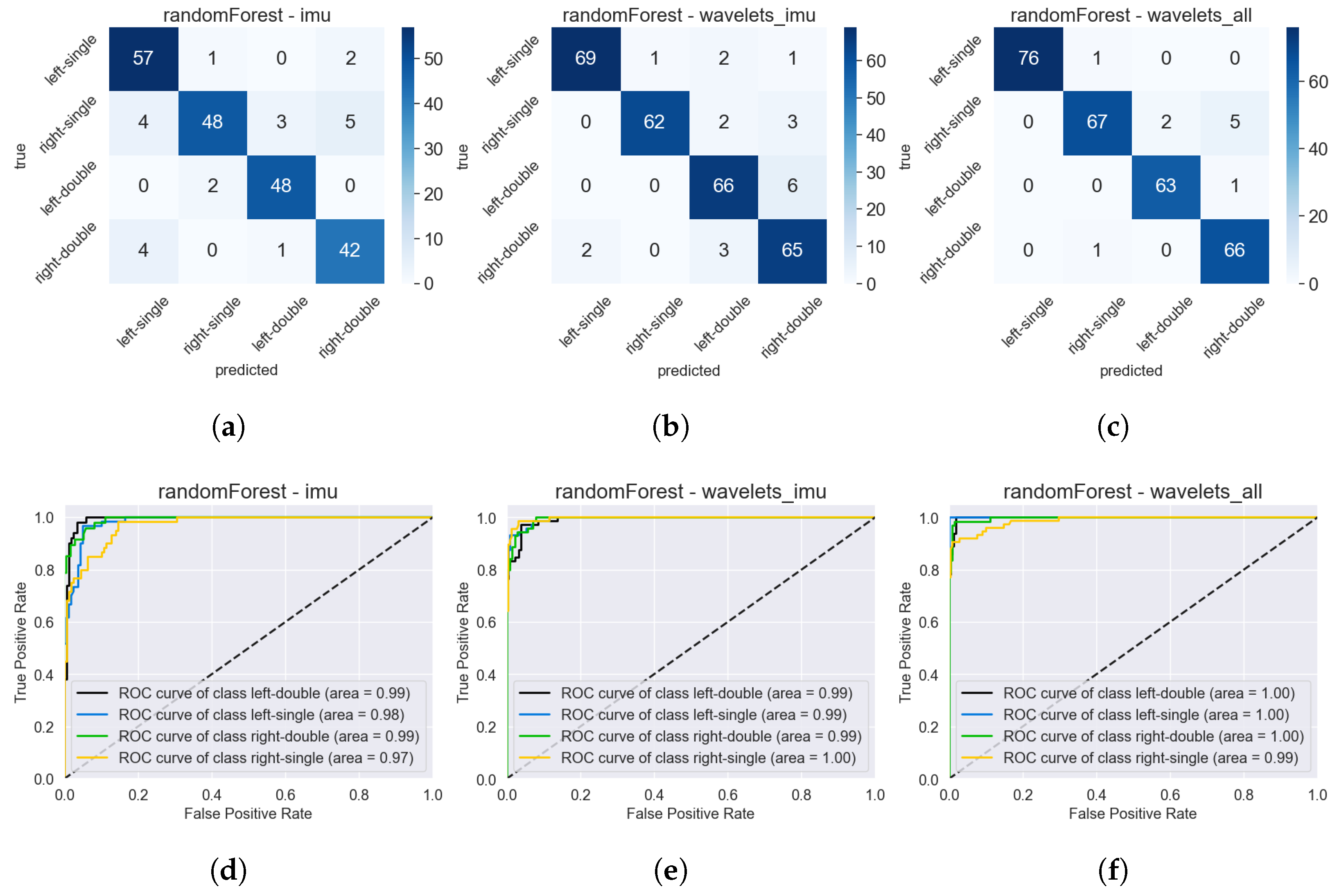
Surprisingly, in Figure 17d, the ROC curves of the baseline model for each class reveal that the right-single class performs the worst, despite all participants being right-handed. From the first estimation, the left-single class was expected to have poorer performance, as it is less natural for participants to operate their phone with the left hand, likely resulting in shakier sensor data and making this class more challenging to predict. This phenomenon is not present in the other models (Figure 17e,f), where all classes achieved an individual AUC score of either 0.99 or even 1.00. From the individual ROC curves alone, a superior model cannot be determined between Figure 17e,f.

Figure 17.
Confusion matrix and ROC curves for three different models: The baseline model with raw time series scaled and filtered (a,d), the RF with wavelet features from the IMU (b,e), and the RF with all wavelet features and a 0.9 correlation filter (c,f). All models used the dataset with four holding postures.
In the confusion matrices shown in Figure 17, it is clear that both models (Figure 17b,c) make fewer overall prediction errors, despite utilizing a 30% augmented dataset and, hence, a larger sample size. Although neither model demonstrated significantly superior performance based on the confusion matrix, the model RF—Wavelets all with a 0.9 correlation filter (Figure 17c,f) is preferable as it implements a dimensionality reduction and only uses 32 features.
The final model for predicting four holding postures is as follows:
- Model: RF with max_depth = 60, max_features = 2, n_estimators = 1000.
- Feature set: wavelets all with 0.9 correlation filter, 32 features in total.
- CV score: 93.0%.
- ACC on test set: 96.5%.
- Kappa: 95.3%.
- AUC: 0.995.
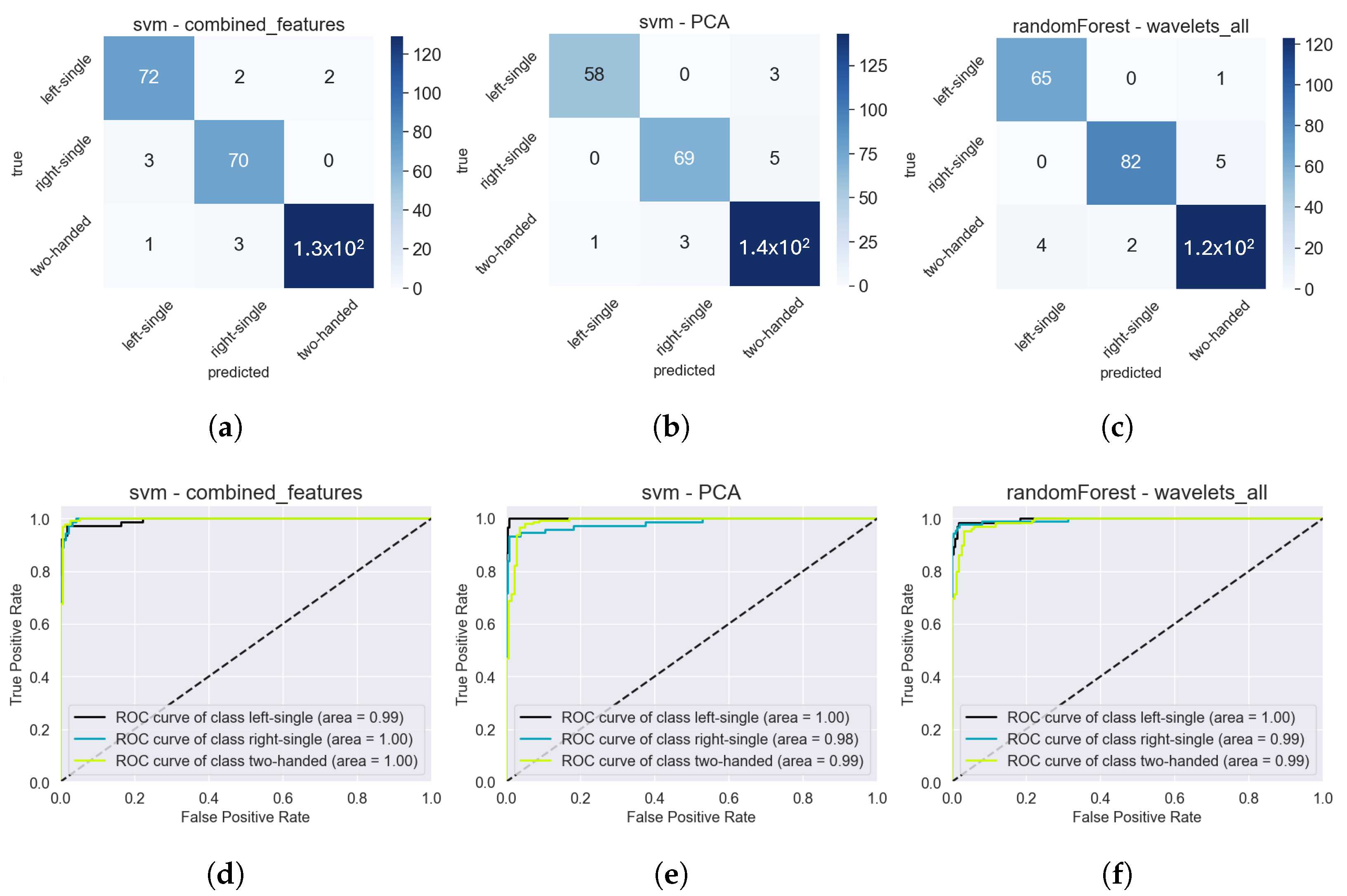
When analyzing the best model for three holding postures, all three models shown in Figure 18 used the same 30% augmented dataset, resulting in an equal number of samples. Only the train-test split affects the distribution of the target variables. Considering that there are about twice as many samples for the two-handed class, it is impressive that the number of incorrect predictions is not proportionally higher than those for the other two classes. In fact, the first model, Figure 18a, even predicted the left-single class wrong twice as often as the two-handed class.
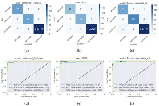
Figure 18.
Confusion matrix and ROC curves for three different models: The SVM with combined features and a 0.8 correlation filter (a,d), the SVM with PCA features and a 0.9 correlation filter (b,e), and the RF with all wavelet features, a 0.9 correlation filter, and a 100 ms cutoff (c,f). All models used the dataset with three holding postures.
All three ROC curves for each class are very similar in shape as well as AUC score. Therefore, the only relevant factor differentiating them is complexity. Both SVMs used the combined feature set and, therefore, all feature extraction methods. The second SVM applied a PCA transform, resulting in a total of 60 features, while the other SVM used 111 features. This is the only major difference compared to the third model, an RF with all wavelet features, a correlation filter of 0.9, and a 100 ms cutoff at both ends of each time series. This model required only 28 wavelet features and is, therefore, preferred overall due to its lower complexity.
These are the detailed characteristics of the final model used for predicting three holding postures:
- Model: RF with max_depth = 20, max_features = 4, n_estimators = 3000.
- Feature set: dataset with 0.8 s time series, wavelets all with a 0.9 correlation filter, 28 features in total.
- CV score: 94.7%.
- ACC on test set: 95.7%.
- Kappa: 93.4%.
- AUC: 0.993.
7. Conclusions
7.1. Summary
By analyzing the sensor data of the built-in IMU of smartphones it was possible to detect the holding posture during the usage of an app with an accuracy of 95.7% without the need for external sensors. Therefore, the model is hardware- and platform-independent and can be shipped on Android and iOS applications. With the knowledge of the holding posture of the user at runtime, the UI designer can consider this information while designing an intuitive interface. Also, self-adaptive capabilities in terms of the UI of a smartphone could be imaginable with real-time recognition of holding postures. Furthermore, gesture-based interactions can be implemented based on posture, such as taking screenshots while holding the phone in one hand using a combination of a long press and sliding motion.
Various data preprocessing and feature extraction methods have been applied, including statistical features of the raw time series, FFT, wavelet transform, and magnitude features. After normalizing the features, a total of 74 different feature sets were constructed to analyze different sensors, axes, and feature extraction methods.
Next up, a thorough hyperparameter tuning was conducted for KNN, SVM, and RF. Each of the 272 different models was trained with every feature set and validated using 5-fold cross-validation, resulting in a total of 99,280 model fits. During the feature extraction process, two new approaches emerged that could potentially increase model accuracy and reduce complexity. The first approach involved reducing the number of holding postures from four down to three by combining the two two-handed postures, right-double and left-double, into one two-handed posture. This idea primarily arose after analyzing the raw sensor data, which showed that the two two-handed gestures shared very similar sensor behaviors. Furthermore, the question arose of whether a 1-s time series is overkill. Therefore, 0.1 s was trimmed from each end of the time series, effectively reducing the duration to 0.8 s. Both approaches were tested with each ML model from hyperparameter tuning as well as with every feature set, bringing the total number of training fits to 297,840.
Finally, to evaluate all these models and find the best-suited one for this problem statement, multiple performance metrics were used, including the CV score, accuracy on the test set, Kappa, and AUC value. To evaluate the effectiveness of the feature extraction methods, the raw time series were used as feature sets, serving as baselines for comparisons. The best model that used raw data achieved an 87.9% CV score. Interestingly, the raw time series data performed way better than initially expected; however, feature engineering increased the overall accuracy and reduced the complexity of the model.
After analyzing multiple models, two final models were chosen based on the individual ROC curves for each class, the confusion matrix, as well as the complexity. One model was chosen for predicting four holding postures, and the other one was only able to predict three postures. Because of the class imbalance, it makes more sense to compare these two models by the Kappa value rather than the test set accuracy. Even though the accuracy of the model predicting four holding postures exceeds that of the model with three holding postures, the Kappa value and, to a lesser extent, the AUC value are also higher. Hence, the single most preferable model overall is the RF predicting four different holding postures, achieving an accuracy of 95.7% on the test set.
When comparing this model to the baseline model, which only used the raw time series data, it can be concluded that all performance metrics improved with proper data preprocessing, feature extraction, and dimensionality reduction. Notably, the CV score, accuracy on the test set, and Kappa value increased significantly, while the model’s complexity was reduced due to the use of fewer features. Nevertheless, the raw time series data already achieved very high performance metrics without any data preprocessing, suggesting that the data recording setup and the sensor data used are well-suited for this task.
The implications of this model extend beyond the current functionality, offering a foundation for dynamic user interface adjustments that can accommodate various user needs and preferences in real-time. By enabling smartphones to detect posture shifts, this model supports adaptive UIs that could reduce user fatigue, improve accessibility for individuals with different physical abilities, and provide context-aware features for safer mobile interactions. These findings invite further exploration into posture recognition across other mobile devices and environments, broadening the potential impact of this work on future smartphone designs and user-centric technology.
7.2. Future Work
The current sample size is relatively limited, comprising data from nine volunteers. Although we supplemented this dataset with a 30% increase through data augmentation, the initial participant group was deliberately chosen to reflect a range of smartphone proficiency levels. This strategy introduces some diversity in user experience; however, it does not fully capture the range of potential user demographics. To enhance the representativeness and robustness of our findings, future studies will expand the dataset to include a larger and more varied participant pool, targeting diverse user groups. This planned extension will enable more generalizable insights and strengthen the study’s overall validity.
Currently, this model is limited to recognizing tap gestures; however, future developments will aim to incorporate support for swipe gestures using a dynamic time-warping (DTW) approach. Expanding the dataset with additional recordings will not only enhance the model’s generalizability but will also be essential for exploring neural network architectures, which require a significantly larger volume of data. Furthermore, future work will consider the integration of advanced time-series classification models, such as HIVE-COTE [28], InceptionTime [29], and transformer-based architectures [30], which are recognized for their effectiveness in handling complex time-series data.
Furthermore, participants were instructed to interact with a 3 × 3 grid on the touchscreen, focusing on key areas commonly used in smartphone applications. While recognition within these predefined regions performs well, collecting additional data from interactions outside the grid, as well as incorporating various smartphone sizes, may enhance accuracy and generalizability across diverse usage scenarios.
Author Contributions
Conceptualization, R.H. and M.K.; methodology, R.H.; software, R.H.; validation, R.H., M.K. and E.S.; formal analysis, R.H.; investigation, R.H.; resources, R.H.; data curation, R.H.; writing—original draft preparation, R.H.; writing—review and editing, R.H., M.K. and E.S.; visualization, R.H.; supervision, M.K.; project administration, M.K.; funding acquisition, M.K. All authors have read and agreed to the published version of the manuscript.
Funding
This research received no external funding.
Data Availability Statement
The data presented in this study are available on request from the corresponding author due to legal reasons.
Conflicts of Interest
Author Rene Hörschinger was employed by the company Windpuls GmbH. The remaining authors declare that the research was conducted in the absence of any commercial or financial relationships that could be construed as a potential conflict of interest.
Abbreviations
The following abbreviations are used in this manuscript:
| ACC | accuracy |
| AUC | area under the curve |
| CV | cross-validation |
| DTW | dynamic time warping |
| DWT | discrete wavelet transform |
| FFT | fast Fourier transform |
| IMU | inertial measurement unit |
| KNN | k-nearest neighbors |
| ML | machine learning |
| PC | principal component |
| PCA | principal component analysis |
| RF | random forest |
| ROC | receiver operating characteristic |
| SVM | support vector machine |
| UI | user interface |
References
- Hoober, S. How Do Users Really Hold Mobile Devices? UX Matters, 18 February 2013. [Google Scholar]
- Hardyck, C.; Petrinovich, L.F. Left-handedness. Psychol. Bull. 1977, 84, 385. [Google Scholar] [CrossRef] [PubMed]
- Wimmer, R.; Boring, S. HandSense: Discriminating different ways of grasping and holding a tangible user interface. In Proceedings of the 3rd International Conference on Tangible and Embedded Interaction, Cambridge, UK, 16–18 February 2009; pp. 359–362. [Google Scholar]
- Löchtefeld, M.; Schardt, P.; Krüger, A.; Boring, S. Detecting users handedness for ergonomic adaptation of mobile user interfaces. In Proceedings of the 14th International Conference on Mobile and Ubiquitous Multimedia, Linz, Austria, 30 November–2 December 2015; pp. 245–249. [Google Scholar]
- Avery, J.; Vogel, D.; Lank, E.; Masson, D.; Rateau, H. Holding patterns: Detecting handedness with a moving smartphone at pickup. In Proceedings of the IHM ’19: 31st Conference on l’Interaction Homme-Machine, Grenoble, France, 10–13 December 2019; Association for Computing Machinery: New York, NY, USA, 2019; pp. 1–7. [Google Scholar] [CrossRef]
- Goel, M.; Wobbrock, J.; Patel, S. GripSense: Using built-in sensors to detect hand posture and pressure on commodity mobile phones. In Proceedings of the UIST ’12: 25th Annual ACM Symposium on User Interface Software and Technology, Cambridge, MA, USA, 7–10 October 2012; Association for Computing Machinery: New York, NY, USA, 2012; pp. 545–554. [Google Scholar] [CrossRef]
- Goel, M.; Jansen, A.; Mandel, T.; Patel, S.N.; Wobbrock, J.O. ContextType: Using hand posture information to improve mobile touch screen text entry. In Proceedings of the SIGCHI Conference on Human Factors in Computing Systems, Paris, France, 27 April–2 May 2013; pp. 2795–2798. [Google Scholar]
- Park, C.; Ogawa, T. A Study on Grasp Recognition Independent of Users’ Situations Using Built-in Sensors of Smartphones. In Proceedings of the Adjunct Proceedings of the 28th Annual ACM Symposium on User Interface Software & Technology, Daegu, Republic of Korea, 8–11 November 2015; pp. 69–70. [Google Scholar]
- Hoober, S. Design for Fingers, Touch, and People, Part 1. UX Matters, 6 March 2017. [Google Scholar]
- Géron, A. Hands-On Machine Learning with Scikit-Learn and TensorFlow: Concepts, Tools, and Techniques to Build Intelligent Systems; O’Reilly Media: Sebastopol, CA, USA, 2017. [Google Scholar]
- Dunford, R.; Su, Q.; Tamang, E. The pareto principle. Plymouth Stud. Sci. 2014, 7, 140–148. [Google Scholar]
- Kuhn, M.; Johnson, K. Applied Predictive Modeling; Springer: New York, NY, USA, 2013; Volume 26. [Google Scholar]
- Sv, M. Calculate Skewness in Python (with Examples), July 2021. Available online: https://towardsdatascience.com/calculate-skewness-in-python-with-examples-pyshark-b7467dfa166d (accessed on 10 October 2024).
- Sv, M. Calculate Kurtosis in Python (with Examples), September 2021. Available online: https://towardsdatascience.com/calculate-kurtosis-in-python-with-examples-pyshark-2b960301393 (accessed on 10 October 2024).
- Brownlee, J. Gentle Introduction to Vector Norms in Machine Learning. 2021. Available online: https://machinelearningmastery.com/vector-norms-machine-learning/ (accessed on 14 November 2024).
- Bryan, P.B. Fourier Transform, Applied (1): Introduction to the Frequency Domain. 2021. Available online: https://towardsdatascience.com/the-fourier-transform-1-ca31adbfb9ef (accessed on 14 November 2024).
- Bryan, P.B. Fourier Transform, Applied (2): Understanding Phase Angle. 2021. Available online: https://towardsdatascience.com/the-fourier-transform-2-understanding-phase-angle-a85ad40a194e (accessed on 14 November 2024).
- Alegeh, N.; Thottoli, M.; Mian, N.; Longstaff, A.; Fletcher, S. Feature Extraction of Time-Series Data Using DWT and FFT for Ballscrew Condition Monitoring. In Advances in Manufacturing Technology XXXIV: Proceedings of the 18th International Conference on Manufacturing Research, Incorporating the 35th National Conference on Manufacturing Research, Derby, UK, 7–10 September 2021; IOS Press: Amsterdam, The Netherlands, 2021; Volume 15, p. 402. [Google Scholar]
- Kutz, J.N. Data-Driven Modeling & Scientific Computation: Methods for Complex Systems & Big Data; Oxford University Press: Oxford, UK, 2013. [Google Scholar]
- Olkkonen, J.T. Discrete Wavelet Transforms; IntechOpen: Rijeka, Croatia, 2011. [Google Scholar] [CrossRef]
- Hanif, M.; Dwivedi, U.; Basu, M.; Gaughan, K. Wavelet based islanding detection of DC-AC inverter interfaced DG systems. In Proceedings of the 45th International Universities Power Engineering Conference UPEC2010, Cardiff, UK, 31 August–3 September 2010; pp. 1–5. [Google Scholar]
- Lee, G.R.; Gommers, R.; Waselewski, F.; Wohlfahrt, K.; O’Leary, A. PyWavelets: A Python package for wavelet analysis. J. Open Source Softw. 2019, 4, 1237. [Google Scholar] [CrossRef]
- Arya, S.J.; Jisha, V.R.; Ponmalar, M.; Usha, K.; Haridas, T.R. Implementation and Performance Assessment of Wavelet Prefiltered Platform Tilt Computation Using Low-cost MEMS IMU. In Proceedings of the 2022 IEEE 1st International Conference on Data, Decision and Systems (ICDDS), Bangalore, India, 2–3 December 2022; pp. 1–6. [Google Scholar] [CrossRef]
- Katrutsa, A.; Strijov, V. Comprehensive study of feature selection methods to solve multicollinearity problem according to evaluation criteria. Expert Syst. Appl. 2017, 76, 1–11. [Google Scholar] [CrossRef]
- Sedgwick, P. Pearson’s correlation coefficient. BMJ 2012, 345. [Google Scholar] [CrossRef]
- Jolliffe, I. Principal Component Analysis; Springer: New York, NY, USA, 2002. [Google Scholar]
- Abouloifa, H.; Bahaj, M. Predicting late delivery in Supply chain 4. In 0 using feature selection: A machine learning model. In Proceedings of the 2022 5th International Conference on Advanced Communication Technologies and Networking (CommNet), Marrakech, Morocco, 12–14 December 2022; pp. 1–5. [Google Scholar] [CrossRef]
- Middlehurst, M.; Large, J.; Flynn, M.; Lines, J.; Bostrom, A.; Bagnall, A. HIVE-COTE 2.0: A new meta ensemble for time series classification. Mach. Learn. 2021, 110, 3211–3243. [Google Scholar] [CrossRef]
- Ismail Fawaz, H.; Lucas, B.; Forestier, G.; Pelletier, C.; Schmidt, D.F.; Weber, J.; Webb, G.I.; Idoumghar, L.; Muller, P.A.; Petitjean, F. Inceptiontime: Finding alexnet for time series classification. Data Min. Knowl. Discov. 2020, 34, 1936–1962. [Google Scholar] [CrossRef]
- Zerveas, G.; Jayaraman, S.; Patel, D.; Bhamidipaty, A.; Eickhoff, C. A transformer-based framework for multivariate time series representation learning. In Proceedings of the 27th ACM SIGKDD Conference on Knowledge Discovery & Data Mining, Singapore, 14–18 August 2021; pp. 2114–2124. [Google Scholar]


Disclaimer/Publisher’s Note: The statements, opinions and data contained in all publications are solely those of the individual author(s) and contributor(s) and not of MDPI and/or the editor(s). MDPI and/or the editor(s) disclaim responsibility for any injury to people or property resulting from any ideas, methods, instructions or products referred to in the content. |
© 2024 by the authors. Licensee MDPI, Basel, Switzerland. This article is an open access article distributed under the terms and conditions of the Creative Commons Attribution (CC BY) license (https://creativecommons.org/licenses/by/4.0/).