Neural Architecture Search via Trainless Pruning Algorithm: A Bayesian Evaluation of a Network with Multiple Indicators

Abstract

Neural Architecture Search (NAS) has found applications in various areas of computer vision, including image recognition and object detection. An increasing number of algorithms, such as ENAS (Efficient Neural Architecture Search via Parameter Sharing) and DARTS (Differentiable Architecture Search), have been applied to NAS. Nevertheless, the current Training-free NAS methods continue to exhibit unreliability and inefficiency. This paper introduces a training-free prune-based algorithm called TTNAS (True-Skill Training-Free Neural Architecture Search), which utilizes a Bayesian method (true-skill algorithm) to combine multiple indicators for evaluating neural networks across different datasets. The algorithm demonstrates highly competitive accuracy and efficiency compared to state-of-the-art approaches on various datasets. Specifically, it achieves 93.90% accuracy on CIFAR-10, 71.91% accuracy on CIFAR-100, and 44.96% accuracy on ImageNet 16-120, using 1466 GPU seconds in NAS-Bench-201. Additionally, the algorithm exhibits improved adaptation to other datasets and tasks.

1. Introduction

Convolutional Neural Networks (CNNs) have played a pivotal role in driving forward the field of computer vision, leading to notable advancements and breakthroughs. Despite their transformative impact, the design of architectures tailored to specific computer vision tasks continues to be a labor-intensive process that is heavily reliant on human expertise. Despite the paradigm shift from traditional feature engineering to architecture design, the process remains complex and time-consuming, necessitating a deep understanding of domain-specific knowledge. While advancements have made the design process more accessible, achieving effective model architectures still requires significant investments in time and expertise.

Neural Architecture Search (NAS) aims to automate the design process by leveraging techniques such as reinforcement learning or evolutionary algorithms to explore the vast space of potential neural architectures. However, current methods often encounter inefficiencies, particularly when dealing with intricate cell-based search spaces. Conventional NAS methods, such as ENAS [1] and DARTS [2], typically involve training neural networks to evaluate their performance; a process that is time-consuming. Conversely, existing training-free NAS methods, like TTNAS [3], face challenges in finding an effective approach to precisely evaluate the performance of neural networks. To address these issues, our focus is on enhancing the efficiency of NAS through two key avenues: refining the evaluation methodology for neural networks and managing the size of the search space.

A central challenge lies in how to evaluate the performance of neural networks in existing NAS methods. This necessitates the definition of an objective function that delineates desirable architectural characteristics. Moreover, establishing metrics that effectively guide the search process towards superior architectures is pivotal.

In this paper, we introduce three primary contributions. Firstly, we present a novel pruning-based method designed to reduce the sampling space, thereby improving the efficiency of NAS. Secondly, we propose two key indicators for evaluating architectural quality: the spectrum of Neural Tangent Kernels (NTKs) [4,5,6] and the quantification of linear regions within the input space. We systematically incorporate these theoretically motivated indicators into an objective function that is tailored for assessing architectural quality. Furthermore, anticipating the need for additional evaluation metrics, we provide an alternative framework that is capable of accommodating three or more indicators seamlessly.

2. Related Work and Background

2.1. Reinforcement Learning-Based Neural Architecture Search

Automated neural architecture search [7] has witnessed significant advancements with the advent of Reinforcement Learning (RL)-based methodologies. RL-NAS leverages reinforcement learning algorithms to automate the process of discovering optimal neural architectures.

Early approaches in RL-NAS focused on training RL agents to sequentially select architectural components or operations. Techniques like policy gradient methods and Trust Region Policy Optimization (TRPO) [8] have been employed to efficiently explore the architectural search space.

Recent developments in RL-NAS have addressed challenges related to sample efficiency and scalability. Techniques like Population-Based Training (PBT) [9] and Evolutionary Strategies (ES) [10] have been integrated into RL-NAS frameworks to enhance convergence speed and solution quality.

RL-NAS offers a principled framework or automating neural architecture search, leveraging reinforcement learning techniques. Additionally, RL-NAS methodologies can efficiently explore large architectural spaces and discover novel configurations. However, RL-NAS approaches also show some disadvantages. RL-NAS approaches may suffer from high computational costs and training times, especially for complex search spaces. Additionally, their performance heavily depends on the choice of exploration strategies and hyperparameters, which means these requires careful tuning.

2.2. Differentiable Neural Architecture Search

Differentiable Neural Architecture Search (NAS) has emerged as a promising alternative to traditional RL-NAS methods. Differentiable NAS employs gradient-based optimization techniques to directly search for optimal architectures within a continuous space.

Early works in differentiable NAS introduced techniques like Differentiable Architecture Search (DARTS) [2], which enables efficient exploration of architectural configurations by formulating decisions as differentiable operations.

Recent research in differentiable NAS has focused on refining optimization strategies and architectural representations. Techniques like Neural Architecture Optimization (NAO) [11] have explored novel approaches to gradient-based optimization, leading to improved search efficiency.

Differentiable NAS methods have many merits. For example, Differentiable NAS offers a principled and efficient approach to automating neural architecture search through gradient-based optimization. And, seamless integration with existing deep learning frameworks and optimization tools simplifies implementation and experimentation. However, its limitations in representing complex architectural configurations within a continuous space may lead to suboptimal solutions. In addition, the performance depends on the choice of optimization algorithms and architectural parameterizations. Scalability issues may also arise when dealing with large and complex search spaces.

2.3. Training-Free NAS

Training-free Neural Architecture Search (NAS) represents a novel approach to automated model design that eliminates the need for training neural networks during the search process. Instead, training-free NAS focuses on directly evaluating architectural candidates using proxy metrics.

Early work in training-free NAS introduced techniques like Neural Architecture Evaluation (NAE), which utilizes surrogate models to estimate the performance of architectural candidates without actual training.

Recent advancements in training-free NAS have focused on improving evaluation methods and scalability. Techniques like training-free neural architecture search (TE-NAS) [3] try to adopt two performance indicators to evaluate the quality of neural architectures.

Training-free NAS methods show many advantages compared with other NAS methods. Training-free NAS eliminates the need for time-consuming and resource-intensive training of neural networks during the search process. Additionally, evaluation methods can be optimized for efficiency, allowing for rapid exploration of architectural spaces.

Conversely, existing training-free NAS methods face numerous limitations. For example, their evaluation methods may not match the accuracy of actual training, resulting in suboptimal solutions. Furthermore, the proxy metrics used for evaluation might not fully encompass the performance potential of architectural candidates. Additionally, these methods exhibit limited flexibility in exploring various architectural configurations compared to those that incorporate training. Moreover, when confronted with other datasets or tasks, such as segmentation, existing training-free NAS methods demonstrate a lack of adaptability. This is primarily because these methods heavily depend on their evaluation methods, which are specifically designed for image classification. Consequently, when applied to different tasks, they experience significant inaccuracies and incur substantial additional pretraining costs.

In this paper, we introduce novel training-free NAS methods aimed at addressing limitations observed in existing approaches. We employ two performance indicators and propose an enhanced evaluation method characterized by improved accuracy and greater flexibility in exploring a wide range of architectural configurations.

2.4. Rating Algorithm

There are numerous rating algorithms available, with TrueSkill [12] and the ELO algorithms being among the most widely used for ranking and matchmaking in competitive environments. Each of these algorithms possesses distinct characteristics, along with their own set of advantages and disadvantages.

The ELO system stands as a widely adopted algorithm for ranking players’ skill levels in competitive games, notably in chess. It assigns a numerical rating to each player and adjusts these ratings after every match based on the outcome and the rating disparity between opponents.

While the ELO system boasts simplicity, widespread adoption, and stability, it exhibits limitations in flexibility. It may struggle to accommodate intricate game formats and player skill distributions, thereby restricting its utility in certain contexts. Moreover, the ELO system does not explicitly account for uncertainty or volatility in player ratings, which can potentially result in inaccurate rankings within dynamic environments.

Another prominent rating algorithm is the TrueSkill algorithm, a Bayesian extension of the ELO system developed by Microsoft Research for ranking and matchmaking in online gaming platforms. TrueSkill incorporates prior knowledge about player skills and incorporates uncertainty estimation into the ranking process, thereby yielding more precise and robust rankings compared to traditional ELO-based approaches.

In contrast to the ELO system, TrueSkill offers several advantages. It leverages a Bayesian framework to model uncertainty and volatility in player ratings, culminating in more precise and dependable rankings. Furthermore, TrueSkill exhibits versatility in handling diverse game formats and player skill distributions, rendering it suitable for a broad spectrum of competitive environments. Additionally, TrueSkill dynamically updates player ratings based on match outcomes and uncertainty estimates, facilitating adaptive ranking adjustments over time.

3. Methods

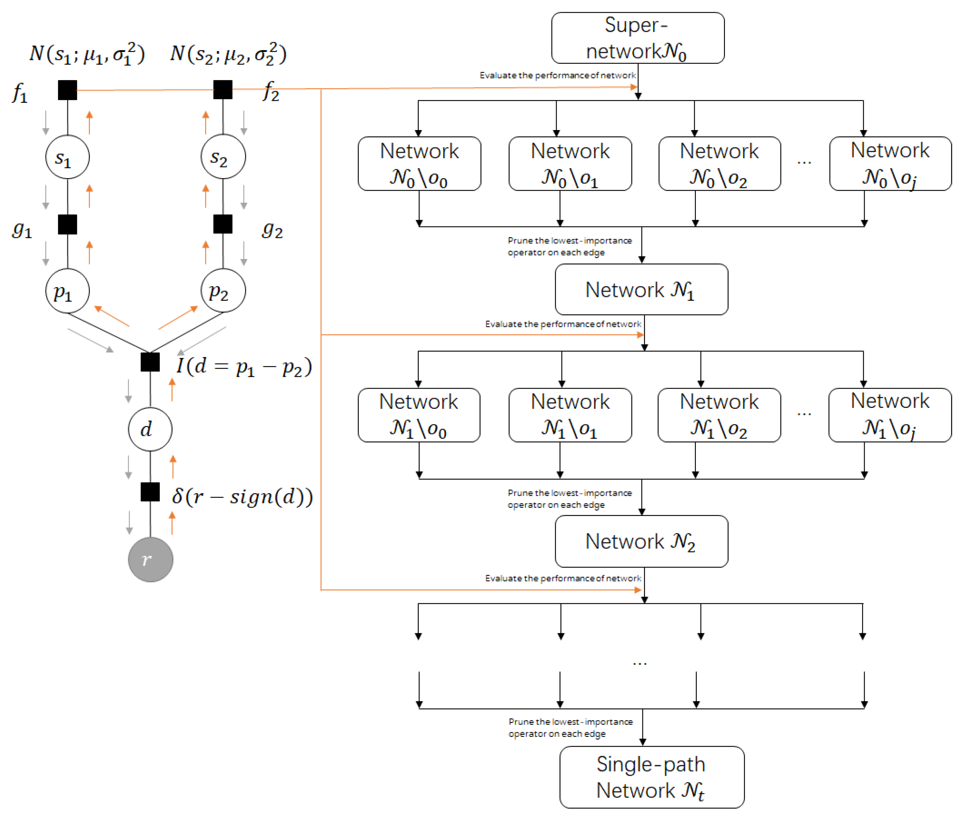
In this section, we utilize the TrueSkill algorithm to refine the evaluation function for assessing network performance. Initially, within the TrueSkill component, we initiate the process by descending along the gray arrow to update the prior probability, as shown in Figure 1. This involves pitting two distinct networks against each other in a competitive scenario. With a priori knowledge regarding the performance of each network, we employ this information to predict the outcome of the competition. Subsequently, by juxtaposing the predicted outcome with the observed result, we iteratively update the posterior probability along the orange arrow. This refined posterior probability is then employed to adjust the weighting of the two indicators within the evaluation function.

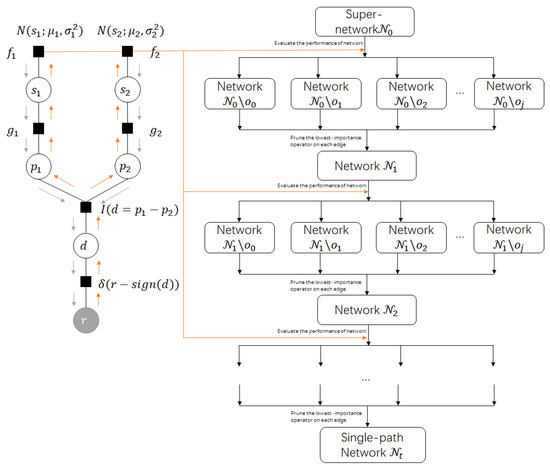
Figure 1. Pipeline: the left part is an algorithm to the evaluate child networks’ performance; the right part is the procedure of the main algorithm. “N” represents the Gaussian distribution, “s” signifies skill, “p” denotes performance, representing actual performance, “d” implies difference, indicating the performance gap between the two parties in competition, and “r” stands for the competing result. Each iteration involves evaluating the performance of the current network without incorporating a specific operation $o_j$, followed by pruning the least-significant operator on each edge. This process continues until we obtain a single-path network that represents the optimal neural network configuration.

Following the TrueSkill refinement, we proceed to execute the pruning algorithm aimed at identifying the optimal single-path network structure. Initially, we initialize the process with a super-network ${\mathcal{N}}_0$, comprising all possible edges and operations. Subsequently, leveraging the evaluation function, we compute the significance of each operation $o_j$ and systematically prune the operation with the lowest significance. This iterative pruning process continues until the network converges to a single-path configuration.

3.1. Training-Free Pruning-Based Architecture Search Algorithm

The primary challenge encountered by the majority of Neural Architecture Search (NAS) methods is substantial training costs involved. To illustrate, envision a network comprised of recurrently structured Directed Acyclic Graph (DAG) cells, with each cell containing a set of E edges. Furthermore, suppose that each edge offers a choice of $\left|O\right|$ distinct candidate operations. In such a scenario, the entirety of the search space would expand exponentially to ${\left|O\right|}^E$. Even if we employ sampling techniques to explore a fraction of this vast search space, represented by a sampling ratio denoted as $\gamma$, the training burden remains formidable. Specifically, to achieve the optimal performance network, one would still need to train approximately ${\gamma \left|O\right|}^E$ distinct architectures. Consequently, the computational demands associated with training such a multitude of architectures pose a significant obstacle in the NAS process.

If a method could be devised to narrow down the search space to $\left|O\right|·E$, the associated searching costs would be notably mitigated, particularly when dealing with extensive search spaces. Additionally, if we could circumvent the necessity of utilizing training results from neural architectures, opting instead for a training-free evaluation method to assess their performance, further savings in computational costs could be achieved.

Moreover, by restricting the exploration to a reduced search space, represented by $\left|O\right|·E$, the computational burden of exploring myriad architectural configurations would be considerably alleviated. This reduction in search space not only enhances efficiency but also streamlines the process of identifying optimal architectures within large-scale search landscapes. Furthermore, the adoption of training-free evaluation methods obviates the need for extensive training iterations, thus significantly reducing the computational overhead associated with training numerous architectures. Consequently, the integration of such methodologies holds the potential to revolutionize the efficiency and scalability of NAS paradigms, facilitating more expedient and cost-effective exploration of architectural design spaces.

In the subsequent sections, we propose a training-free methodology aimed at enhancing the efficiency of conventional NAS approaches. Our approach entails several key steps. Firstly, we endeavor to identify pertinent indicators that are capable of effectively evaluating the quality of the child architectures. These indicators serve as crucial metrics for assessing the performance and efficacy of different architectural configurations. Subsequently, we strive to develop a methodology for effectively balancing these indicators and integrating them cohesively to guide the architecture search process. This involves devising a robust framework for incorporating multiple indicators into the search process, ensuring comprehensive evaluation and optimization of architectural designs. Finally, we introduce a holistic training-free algorithm centered around the concept of pruning, leveraging the identified indicators to inform the pruning process. By integrating these indicators into the pruning algorithm, we aim to refine the search space and expedite the identification of optimal architectural configurations. Through this systematic approach, we seek to streamline the NAS process and mitigate the computational costs associated with traditional training-based methodologies.

3.2. Evaluation of Quality of Child Architectures

In recent research, numerous facets of neural architectures have undergone scrutiny to assess their performance. In our study, we have identified and selected two pivotal indicators to steer our architecture search process: trainability and expressivity. These indicators have been chosen based on their significance in characterizing the effectiveness and efficiency of neural architectures. By focusing on these specific aspects, we aim to develop a comprehensive understanding of architectural design principles and optimize the search process accordingly.

3.2.1. Trainability of Neural Architecture

The ability of a neural network to be optimized using gradient descent [13,14,15] is known as its trainability. Lechao et al. (2019) [16] examined the relationship between the conditioning of the trainable parameters and the trainability of wide networks in their research.

In the finite width NTK, the kernel function is defined as the product of the transpose of the Jacobian of the output of the last layer evaluated at point x, with the Jacobian of the output of the last layer evaluated at point x’. The Jacobian is defined as the derivative of the output of the i-th neuron in the last output layer with respect to the parameter ${\theta }_{\alpha }$, and it is denoted as $J_{i\alpha }\left(x\right)$.

Lechao et al. [16] defined the relationship between the conditioning of the trainable parameters and the trainability of networks as follows:

$${\mu }_t{\left(X_{train}\right)}_i=(I-e^{-\eta {\lambda }_{i}t})Y_{train,i}$$

(1)

the training process can be represented by Equation (1), where ${\mu }_t{\left(X_{train}\right)}_i$ is the training output, I is the identity matrix, $e^{-\eta {\lambda }_{i}t}$ is the exponential function, $\eta$ is the learning rate, and $Y_{train,i}$ is the trainable parameter. The eigenvalues ${\lambda }_i$ of ${\widehat{\Theta }}_{train}$ are used in this equation, and it is hypothesized that the maximum feasible learning rate scales as $\eta \sim {\displaystyle \frac{2}{{\lambda }_0}}$, where ${\lambda }_0$ is the largest eigenvalue. When this scaling is plugged into Equation (1), it can be observed that the smallest eigenvalue will converge at a rate given by $1/{\mathcal{K}}_{\mathcal{N}}$, where

$${\mathcal{K}}_{\mathcal{N}}={\lambda }_0/{\lambda }_m$$

(2)

is the condition number. Therefore, if the condition number of NTK associated with a neural network increases, it will become untrainable, and the condition number is used as a metric for trainability.

It has been observed that when neural networks have large depths, the spectrum of the trainable parameters, ${\Theta }_{(X_{train},Y_{train})}$, typically has one large eigenvalue, ${\lambda }_{max}$, followed by a gap that is much larger than the rest of the spectrum. The condition number of the NTK, ${\mathcal{K}}_{\mathcal{N}}$, is defined as the ratio of the largest eigenvalue to the smallest eigenvalue of a specific neural network $\mathcal{N}$, as shown in Equation (2). This value can be calculated without any gradient descent or labels. The correlation between the condition number of NTK, ${\mathcal{K}}_{\mathcal{N}}$, and the test accuracy of architectures in NAS-Bench-201 has been found to be negative, with a Kendall-tau correlation of −0.42, which suggests that minimizing ${\mathcal{K}}_{\mathcal{N}}$ could lead to finding neural architectures with high performance.

3.2.2. Expressivity by Number of Linear Regions

To ensure a balanced approach in selecting operations for neural architectures, we propose a new evaluation criterion called Expressivity. This criterion is intended to be used in architecture search to complement other evaluation metrics.

Expressivity of a neural network measures its capability to represent complex functions [17,18]. We adopt the approach proposed by Xiong et al. (2020) [19] to evaluate the expressivity of a neural network, which is based on the number of linear regions that a ReLU network can separate. According to Xiong et al. (2020) [19], the expressivity is evaluated by counting the activation patterns and linear regions, which is defined as follows:

Let $\mathcal{N}$ be a ReLU CNN with L hidden convolutional layers. An activation pattern of $\mathcal{N}$ is a function P that maps the set of neurons to 1,–1, meaning that for each neuron z in $\mathcal{N}$, we have $P\left(\mathcal{N}\right)\in 1,-1$. Given a fixed set of parameters $\theta$ in $\mathcal{N}$ and an activation pattern P, we define the region corresponding to P and $\theta$ as follows:

$$\begin{array}{c}\hfill \mathcal{R}(P;\theta )={\displaystyle \{}{X}^0\in {\mathbb{R}}^{n_0^{\left(1\right)}\times n_0^{\left(2\right)}\times d_0}:\\ \hfill z(X^0;\theta )·P\left(z\right)>0,\\ \hfill \forall zaneuronin\mathcal{N}\}\end{array}$$

(3)

where $z(X^0;\theta )$ is the pre-activation of a neuron z. A linear region of $\mathcal{N}$ at $\theta$ is defined as a non-empty set $\mathcal{R}(P;\theta )\ne \varnothing$ for some activation pattern P. The number of linear regions of $\mathcal{N}$ at $\theta$ is represented as follows:

$${\mathcal{R}}_{\mathcal{N},\theta }=\{\#{\mathcal{R}}_{P,\theta }:{\mathcal{R}}_{P,\theta }\ne \varnothing foractivationP\}$$

(4)

Furthermore, we define the ${\mathcal{R}}_{\mathcal{N},\theta }$ as shown in Equation (4) when $\theta$ ranges over $R^{(\#weights+\#bias)}$.

From Equation (3) we can deduce that the number of linear regions ${\mathcal{R}}_{\mathcal{N},\theta }$ reflects the number of distinct activation patterns that the network can separate. We approximate the expected value of ${\mathcal{R}}_{\mathcal{N}}$ by calculating its average:

$$\widehat{\mathcal{R}}\sim {\mathbb{E}}_{\theta }\left[{\mathcal{R}}_{\mathcal{N},\theta }\right]$$

(5)

where $\widehat{\mathcal{R}}$ is an approximation of the expected value of the number of linear regions, and ${\mathbb{E}}_{\theta }$ denotes the expectation over the distribution of parameters $\theta$.

The results of an experiment conducted by Chen et al. [3] showed that there is a positive correlation between the number of linear regions and the test accuracy of neural architectures, as reflected by a Kendall-tau correlation of 0.5. Therefore, it can be inferred that maximizing the number of linear regions can lead to finding architectures with high performance.

3.2.3. Defining the Importance

As demonstrated above, ${\mathcal{K}}_{\mathcal{N}}$ and ${\widehat{R}}_{\mathcal{N}}$ serve as two key indicators for assessing the quality of a neural architecture. ${\mathcal{K}}_{\mathcal{N}}$ exhibits a negative correlation with the architecture’s test accuracy, whereas ${\widehat{R}}_{\mathcal{N}}$ demonstrates a positive correlation with the architecture’s test accuracy. However, in order to ascertain which operation to prune in each iteration, it becomes imperative to devise a method for amalgamating these two indicators into a unified function. This amalgamation will facilitate informed decision-making during the pruning process, enabling the identification of optimal architectural configurations.

3.2.4. Performance Estimation

We can clearly see that ${\mathcal{K}}_{\mathcal{N}}$ and ${\widehat{R}}_{\mathcal{N}}$ favor different operations on NAS-Bench-201, which is shown in Figure 2. They both employ $conv3\times 3$ with a large ratio, but  ${\mathcal{K}}_{\mathcal{N}}$ favors the skip-connect operation compared with the $conv1\times 1$ operation, while ${\widehat{R}}_{\mathcal{N}}$ favors the $conv1\times 1$ operation with a much higher ratio compared with the skip-connect operation. Then, if there is a conflict where an operation that ${\widehat{R}}_{\mathcal{N}}$ favors is not what ${\mathcal{K}}_{\mathcal{N}}$ favors, how can we determine which operation should be pruned?

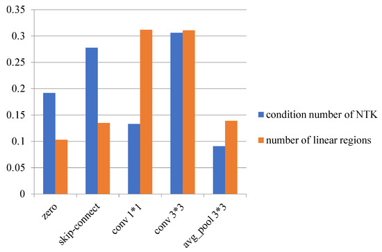
Figure 2. The distribution of the preferences of ${\mathcal{K}}_{\mathcal{N}}$ and $R_{\mathcal{N}}$ (conducted by TE-NAS [3]). ${\mathcal{K}}_{\mathcal{N}}$ and $R_{\mathcal{N}}$ favor different operations on NAS-Bench-201.

Chen et al. (2021) [3] made a rough trade-off that they directly attributed to using the two relative rankings of $\Delta {\mathcal{K}}_{t,o_j}$ and $\Delta {\widehat{R}}_{t,o_j}$ as the selection criterion. More specifically, they sorted the $\Delta {\mathcal{K}}_{t,o_j}$ in descending order and $\Delta {\widehat{R}}_{t,o_j}$ in ascending order. The higher the $\Delta {\mathcal{K}}_{t,o_j}$ value, the more likely they would prune $o_j$, and the lower the $\Delta {\widehat{R}}_{t,o_j}$ value, the more likely they would prune $o_j$. They pruned the operation with the lowest sum rank of $\Delta {\mathcal{K}}_{t,o_j}$ and $\Delta {\widehat{R}}_{t,o_j}$. This indeed works in some specific cases, but this algorithm ignores two important facts: (1) trainability may be not as important as expressivity; and (2) the preferences of $\Delta {\mathcal{K}}_{t,o_j}$ and $\Delta {\widehat{R}}_{t,o_j}$ may be different on different types of datasets; for example, a neural network that performs well on an image dataset may not provide a good neural architecture if trained with words.

We assume that ${\mathcal{K}}_{\mathcal{N}}$ and ${\widehat{R}}_{\mathcal{N}}$ have different importance coefficients based on the quality of the neural architecture. ${\lambda }_{\mathcal{K}}$ and ${\lambda }_R$ can be seen as the importance of ${\mathcal{K}}_{\mathcal{N}}$ and ${\widehat{R}}_{\mathcal{N}}$ to the performance of a neural network. Given the importance of ${\mathcal{K}}_{\mathcal{N}}$ and ${\widehat{R}}_{\mathcal{N}}$, we simplify the combined function as follows:

$${\mathcal{F}}_{\mathcal{N}}={\lambda }_{\mathcal{K}}{\mathcal{K}}_{\mathcal{N}}+{\lambda }_R{\widehat{R}}_{\mathcal{N}}$$

(6)

We use ${\mathcal{F}}_{\mathcal{N}}$ to estimate the quality of $\mathcal{N}$.

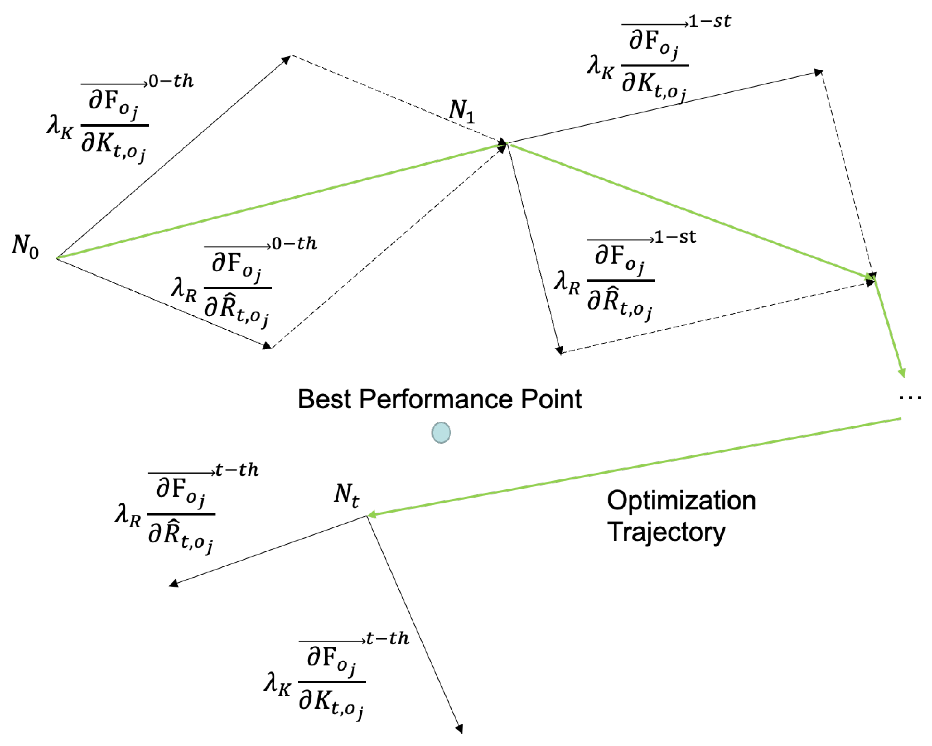
Understanding Equation (6) entails consideration of a neural architecture ${\mathcal{N}}_0$ that is composed of multiple candidate operations on edges. If we prune one operation $o_j$ from ${\mathcal{N}}_0$, we use $\Delta {\mathcal{F}}_{o_j}$ to represent the variation in ${\mathcal{N}}_0$’s estimate quality. The estimation of ${\mathcal{N}}_0$ is related to two indicators: ${\mathcal{K}}_{\mathcal{N}}$ and ${\widehat{R}}_{\mathcal{N}}$. Then, we can use a 2D plane to show the estimation state of ${\mathcal{N}}_0$ in Figure 3.

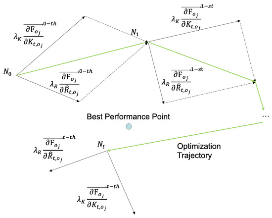
Figure 3. Training phase elaboration: The algorithm starts with super-network ${\mathcal{N}}_0$, then it is optimized under the vector sum of ${\lambda }_{\mathcal{K}}\overrightarrow{{\displaystyle \frac{\partial {\mathcal{F}}_{o_j}}{\partial {\mathcal{K}}_{t,o_j}}}}$ and ${\lambda }_R\overrightarrow{{\displaystyle \frac{\partial {\mathcal{F}}_{o_j}}{\partial {\widehat{R}}_{t,o_j}}}}$. ${\lambda }_{\mathcal{K}}$ and ${\lambda }_R$ are obtained from Algorithm 1. Iteratively, the stop point ${\mathcal{N}}_t$ will approach the best performance point.

Let us write a total derivative of $\Delta {\mathcal{F}}_{o_j}$ as follows:

$$\overrightarrow{\Delta {\mathcal{F}}_{o_j}}={\lambda }_{\mathcal{K}}·(\Delta {\mathcal{K}}_{t,o_j}·\overrightarrow{{\displaystyle \frac{\partial {\mathcal{F}}_{o_j}}{\partial {\mathcal{K}}_{t,o_j}}}})+{\lambda }_R·(\Delta {\widehat{R}}_{t,o_j}·\overrightarrow{{\displaystyle \frac{\partial {\mathcal{F}}_{o_j}}{\partial {\widehat{R}}_{t,o_j}}}})$$

(7)

$\overrightarrow{{\displaystyle \frac{\partial {\mathcal{F}}_{o_j}}{\partial {\mathcal{K}}_{t,o_j}}}}$ and $\overrightarrow{{\displaystyle \frac{\partial {\mathcal{F}}_{o_j}}{\partial {\widehat{R}}_{t,o_j}}}}$ are two independent unit vectors pointing in two directions. Since we do not know the scale of each direction, we use two parameters ${\lambda }_{\mathcal{K}}$ and ${\lambda }_R$ to estimate them. The closer ${\lambda }_{\mathcal{K}}$ and ${\lambda }_R$ are to their ground truth, the less bias we would suffer during the process of pruning the candidate operations.

We consider two neural architectures, $\mathcal{N}$ and ${\mathcal{N}}^{\prime }$, which have at least one different operation on the same edge. We can use the combined function ${\mathcal{F}}_{\mathcal{N}}$ to evaluate the quality of $\mathcal{N}$ and ${\mathcal{N}}^{\prime }$ based on our current priori estimation of ${\lambda }_{\mathcal{K}}$ and ${\lambda }_R$ as follows:

$$\begin{array}{c}\hfill {\mathcal{F}}_{\mathcal{N}}={\lambda }_{\mathcal{K}}{\mathcal{K}}_{\mathcal{N}}+{\lambda }_R{\widehat{R}}_{\mathcal{N}}\\ \hfill {\mathcal{F}}_{{\mathcal{N}}^{\prime }}={\lambda }_{\mathcal{K}}{\mathcal{K}}_{{\mathcal{N}}^{\prime }}+{\lambda }_R{\widehat{R}}_{{\mathcal{N}}^{\prime }}\end{array}$$

(8)

3.2.5. Update the Importance

We initiate a competitive scenario wherein two neural architectures engage in a head-to-head comparison to ascertain the alignment between their actual performance and our current estimation. Subsequently, we leverage the outcome of this competition to iteratively refine and update our estimation in a reverse manner. This iterative process enables us to validate the accuracy of our initial estimation by directly observing the comparative performance of the competing architectures. Through this feedback loop, we continually enhance the precision and reliability of our estimations, ensuring they remain reflective of the practical performance exhibited by the neural architectures. If ${\mathcal{F}}_{\mathcal{N}}>{\mathcal{F}}_{{\mathcal{N}}^{\prime }}$, then we could deduce that $\mathcal{N}$ should perform better than ${\mathcal{N}}^{\prime }$. We simplify the inequation ${\mathcal{F}}_{\mathcal{N}}>{\mathcal{F}}_{{\mathcal{N}}^{\prime }}$ as follows:

$$\begin{array}{c}\hfill ({\lambda }_{\mathcal{K}}{\mathcal{K}}_{\mathcal{N}}+{\lambda }_R{\widehat{R}}_{\mathcal{N}})-\\ \hfill ({\lambda }_{\mathcal{K}}{\mathcal{K}}_{{\mathcal{N}}^{\prime }}+{\lambda }_R{\widehat{R}}_{{\mathcal{N}}^{\prime }})>0\end{array}$$

(9)

$${\lambda }_{\mathcal{K}}({\mathcal{K}}_{\mathcal{N}}-{\mathcal{K}}_{{\mathcal{N}}^{\prime }})>-{\lambda }_R({\widehat{R}}_{\mathcal{N}}-{\widehat{R}}_{{\mathcal{N}}^{\prime }})$$

(10)

According to Inequation (10), comparing ${\lambda }_{\mathcal{K}}({\mathcal{K}}_{\mathcal{N}}-{\mathcal{K}}_{{\mathcal{N}}^{\prime }})$ and $-{\lambda }_R({\widehat{R}}_{\mathcal{N}}-{\widehat{R}}_{{\mathcal{N}}^{\prime }})$ is equivalent to comparing ${\mathcal{F}}_{\mathcal{N}}$ and ${\mathcal{F}}_{{\mathcal{N}}^{\prime }}$, which means we can use the competence result to update ${\lambda }_{\mathcal{K}}$ and ${\lambda }_R$, where $({\mathcal{K}}_{\mathcal{N}}-{\mathcal{K}}_{{\mathcal{N}}^{\prime }})$ and $-({\widehat{R}}_{\mathcal{N}}-{\widehat{R}}_{{\mathcal{N}}^{\prime }})$ can be calculated as constants in each competence. By making them compete with each other multiple times, we could determine their importance more precisely. We propose a new method to combine ${\mathcal{K}}_{\mathcal{N}}$ and ${\widehat{R}}_{\mathcal{N}}$ with their importance ${\lambda }_{\mathcal{K}}$ and ${\lambda }_R$ by applying the TrueSkill algorithm given in Algorithm 1.

In Algorithm 1, $\beta$ is a constant value used to measure the instability of the performance of two competitors, and v and w are the additive and multiplicative correction terms for the mean and variance of a (doubly) truncated Gaussian, respectively. This is shown as follows:

$$V_{\mathbb{1}|·|>ϵ}(t,ϵ):={\displaystyle \frac{N(t-ϵ)}{\Phi (t-ϵ)}}$$

(11)

$$\begin{array}{cc}\hfill & W_{\mathbb{1}|·|>ϵ}(t,ϵ):=V_{\mathbb{1}|·|>ϵ}^2\hfill \\ & +{\displaystyle \frac{(ϵ-t)·N(ϵ-t)+(ϵ+t)·N(ϵ+t)}{\Phi (ϵ-t)-\Phi (ϵ+t)}}\hfill \end{array}$$

(12)

While the ELO algorithm remains a widely adopted method for evaluating performance, we have opted to employ the TrueSkill algorithm in our approach for several reasons:

• TrueSkill can handle fair status.
• TrueSkill can handle multi-player situations; although two factors are taken into consideration, we may use more factors in the future.
• TrueSkill has a rigorous theory foundation.
• TrueSkill converges faster than ELO.
• TrueSkill requires little fine-tuning of hyperparameters.

Algorithm 1 Measurement of ${\mathcal{K}}_{\mathcal{N}}$ and ${\widehat{R}}_{\mathcal{N}}$

Input: Begin with two different neural architectures ${\mathcal{N}}_1$ and ${\mathcal{N}}_2$, current estimation ${\lambda }_{\mathcal{K}},{\sigma }_{\mathcal{K}},{\lambda }_R,{\sigma }_R$, for importance of ${\mathcal{K}}_{\mathcal{N}}$ and ${\widehat{R}}_{\mathcal{N}}$ Initialization: $r_1=get\_accuracy\left({\mathcal{N}}_1\right)$; $r_2=get\_accuracy\left({\mathcal{N}}_2\right)$; $r=sign(r_1-r_2)$; if $r==1$ then ${\mathcal{N}}_1$ wins, others ${\mathcal{N}}_2$ wins Let ${\mu }_1={\lambda }_{\mathcal{K}}({\mathcal{K}}_{{\mathcal{N}}_1}-{\mathcal{K}}_{{\mathcal{N}}_2})$, ${\mu }_2={\lambda }_R(R_{{\mathcal{N}}_2}-R_{{\mathcal{N}}_1})$, ${\sigma }_1={\sigma }_{\mathcal{K}}$, ${\sigma }_2={\sigma }_R$  Based on the competing result r, update ${\mu }_1$ and ${\mu }_2$ as:  ${\mu }_{winner}$$+=$${\displaystyle \frac{{\sigma }_{winner}^2}{c}}·v({\displaystyle \frac{{\mu }_{winner}-{\mu }_{loser}}{c}},{\displaystyle \frac{\epsilon }{c}})$  ${\mu }_{loser}$$-=$${\displaystyle \frac{{\sigma }_{loser}^2}{c}}·v({\displaystyle \frac{{\mu }_{winner}-{\mu }_{loser}}{c}},{\displaystyle \frac{\epsilon }{c}})$  ${\sigma }_{winner}^2$$\ast =$$[1-{\displaystyle \frac{{\sigma }_{winner}^2}{c^2}}·w({\displaystyle \frac{{\mu }_{winner}-{\mu }_{loser}}{c}},{\displaystyle \frac{\epsilon }{c}})]$  ${\sigma }_{loser}^2$$\ast =$$[1-{\displaystyle \frac{{\sigma }_{loser}^2}{c^2}}·w({\displaystyle \frac{{\mu }_{winner}-{\mu }_{loser}}{c}},{\displaystyle \frac{\epsilon }{c}})]$  update ${\lambda }_{\mathcal{K}},{\sigma }_{\mathcal{K}},{\lambda }_R{\sigma }_R$ as:  ${\lambda }_{\mathcal{K}}={\displaystyle \frac{{\mu }_1}{{\mathcal{K}}_{{\mathcal{N}}_1}-{\mathcal{K}}_{{\mathcal{N}}_2}}}$  ${\lambda }_R={\displaystyle \frac{{\mu }_2}{R_{{\mathcal{N}}_2}-R_{{\mathcal{N}}_1}}}$  ${\sigma }_{\mathcal{K}}={\sigma }_1$  ${\sigma }_R={\sigma }_2$  $c^2=2{\beta }^2+{\sigma }_{winner}^2+{\sigma }_{loser}^2$  return  ${\lambda }_{\mathcal{K}},{\sigma }_{\mathcal{K}},{\lambda }_R,{\sigma }_R$  $-get\_accuracy\left(\mathcal{N}\right):$ train the neural architecture $\mathcal{N}$ with the dataset and return the final test accuracy.

3.2.6. Pruning Network

Traditional network pruning typically requires pre-trained weights and specific strategies to ensure successful learning of the pruned structure. However, recent advancements in pruning-from-scratch, as demonstrated in works such as [20,21], have shown that the structure of pruned models can be directly learned from randomly initialized weights without sacrificing performance. This breakthrough enables network pruning without the need for pre-trained weights, streamlining the pruning process and reducing dependencies on external resources.

Inspired by the prune-from-scratch approach, we extend our methodology to propose a pruning-operation-by-importance NAS method aimed at reducing the search space and enhancing search efficiency. In our approach, we iteratively prune one candidate operation with the least importance on each edge in a single round. This strategy effectively reduces the algorithmic complexity from ${\left|O\right|}^E$ to $\left|O\right|·E$. We encapsulate our training-free and pruning-based algorithm, referred to as TTNAS, in Algorithm 2. This algorithmic framework streamlines the search process and facilitates efficient exploration of architectural configurations, leading to improved performance and computational efficiency.

Algorithm 2 Training-free TrueSkill NAS

Input: ${\lambda }_{\mathcal{K}}$,${\lambda }_R$, super-network ${\mathcal{N}}_0$ stacked by cells, each cell has E edges, each edge has $\left|O\right|$ candidate operations Initialization: step $t=0$ 1: while ${\mathcal{N}}_t$ is not a single-path network do 2:     for each operation $o_j$ in ${\mathcal{N}}_t$ do 3:         $\Delta {\mathcal{K}}_{t,o_j}=-({\mathcal{K}}_{{\mathcal{N}}_t}-{\mathcal{K}}_{{\mathcal{N}}_t}\setminus o_j)$ 4:         $\Delta {\widehat{R}}_{t,o_j}=-(R_{{\mathcal{N}}_t}-R_{{\mathcal{N}}_t}\setminus o_j)$ 5:     end for 6:     $\Delta {\mathcal{F}}_{o_j}={\lambda }_{\mathcal{K}}·\Delta {\mathcal{K}}_{t,o_j}+{\lambda }_R·\Delta {\widehat{R}}_{t,o_j}$ 7:     ${\mathcal{N}}_{t+1}={\mathcal{N}}_t$ 8:     for each edge $e_i,i=1,\dots ,E$ do 9:         $j^{\ast }={argmin}_j\{\Delta {\mathcal{F}}_{o_j}:o_j\in e_i\}$ 10:       ${\mathcal{N}}_{t+1}={\mathcal{N}}_{t+1}\setminus o_{j^{\ast }}$ 11:     end for 12:     $t=t+1$ 13: end while 14: return pruned single-path network ${\mathcal{N}}_t$

In Algorithm 2, we start with a super-network ${\mathcal{N}}_0$ stacked by multiple repeated cells [22], which is composed of all possible edges and candidate operations. In each outer loop, we prune one operation with the least importance to the whole architecture ${\mathcal{N}}_t$ on each edge until ${\mathcal{N}}_t$ is a single-path network. In the inner loop, we calculate the change in ${\mathcal{K}}_{\mathcal{N}}$ and ${\widehat{R}}_{\mathcal{N}}$ before and after pruning each candidate operation, and we evaluate its importance with $\Delta {\mathcal{F}}_{o_j}$, and prune the candidate operation with the lowest importance on each edge.

The entire pruning process exhibits exceptional speed and efficiency. As we will illustrate in subsequent sections, our approach is methodical and adaptable, requiring minimal modifications for application across diverse architectural spaces and datasets. The prune-operation-by-importance mechanism employed in our methodology can be seamlessly extended beyond the indicators ${\mathcal{K}}_{\mathcal{N}}$ and ${\widehat{R}}_{\mathcal{N}}$. This extension holds promise for incorporating additional indicators or network properties, thereby enhancing the versatility and applicability of our approach in various contexts. Furthermore, the scalability of our methodology ensures its effectiveness across different domains and datasets, underscoring its potential as a robust solution for efficient neural architecture refinement.

3.3. TTNAS with Multiple Indicators

In this section, we introduce an indicator for evaluating the performance of neural architectures, namely discriminability. This section is structured as follows: First, we will elucidate the concept of discriminability in the context of neural networks and detail the methodology for calculating this metric. Following this, we will explore how the TrueSkill algorithm can be employed to ascertain the relative importance of discriminability within the evaluation framework. We will then discuss how to integrate discriminability with existing indicators to provide a comprehensive assessment of neural network performance. Lastly, we will outline how the prune-based search strategy of the training-free TrueSkill NAS can be adapted to incorporate this new evaluation method, thereby enhancing the search process for optimal network architectures.

3.3.1. Introduction to Discriminability

Discriminability, within the context of neural network performance evaluation, pertains to the capability of a network to differentiate between distinct classes or inputs with a high degree of accuracy. This concept is crucial, as it directly influences the network’s ability to perform well in classification tasks and other applications requiring precise distinctions. Explicitly defined, a robust and flexible network should not only be adept at discerning local linear operators for each individual data point but also exhibit consistency in its outputs for similar data points. This dual capability ensures that the network can handle complex patterns and maintain coherence in its decision-making processes.

The ideal scenario in neural network evaluation would involve an untrained network that exhibits low correlations between different data points. Specifically, data points belonging to the same category should be clustered closely together, indicating a high degree of similarity within categories. This clustering effect would facilitate the network’s learning process during training, as it would encounter fewer challenges in distinguishing between different categories. Consequently, the network would be able to learn and generalize more effectively, leading to improved performance metrics.

In this ideal scenario, the network’s ability to distinguish between similar data points within the same category is balanced with its capacity to differentiate between distinct categories. This balance is essential for achieving high discriminability, as it ensures that the network can accurately classify new, unseen data points based on the patterns it has learned during training. The importance of this balance cannot be overstated, as it directly impacts the network’s overall performance and reliability in real-world applications.

To further elucidate the concept of discriminability, consider a neural network tasked with classifying images of different animals. A network with high discriminability would be able to accurately distinguish between images of cats and dogs, even if the images differ only in subtle details. Moreover, the network should consistently classify images of similar animals (e.g., different breeds of dogs) correctly, demonstrating its ability to handle fine-grained distinctions. This level of performance is indicative of a well-trained network that has learned to recognize and differentiate between various patterns with high accuracy.

3.3.2. Assessing the Discriminability of Neural Networks

We base our approach on a fundamental assumption: different networks can be effectively compared by evaluating their behavior using local linear operators at various data points. This assumption stems from the premise that the local behavior of neural networks can provide valuable insights into their overall performance and capabilities. By examining how networks respond to small perturbations in the input space, we can gain a deeper understanding of their decision-making processes and identify key differences between various network architectures.

To do this, we define a linear map, $w_i=f\left(x_i\right)$, which maps the input $x_i\in {\mathbb{R}}^D$ through the network $f\left(x_i\right)$, where $x_i$ represents an image that belongs to a batch X, and D is the input dimension. Then, the linear map can be computed as follows:

$$Jacobian{w}_i={\displaystyle \frac{\partial f\left(x_i\right)}{\partial x_i}}$$

In order to evaluate how a network behaves with different data points, we calculate the Jacobian matrix $w_i$ for different data points of the batch, $i=\{1,2,3,\dots ,N\}$:

$$J={\left({\displaystyle \frac{\partial f\left(x_1\right)}{\partial x_1}}{\displaystyle \frac{\partial f\left(x_2\right)}{\partial x_2}}{\displaystyle \frac{\partial f\left(x_3\right)}{\partial x_3}}\dots {\displaystyle \frac{\partial f\left(x_N\right)}{\partial x_N}}\right)}^T$$

The Jacobian Matrix J contains information about the network output with respect to the input for several data points. We can then evaluate how points belonging to the same class correlate with each other.

To evaluate the discriminability of neural networks, we assess the correlation of J values with respect to their respective classes by computing a covariance matrix for each class present in J. This approach allows us to quantify the relationships between the Jacobian values and the class labels, thereby providing insights into the network’s ability to distinguish between different classes.

$$C_c=(J-M_{J_c}){(J-M_{J_c})}^T$$

where $M_J$ is the matrix with elements:

$${\left(M_{J_c}\right)}_{ij}={\displaystyle \frac{1}{N}}\sum _{n\in \{1,2,\dots ,N\},x_i\in \mathrm{class}c}{J}_{i,n}$$

where c represents the class, $c\in \{1,2,\dots ,C\}$, and C is the number of classes present in the batch.

Then, it is possible to calculate the correlation matrix per class $P_{J_c}$ for each covariance matrix $C_{J_c}$:

$${\left(P_{J_c}\right)}_{i,j}={\displaystyle \frac{{\left(C_{J_c}\right)}_{i,j}}{\sqrt{{\left(C_{J_c}\right)}_{i,i}\ast {\left(C_{J_c}\right)}_{j,j}}}}$$

Each individual correlation matrix provides a comprehensive analysis of the behavior of an untrained network across different classes. This analysis serves as a critical indicator of the local linear operators’ capability to distinguish between various class characteristics.

To facilitate the comparison among the various individual correlation matrices, which may exhibit varying sizes due to the differing number of data points per class, each matrix is evaluated separately:

$$E_C=\left\{\begin{array}{cc}\sum _{i=0}^N\sum _{j=0}^{N}log\left(\right|{\left(P_{J_C}\right)}_{i,j}|+\epsilon ),\hfill & \mathrm{if}C<\mathrm{constant}\hfill \\ {\displaystyle \frac{{\sum }_{i=0}^N{\sum }_{j=0}^{N}log\left(\right|{\left(P_{J_C}\right)}_{i,j}|+\epsilon )}{\left|\right|P_{J_C}\left|\right|}},\hfill & \mathrm{otherwise}\hfill \end{array}\right.$$

where $\epsilon$ is a small constant. We denote $\left|\right|P_{J_C}\left|\right|$ as the number of elements of the set $P_{J_C}$.

Finally, we use S to evaluate the discriminability of neural networks:

$$S=\left\{\begin{array}{cc}\sum _{t=0}^C\left|E_t\right|,\hfill & \mathrm{if}C<\mathrm{constant}\hfill \\ {\displaystyle \frac{{\sum }_{i=0}^C{\sum }_{j=i}^C|E_i-E_j|}{\left|\right|E\left|\right|}},\hfill & \mathrm{otherwise}\hfill \end{array}\right.$$

where E is the vector containing all correlation matrices’ scores.

3.3.3. Evaluation Method with Three Indicators

With an additional indicator included, we have three indicators: trainability ${\mathcal{K}}_{\mathcal{N}}$, expressivity ${\widehat{R}}_{\mathcal{N}}$, and discriminability ${\mathcal{S}}_{\mathcal{N}}$.

We define the performance of three different neural networks, ${\mathcal{N}}_1,{\mathcal{N}}_2$, and ${\mathcal{N}}_3$, as follows:

$$\begin{array}{cc}\hfill {\mathcal{F}}_1& ={\lambda }_{\mathcal{K}}·\Delta {\mathcal{K}}_{{\mathcal{N}}_1}+{\lambda }_R·\Delta {\widehat{R}}_{{\mathcal{N}}_1}+{\lambda }_S·\Delta {\mathcal{S}}_{{\mathcal{N}}_1}\hfill \\ \hfill {\mathcal{F}}_2& ={\lambda }_{\mathcal{K}}·\Delta {\mathcal{K}}_{{\mathcal{N}}_2}+{\lambda }_R·\Delta {\widehat{R}}_{{\mathcal{N}}_2}+{\lambda }_S·\Delta {\mathcal{S}}_{{\mathcal{N}}_2}\hfill \\ \hfill {\mathcal{F}}_3& ={\lambda }_{\mathcal{K}}·\Delta {\mathcal{K}}_{{\mathcal{N}}_3}+{\lambda }_R·\Delta {\widehat{R}}_{{\mathcal{N}}_3}+{\lambda }_S·\Delta {\mathcal{S}}_{{\mathcal{N}}_3}\hfill \end{array}$$

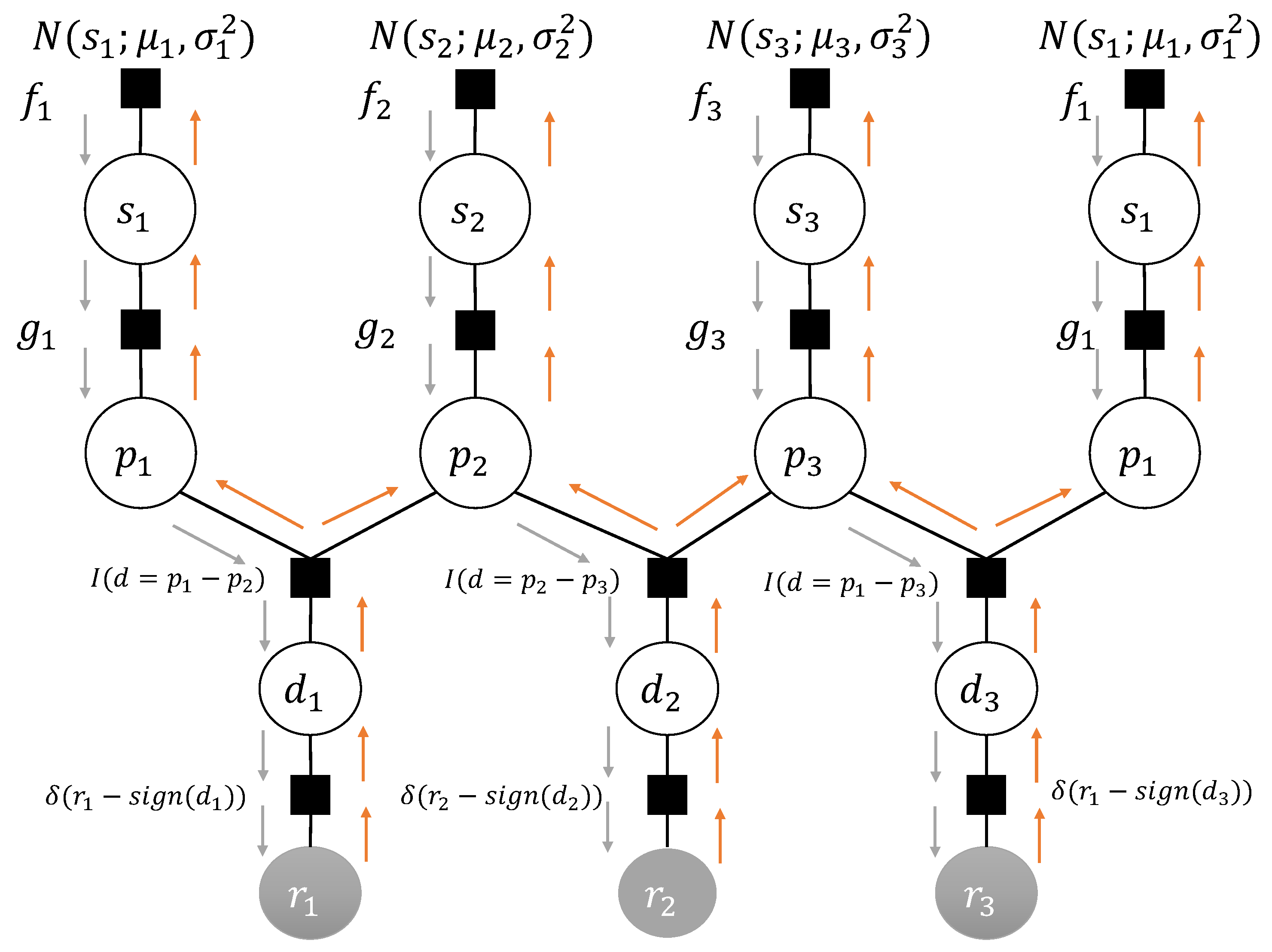
We let the three neural networks compete with each other. An overview of the TrueSkill algorithm with the three indicators is shown in Figure 4.

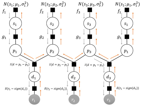
Figure 4. “N” represents the Gaussian distribution, “s” signifies skill, denoting the ability value of each player, “p” denotes performance, representing actual performance, “d” implies difference, indicating the performance gap between the two parties in competition, and “r” stands for result, signifying the outcome of the competition.

Once two neural networks, ${\mathcal{N}}_1$ and ${\mathcal{N}}_2$, have competed, we fix one of the indicators and update the other two indicators.

Combined with the TrueSkill algorithm, we can update the equations of these three indicators:

Let ${\mu }_1={\lambda }_{\mathcal{K}}(\Delta {\mathcal{K}}_{{\mathcal{N}}_1}-\Delta {\mathcal{K}}_{{\mathcal{N}}_2})$, ${\mu }_2=-[{\lambda }_R(\Delta {\widehat{\mathcal{R}}}_{{\mathcal{N}}_1}-\Delta {\widehat{\mathcal{R}}}_{{\mathcal{N}}_2})+C_S]$, $C_S={\lambda }_S(\Delta S_{{\mathcal{N}}_1}-\Delta S_{{\mathcal{N}}_2})$, ${\sigma }_1={\sigma }_{\mathcal{K}}$, ${\sigma }_2={\sigma }_R$, where $C_S$ is a constant. According to the competition results of neural networks ${\mathcal{N}}_1$ and ${\mathcal{N}}_2$, we update ${\mu }_1$, ${\mu }_2$, ${\sigma }_1$, ${\sigma }_2$ as follows:

$${\mu }_{winner}+={\displaystyle \frac{{\sigma }_{winner}^2}{c}}·v\left({\displaystyle \frac{{\mu }_{winner}-{\mu }_{loser}}{c}},{\displaystyle \frac{\epsilon }{c}}\right)$$

$${\mu }_{loser}={\displaystyle \frac{{\sigma }_{loser}^2}{c}}·v\left({\displaystyle \frac{{\mu }_{winner}-{\mu }_{loser}}{c}},{\displaystyle \frac{\epsilon }{c}}\right)$$

$${\sigma }_{winner}^2\ast =\left[1-{\displaystyle \frac{{\sigma }_{winner}^2}{c^2}}·\omega \left({\displaystyle \frac{{\mu }_{winner}-{\mu }_{loser}}{c}},{\displaystyle \frac{\epsilon }{c}}\right)\right]$$

$${\sigma }_{loser}^2\ast =\left[1-{\displaystyle \frac{{\sigma }_{winner}^2}{c^2}}·\omega \left({\displaystyle \frac{{\mu }_{winner}-{\mu }_{loser}}{c}},{\displaystyle \frac{\epsilon }{c}}\right)\right]$$

After updating ${\mu }_1$, ${\mu }_2$, ${\sigma }_1$, ${\sigma }_2$, we can update ${\lambda }_{\mathcal{K}}$ and ${\lambda }_R$ as follows:

$${\lambda }_{\mathcal{K}}={\displaystyle \frac{{\mu }_1}{\Delta {\mathcal{K}}_{{\mathcal{N}}_1}-\Delta {\mathcal{K}}_{{\mathcal{N}}_2}}}$$

$${\lambda }_R={\displaystyle \frac{{\mu }_2+C_S}{\Delta {\widehat{\mathcal{R}}}_{{\mathcal{N}}_2}-\Delta {\widehat{\mathcal{R}}}_{{\mathcal{N}}_1}}}$$

$${\sigma }_{\mathcal{K}}={\sigma }_1$$

$${\sigma }_R={\sigma }_2$$

$$C_{\mathcal{K},R}=2{\beta }^2+{\sigma }_{winner}^2+{\sigma }_{loser}^2$$

Similarly, we update ${\widehat{R}}_{\mathcal{N}}$ and $S_{\mathcal{N}}$ via the competition between two neural networks, ${\mathcal{N}}_2$ and ${\mathcal{N}}_3$:

Let

$$\begin{array}{cc}\hfill {\mu }_3& ={\lambda }_R(\Delta {\widehat{R}}_{{\mathcal{N}}_2}-\Delta {\widehat{R}}_{{\mathcal{N}}_3}),\hfill \\ \hfill {\mu }_4& =-[{\lambda }_s(\Delta S_{{\mathcal{N}}_2}-\Delta S_{{\mathcal{N}}_3})+C_{\mathcal{K}}],\hfill \\ \hfill C_{\mathcal{K}}& ={\lambda }_{\mathcal{K}}(\Delta {\mathcal{K}}_{{\mathcal{N}}_2}-\Delta {\mathcal{K}}_{{\mathcal{N}}_3}),\hfill \\ \hfill {\sigma }_3& ={\sigma }_R,\hfill \\ \hfill {\sigma }_4& ={\sigma }_S,\hfill \end{array}$$

where $C_{\mathcal{K}}$ is a constant. According to the competition results of two neural networks, ${\mathcal{N}}_2$ and ${\mathcal{N}}_3$, we update ${\mu }_3,{\mu }_4,{\sigma }_3,{\sigma }_4$.

After updating ${\mu }_3,{\mu }_4,{\sigma }_3,{\sigma }_4$, we can update ${\lambda }_{\mathcal{K}}$ and ${\lambda }_R$ as follows:

$$\begin{array}{cc}\hfill {\lambda }_R& ={\displaystyle \frac{{\mu }_3}{\Delta {\widehat{R}}_{{\mathcal{N}}_2}-\Delta {\widehat{R}}_{{\mathcal{N}}_3}}}\hfill \\ \hfill {\lambda }_S& ={\displaystyle \frac{\Delta S_{{\mathcal{N}}_2}-\Delta S_{{\mathcal{N}}_2}}{{\mu }_4+C_S}}\hfill \\ \hfill {\sigma }_R& ={\sigma }_3\hfill \\ \hfill {\sigma }_S& ={\sigma }_4\hfill \\ \hfill C_{R,S}& =2{\beta }^2+{\sigma }_{winner}^2+{\sigma }_{loser}^2\hfill \end{array}$$

We update ${\mathcal{K}}_{\mathcal{N}}$ and $S_{\mathcal{N}}$ via the competition of two neural networks, ${\mathcal{N}}_1$ and ${\mathcal{N}}_3$:

Let ${\mu }_5={\lambda }_{\mathcal{K}}(\Delta {\mathcal{K}}_{{\mathcal{N}}_1}-\Delta {\mathcal{K}}_{{\mathcal{N}}_3}),{\mu }_6=-[{\lambda }_s(\Delta S_{{\mathcal{N}}_1}-\Delta S_{{\mathcal{N}}_3})+C_R]$, $C_R={\lambda }_R(\Delta {\widehat{R}}_{{\mathcal{N}}_1}-\Delta {\widehat{R}}_{{\mathcal{N}}_3})$, ${\sigma }_5={\sigma }_{\mathcal{K}},{\sigma }_6={\sigma }_s$, where $C_{\mathcal{K}}$ is a constant. According to the competition results of two neural networks, ${\mathcal{N}}_1$ and ${\mathcal{N}}_3$, we update ${\mu }_5,{\mu }_6,{\sigma }_5,{\sigma }_6$ with the equations.

After updating ${\mu }_5,{\mu }_6,{\sigma }_5,{\sigma }_6$, we can update ${\lambda }_{\mathcal{K}}$ and ${\lambda }_s$ as follows:

$${\lambda }_{\mathcal{K}}={\displaystyle \frac{{\mu }_5}{\Delta {\mathcal{K}}_{{\mathcal{N}}_1}-\Delta {\mathcal{K}}_{{\mathcal{N}}_3}}}$$

$${\lambda }_s={\displaystyle \frac{{\mu }_6+C_R}{\Delta S_{{\mathcal{N}}_3}-\Delta S_{{\mathcal{N}}_1}}}$$

$${\sigma }_{\mathcal{K}}={\sigma }_5$$

$${\sigma }_s={\sigma }_6$$

$$C_{\mathcal{K},S}=2{\beta }^2+{\sigma }_{winner}^2+{\sigma }_{loser}^2$$

With three indicators included in the TrueSkill training-free NAS, we first update the measurement of these three indicators, which are ${\lambda }_K,{\lambda }_R,{\lambda }_S$.

After updating ${\lambda }_K,{\lambda }_R,{\lambda }_S$, we use them to evaluate the performance of the neural network:

$${\mathcal{F}}_N={\lambda }_K·\Delta {\mathcal{K}}_N+{\lambda }_R·\Delta {\widehat{R}}_N+{\lambda }_S·\Delta S_N$$

3.3.4. Prune-Based Search Strategy with Three Indicators

As the additional indicator added into consideration, we summarize the evaluation method based on these indicators. We can easily conclude the following points regarding the prune-based search algorithm:

Similar to the training-free true-skill NAS in Algorithm 3, we initiate with a super-network ${\mathcal{N}}_0$, which is constructed by stacking multiple repeated cells [22]. This super-network encompasses all feasible edges and candidate operations. During each iteration of the outer loop, we systematically eliminate one operation that has the least significance to the overall architecture ${\mathcal{N}}_t$ on each edge, continuing this process until ${\mathcal{N}}_t$ is reduced to a single-path network. Within the inner loop, we compute the variations in ${\mathcal{K}}_{\mathcal{N}}$, ${\widehat{R}}_{\mathcal{N}}$, and ${\mathcal{S}}_{\mathcal{N}}$ before and after the pruning of each candidate operation. The importance of these operations is then assessed using $\Delta {\mathcal{F}}_{o_j}$, and the candidate operation with the lowest importance on each edge is pruned accordingly.

Algorithm 3  Training-free TrueSkill NAS

Input: ${\lambda }_{\mathcal{K}},{\lambda }_R$, super-network ${\mathcal{N}}_0$ stacked by cells, each cell has E edges, each edge has $\left|O\right|$ candidate operations Initialization: step $t=0$ 1: while ${\mathcal{N}}_t$ is not a single-path network do 2:     for each operation $o_j$ in ${\mathcal{N}}_t$ do 3:         $\Delta {\mathcal{K}}_{t,o_j}=-({\mathcal{K}}_{{\mathcal{N}}_t}-{\mathcal{K}}_{{\mathcal{N}}_t\setminus o_j})$ 4:         $\Delta {\widehat{R}}_{t,o_j}=-(R_{{\mathcal{N}}_t}-R_{{\mathcal{N}}_t\setminus o_j})$ 5:         $\Delta {\mathcal{S}}_{t,o_j}=-({\mathcal{S}}_{{\mathcal{N}}_t}-{\mathcal{S}}_{{\mathcal{N}}_t\setminus o_j})$ 6:     end for 7:     $\Delta {\mathcal{F}}_{o_j}={\lambda }_{\mathcal{K}}·\Delta {\mathcal{K}}_{t,o_j}+{\lambda }_R·\Delta {\widehat{R}}_{t,o_j}+{\lambda }_{\mathcal{S}}·\Delta {\mathcal{S}}_{t,o_j}$ 8:     ${\mathcal{N}}_{t+1}={\mathcal{N}}_t$ 9:     for each edge $e_i,i=1,\dots ,E$ do 10:         $j^{\ast }={argmin}_j\left\{\Delta {\mathcal{F}}_{o_j}:o_j\in e_i\right\}$ 11:         ${\mathcal{N}}_{t+1}={\mathcal{N}}_{t+1}\setminus o_{j^{\ast }}$ 12:     end for 13:     $t=t+1$ 14: end while 15: return pruned single-path network ${\mathcal{N}}_t$

4. Experiments

4.1. TTNAS with Two Indicators in DARTS Searching Space on CIFAR-10

The DARTS operation space O contains eight choices: none (zero), skip connection, separable convolution $3\times 3$ and $5\times 5$, dilated separable convolution $3\times 3$ and $5\times 5$, max pooling $3\times 3$, and average pooling $3\times 3$. During this experiment, the network undergoes optimization through the implementation of an SGD optimizer accompanied by cosine annealing, starting with an initial learning rate of 0.025. When it comes to the evaluation stages, we assemble the network by stacking 20 cells, with the initial number of channels set to 36 and each cell comprising 6 nodes. We run the experiments 20 times with different random seeds in the DARTS searching space.

Based on the analysis presented in Table 1, it is evident that the performance of TTNAS surpasses that of state-of-the-art reinforcement learning-based NAS methods such as ENAS, as well as gradient-based methods like DARTS. This superiority can be attributed to our method’s ability to achieve a more favorable balance between two critical indicators: trainability and expressivity. By optimizing this combination, our approach successfully identifies architectures with higher accuracy while maintaining competitive search costs.

Furthermore, our method exhibits superior performance compared to TE-NAS, another training-free NAS method, in terms of accuracy and adaptability to diverse datasets. Notably, our approach outperforms TE-NAS even on datasets such as MNIST, underscoring its adaptability and effectiveness across various data types.

In summary, the results demonstrate that TTNAS offers a compelling solution for NAS, achieving superior performance in terms of accuracy and efficiency compared to both traditional reinforcement learning-based methods and training-free alternatives like TE-NAS.

4.2. TTNAS with Two Indicators on NAS-BENCH-201

NAS-Bench-201 offers a standardized cell-based search space, facilitating direct querying of the performance of each neural architecture from its database. This resource supports evaluation on datasets such as CIFAR-10 [21], CIFAR-100, and ImageNet 16-120, with the operation space comprising options including zero, skip-connect, $1\times 1$ convolution, $3\times 3$ convolution, and $3\times 3$ average pooling. According to NAS-Bench-201, each architecture is trained via Nesterov momentum SGD, using the cross-entropy loss for 200 epochs in total. We set the weight decay as 0.0005 and the learning rate decay from 0.1 to 0 with cosine annealing. Notably, the direct query capability of NAS-Bench-201 allows for low search costs using specific methods such as REINFORCE, which will not perform as well on other datasets as it does on NAS-Bench-201. However, it is important to note that low search costs do not necessarily equate to efficiency in these methods.

In our comparison with state-of-the-art methods on NAS-Bench-201 [23], we adopt the same search space and conduct 20 independent searches and evaluations on the same datasets using random seeds. This rigorous approach ensures fair and comprehensive evaluation of the performance of our method against existing approaches on NAS-Bench-201.

As shown in Table 2, in three distinct datasets, namely CIFAR-10, CIFAR-100, and ImageNet 16-120, TTNAS demonstrates the highest average performance compared to all other methods. TTNAS consistently achieves top-tier test accuracy across all three datasets while maintaining relatively low search costs. Notably, NAS without training, while requiring even less search time, significantly compromises test accuracy performance, exhibiting markedly larger deviations across different search iterations. This highlights the superior performance stability and efficiency of TTNAS compared to alternative methods, even in scenarios with stringent resource constraints.

4.3. TTNAS with Multiple Indicators on NAS-BENCH-201

To demonstrate that TTNAS can effectively manage a higher number of indicators while providing a more accurate assessment of neural network performance and achieving superior neural networks requiring reasonable computational resources, we carry out an extra experiment involving TTNAS with three indicators on NAS-BENCH-201. The fundamental experimental configuration remains consistent with Section 4.2, and the discriminability constant is set to 100.

As evidenced by the experimental results, which are shown in Table 3, our proposed TTNAS method, incorporating three indicators, demonstrates superior performance in comparison to other state-of-the-art NAS techniques as well as human-designed neural networks. When applied to various datasets, including CIFAR-10, CIFAR-100, and ImageNet, this method consistently achieves almost the highest accuracy, thereby identifying the most optimal neural network architectures.

Furthermore, an analysis of the search cost reveals that our TTNAS method with three indicators maintains competitiveness and remains within an acceptable range. This aspect is particularly significant, as it ensures that the enhanced performance achieved by our method does not come at the expense of excessive computational resources.

Additionally, a comparative study between TTNAS with three indicators and TTNAS with two indicators highlights another notable advantage. Specifically, the incorporation of an additional indicator in the former approach enables the attainment of superior neural network architectures without a corresponding increase in search time. This observation underscores the efficiency and effectiveness of our proposed method in optimizing both the performance and computational aspects of the neural network design process.

Table 1. Comparison with state-of-the-art NAS methods on CIFAR-10; searching space is DARTS.

Method	Test Error (%)	Params (M)	Search Cost (GPU Hours)	Search Method
ENAS [1]	2.89	4.6	12	RL
NASNet-A [22]	2.65	3.3	48,000	RL
DARTS (1st) [2]	3.00	3.3	10	Gradient
DARTS (2nd) [2]	2.76	3.3	24	Gradient
GDAS [24]	2.82	2.5	0.17	Gradient
PC-DARTS [25]	2.57	3.6	3	Gradient
SDARTS-ADV [26]	2.61	3.3	31.2	Gradient
RTNAS [27]	2.56	3.2	2.16	Training-free
TE-NAS [3]	2.63	3.8	2	Training-free
TTNAS (Ours)	2.54	3.7	2	Training-free

Table 1. Comparison with state-of-the-art NAS methods on CIFAR-10; searching space is DARTS.

Method	Test Error (%)	Params (M)	Search Cost (GPU Hours)	Search Method
ENAS [1]	2.89	4.6	12	RL
NASNet-A [22]	2.65	3.3	48,000	RL
DARTS (1st) [2]	3.00	3.3	10	Gradient
DARTS (2nd) [2]	2.76	3.3	24	Gradient
GDAS [24]	2.82	2.5	0.17	Gradient
PC-DARTS [25]	2.57	3.6	3	Gradient
SDARTS-ADV [26]	2.61	3.3	31.2	Gradient
RTNAS [27]	2.56	3.2	2.16	Training-free
TE-NAS [3]	2.63	3.8	2	Training-free
TTNAS (Ours)	2.54	3.7	2	Training-free

Table 2. Comparison with state-of-the-art NAS methods on NAS-BENCH-201.

Architechture	CIFAR-10	CIFAR-100	ImageNet 16-120	Search Cost (GPU s)	Search Method
ResNet [28]	93.97	70.86	43.63	N/A	Human-designed
REINFORCE [29]	93.85(0.37)	71.71(1.12)	45.24(1.18)	0.12	Human-designed
DARTS (1st) [2]	54.30(0.00)	15.61(0.00)	16.32(0.00)	11,625.77	Gradient
DARTS (2nd) [2]	54.30(0.00)	15.61(0.00)	16.32(0.00)	35,781.80	Gradient
GDAS [24]	93.51(0.13)	71.14 (0.27)	41.84(0.90)	28,925.91	Gradient
ENAS [1]	54.30(0.00)	15.03(0.00)	16.32(0.00)	14,058.80	RL
NAS w.o. Training [30]	91.78(1.45)	67.05(2.89)	37.07(6.39)	4.8	Training-free
TE-NAS [3]	93.90(0.47)	71.24(0.56)	42.38(0.46)	1558	Training-free
TTNAS (2 indicators)	93.94(0.38)	71.91(0.30)	44.96(0.89)	1466	Training-free

Table 2. Comparison with state-of-the-art NAS methods on NAS-BENCH-201.

Architechture	CIFAR-10	CIFAR-100	ImageNet 16-120	Search Cost (GPU s)	Search Method
ResNet [28]	93.97	70.86	43.63	N/A	Human-designed
REINFORCE [29]	93.85(0.37)	71.71(1.12)	45.24(1.18)	0.12	Human-designed
DARTS (1st) [2]	54.30(0.00)	15.61(0.00)	16.32(0.00)	11,625.77	Gradient
DARTS (2nd) [2]	54.30(0.00)	15.61(0.00)	16.32(0.00)	35,781.80	Gradient
GDAS [24]	93.51(0.13)	71.14 (0.27)	41.84(0.90)	28,925.91	Gradient
ENAS [1]	54.30(0.00)	15.03(0.00)	16.32(0.00)	14,058.80	RL
NAS w.o. Training [30]	91.78(1.45)	67.05(2.89)	37.07(6.39)	4.8	Training-free
TE-NAS [3]	93.90(0.47)	71.24(0.56)	42.38(0.46)	1558	Training-free
TTNAS (2 indicators)	93.94(0.38)	71.91(0.30)	44.96(0.89)	1466	Training-free

Table 3. TTNAS with multiple indicators compared with state-of-the-art NAS methods on NAS-BENCH-201.

Architechture	CIFAR-10	CIFAR-100	ImageNet 16-120	Search Cost (GPU s)	Search Method
ResNet [28]	93.97	70.86	43.63	N/A	Human-designed
REINFORCE [29]	93.85(0.37)	71.71(1.12)	45.24(1.18)	0.12	Human-designed
DARTS (1st) [2]	54.30(0.00)	15.61(0.00)	16.32(0.00)	11,625.77	Gradient
DARTS (2nd) [2]	54.30(0.00)	15.61(0.00)	16.32(0.00)	35,781.80	Gradient
GDAS [24]	93.51(0.13)	71.14 (0.27)	41.84(0.90)	28,925.91	Gradient
ENAS [1]	54.30(0.00)	15.03(0.00)	16.32(0.00)	14,058.80	RL
NAS w.o. Training [30]	91.78(1.45)	67.05(2.89)	37.07(6.39)	4.8	Training-free
TE-NAS [3]	93.90(0.47)	71.24(0.56)	42.38(0.46)	1558	Training-free
RTNAS [27]	93.16(0.37)	70.48(1.04)	43.04(1.82)	508	Training-free
TTNAS (2 indicators)	93.94(0.38)	71.91(0.30)	44.96(0.89)	1466	Training-free
TTNAS (3 indicators)	93.91(0.34)	72.11(0.32)	45.16(0.77)	1615	Training-free

Table 3. TTNAS with multiple indicators compared with state-of-the-art NAS methods on NAS-BENCH-201.

Architechture	CIFAR-10	CIFAR-100	ImageNet 16-120	Search Cost (GPU s)	Search Method
ResNet [28]	93.97	70.86	43.63	N/A	Human-designed
REINFORCE [29]	93.85(0.37)	71.71(1.12)	45.24(1.18)	0.12	Human-designed
DARTS (1st) [2]	54.30(0.00)	15.61(0.00)	16.32(0.00)	11,625.77	Gradient
DARTS (2nd) [2]	54.30(0.00)	15.61(0.00)	16.32(0.00)	35,781.80	Gradient
GDAS [24]	93.51(0.13)	71.14 (0.27)	41.84(0.90)	28,925.91	Gradient
ENAS [1]	54.30(0.00)	15.03(0.00)	16.32(0.00)	14,058.80	RL
NAS w.o. Training [30]	91.78(1.45)	67.05(2.89)	37.07(6.39)	4.8	Training-free
TE-NAS [3]	93.90(0.47)	71.24(0.56)	42.38(0.46)	1558	Training-free
RTNAS [27]	93.16(0.37)	70.48(1.04)	43.04(1.82)	508	Training-free
TTNAS (2 indicators)	93.94(0.38)	71.91(0.30)	44.96(0.89)	1466	Training-free
TTNAS (3 indicators)	93.91(0.34)	72.11(0.32)	45.16(0.77)	1615	Training-free

5. Conclusions

In this paper, we introduce a novel training-free method based on a Bayesian algorithm for evaluating the quality of neural networks. By leveraging Bayesian principles, our approach eliminates the need for data training processes that are typically associated with conventional NAS methods. As a result, our method achieves significantly higher efficiency and competitive accuracy, which are particularly evident in specific datasets. Moreover, by extracting dataset features as prior knowledge for our training-free method, we anticipate further performance improvements across diverse datasets and tasks.

By employing the TrueSkill algorithm, we integrate two and three essential indicators into an evaluation function, which serve as a guide for the pruning process. The Bayesian framework of the TrueSkill algorithm facilitates the smooth incorporation of these indicators, thereby supporting informed decision-making in the context of architectural refinement. Additionally, the TrueSkill algorithm’s adaptability enables the inclusion of further indicators as new, significant network characteristics are discovered in forthcoming studies. This flexibility ensures that our approach remains scalable and versatile, catering to the ever-changing demands and insights within the realm of neural architecture evaluation.

In future endeavors, we aim to incorporate additional indicators of neural networks to refine and enhance the precision of our performance evaluations. By expanding the scope of indicators, we seek to achieve a more comprehensive understanding of neural network performance. Consequently, we plan to extend the TrueSkill evaluation system to accommodate multiple indicators, transitioning it into a multi-player version. This extension will enable us to capture a broader range of network properties and better assess overall performance. Notably, as we can see in the results of the experiment in Section 4, the cost of TTNAS is still too high compared with some specific methods, including the human-designed neural network and differentiable NAS methods. We also considering adopt some lightweight neural networks like LMFRNet [31] and SLNAS [32].

Moreover, we intend to apply our TTNAS methodology to a diverse array of datasets and expand its applicability beyond traditional computer vision tasks such as detection. By demonstrating its flexibility and accuracy across various datasets and tasks, we aim to validate the robustness and versatility of TTNAS as a viable solution for neural architecture search in diverse real-world scenarios.

References

- Pham, H.; Guan, M.Y.; Zoph, B.; Le, Q.V.; Dean, J. Efficient Neural Architecture Search via Parameter Sharing. arXiv 2018, arXiv:1802.03268. [Google Scholar]
- Liu, H.; Simonyan, K.; Yang, Y. DARTS: Differentiable Architecture Search. arXiv 2018, arXiv:1806.09055. [Google Scholar]
- Chen, W.; Gong, X.; Wang, Z. Neural Architecture Search on ImageNet in Four GPU Hours: A Theoretically Inspired Perspective. arXiv 2021, arXiv:2102.11535. [Google Scholar]
- Lee, J.; Xiao, L.; Schoenholz, S.S.; Bahri, Y.; Novak, R.; Sohl-Dickstein, J.; Pennington, J. Wide Neural Networks of Any Depth Evolve as Linear Models Under Gradient Descent. In Proceedings of the Advances in Neural Information Processing Systems, Vancouver, BC, Canada, 8–14 December 2019; Volume 32, pp. 8570–8581. [Google Scholar]
- Chizat, L.; Oyallon, E.; Bach, F. On Lazy Training in Differentiable Programming. In Proceedings of the Advances in Neural Information Processing Systems, Vancouver, BC, Canada, 8–14 December 2019; Volume 32. [Google Scholar]
- Jacot, A.; Gabriel, F.; Hongler, C. Neural Tangent Kernel: Convergence and Generalization in Neural Networks. In Proceedings of the Advances in Neural Information Processing Systems, Montreal, QC, Canada, 3–8 December 2018; Volume 31. [Google Scholar]
- Wang, L.; Zhao, Y.; Jinnai, Y.; Tian, Y.; Fonseca, R. Neural Architecture Search using Deep Neural Networks and Monte Carlo Tree Search. arXiv 2018, arXiv:1805.07440. [Google Scholar] [CrossRef]
- Schulman, J.; Levine, S.; Moritz, P.; Jordan, M.I.; Abbeel, P. Trust Region Policy Optimization. arXiv 2015, arXiv:1502.05477. [Google Scholar] [CrossRef]
- Jaderberg, M.; Dalibard, V.; Osindero, S.; Czarnecki, W.M.; Donahue, J.; Razavi, A.; Vinyals, O.; Green, T.; Dunning, I.; Simonyan, K.; et al. Population Based Training of Neural Networks. arXiv 2017, arXiv:1711.09846. [Google Scholar] [CrossRef]
- Weng, L. Evolution Strategies. 2019. Available online: https://lilianweng.github.io/posts/2019-09-05-evolution-strategies/ (accessed on 13 November 2024).
- Luo, R.; Tian, F.; Qin, T.; Chen, E.; Liu, T.Y. Neural Architecture Optimization. arXiv 2018, arXiv:1808.07233. [Google Scholar] [CrossRef]
- Herbrich, R.; Minka, T.; Graepel, T. TrueSkill(TM): A Bayesian Skill Rating System. In Proceedings of the Advances in Neural Information Processing Systems 20; MIT Press: Cambridge, MA, USA, 2007; pp. 569–576. [Google Scholar]
- Burkholz, R.; Dubatovka, A. Initialization of ReLUs for Dynamical Isometry. In Proceedings of the Advances in Neural Information Processing Systems, Vancouver, BC, Canada, 8–14 December 2019; Volume 32. [Google Scholar]
- Hayou, S.; Doucet, A.; Rousseau, J. On the Impact of the Activation Function on Deep Neural Networks Training. arXiv 2019, arXiv:1902.06853. [Google Scholar]
- Shin, Y.; Karniadakis, G.E. Trainability of ReLU networks and Data-dependent Initialization. arXiv 2019, arXiv:1907.09696. [Google Scholar] [CrossRef]
- Xiao, L.; Pennington, J.; Schoenholz, S.S. Disentangling Trainability and Generalization in Deep Neural Networks. arXiv 2019, arXiv:1912.13053. [Google Scholar]
- Hornik, K.; Stinchcombe, M.; White, H. Multilayer feedforward networks are universal approximators. Neural Netw. 1989, 2, 359–366. [Google Scholar] [CrossRef]
- Gulcu, T.C. Comments on “Deep Neural Networks with Random Gaussian Weights: A Universal Classification Strategy?”. IEEE Trans. Signal Process. 2020, 68, 2401–2403. [Google Scholar] [CrossRef]
- Xiong, H.; Huang, L.; Yu, M.; Liu, L.; Zhu, F.; Shao, L. On the Number of Linear Regions of Convolutional Neural Networks. arXiv 2020, arXiv:2006.00978. [Google Scholar]
- Lee, N.; Ajanthan, T.; Torr, P.H.S. SNIP: Single-shot Network Pruning based on Connection Sensitivity. arXiv 2018, arXiv:1810.02340. [Google Scholar]
- Giuste, F.O.; Vizcarra, J.C. CIFAR-10 Image Classification Using Feature Ensembles. arXiv 2020, arXiv:2002.03846. [Google Scholar]
- Zoph, B.; Vasudevan, V.; Shlens, J.; Le, Q.V. Learning Transferable Architectures for Scalable Image Recognition. In Proceedings of the 2018 IEEE/CVF Conference on Computer Vision and Pattern Recognition, Salt Lake City, UT, USA, 18–23 June 2018; pp. 8697–8710. [Google Scholar] [CrossRef]
- Dong, X.; Yang, Y. NAS-Bench-201: Extending the Scope of Reproducible Neural Architecture Search. arXiv 2020, arXiv:2001.00326. [Google Scholar]
- Dong, X.; Yang, Y. Searching for A Robust Neural Architecture in Four GPU Hours. arXiv 2019, arXiv:1910.04465. [Google Scholar]
- Xu, Y.; Xie, L.; Zhang, X.; Chen, X.; Qi, G.J.; Tian, Q.; Xiong, H. PC-DARTS: Partial Channel Connections for Memory-Efficient Architecture Search. arXiv 2019, arXiv:1907.05737. [Google Scholar]
- Chen, X.; Hsieh, C.J. Stabilizing Differentiable Architecture Search via Perturbation-based Regularization. arXiv 2020, arXiv:2002.05283. [Google Scholar] [CrossRef]
- Yang, T.; Yang, L.; Jin, X.; Chen, C. Revisiting Training-free NAS Metrics: An Efficient Training-based Method. In Proceedings of the 2023 IEEE/CVF Winter Conference on Applications of Computer Vision (WACV), Waikoloa, HI, USA, 2–7 January 2023; pp. 4740–4749. [Google Scholar]
- He, K.; Zhang, X.; Ren, S.; Sun, J. Deep Residual Learning for Image Recognition. arXiv 2015, arXiv:1512.03385. [Google Scholar]
- Williams, R.J. Simple statistical gradient-following algorithms for connectionist reinforcement learning. Mach. Learn. 1992, 8, 229–256. [Google Scholar] [CrossRef]
- Mellor, J.; Turner, J.; Storkey, A.; Crowley, E.J. Neural Architecture Search without Training. arXiv 2020, arXiv:2006.04647. [Google Scholar]
- Wan, G.; Yao, L. LMFRNet: A Lightweight Convolutional Neural Network Model for Image Analysis. Electronics 2023, 13, 129. [Google Scholar] [CrossRef]
- Lin, C.H.; Chen, T.Y.; Chen, H.Y.; Chan, Y.K. Efficient and lightweight convolutional neural network architecture search methods for object classification. Pattern Recognit. 2024, 156, 110752. [Google Scholar] [CrossRef]
Disclaimer/Publisher’s Note: The statements, opinions and data contained in all publications are solely those of the individual author(s) and contributor(s) and not of MDPI and/or the editor(s). MDPI and/or the editor(s) disclaim responsibility for any injury to people or property resulting from any ideas, methods, instructions or products referred to in the content. |
© 2024 by the authors. Licensee MDPI, Basel, Switzerland. This article is an open access article distributed under the terms and conditions of the Creative Commons Attribution (CC BY) license (https://creativecommons.org/licenses/by/4.0/).