A Hybrid Fault Diagnosis Method for Autonomous Driving Sensing Systems Based on Information Complexity

Abstract

In the context of autonomous driving, sensing systems play a crucial role, and their accuracy and reliability can significantly impact the overall safety of autonomous vehicles. Despite this, fault diagnosis for sensing systems has not received widespread attention, and existing research has limitations. This paper focuses on the unique characteristics of autonomous driving sensing systems and proposes a fault diagnosis method that combines hardware redundancy and analytical redundancy. Firstly, to ensure the authenticity of the study, we define 12 common real-world faults and inject them into the nuScenes dataset, creating an extended dataset. Then, employing heterogeneous hardware redundancy, we fuse MMW radar, LiDAR, and camera data, projecting them into pixel space. We utilize the “ground truth” obtained from the MMW radar to detect faults on the LiDAR and camera data. Finally, we use multidimensional temporal entropy to assess the information complexity fluctuations of LiDAR and the camera during faults. Simultaneously, we construct a CNN-based time-series data multi-classification model to identify fault types. Through experiments, our proposed method achieves 95.33% accuracy in detecting faults and 82.89% accuracy in fault diagnosis on real vehicles. The average response times for fault detection and diagnosis are 0.87 s and 1.36 s, respectively. The results demonstrate that the proposed method can effectively detect and diagnose faults in sensing systems and respond rapidly, providing enhanced reliability for autonomous driving systems.

1. Introduction

In the contemporary epoch, autonomous driving systems have undergone rapid advancements, leading to the integration of L3 autonomous driving capabilities, particularly within constrained areas, in numerous commercially available vehicles. Nevertheless, the operational deployment of autonomous driving systems has been marred by a plethora of reported accidents. Among the pivotal components influencing the efficacy and accuracy of autonomous driving, the perception system emerges as a critical determinant and stands out as a formidable challenge constraining the current capabilities of autonomous vehicles. At the core of the perception system lies the sensing system, playing a foundational role in achieving precise positioning and obstacle detection. Failures within this critical system often precipitate catastrophic accidents. Hence, the imperative investigation into fault diagnosis methodologies for autonomous driving sensing systems assumes paramount significance and demands immediate attention.

For autonomous driving sensing systems, akin to traditional fault diagnosis systems, three fundamental tasks can be delineated, encompassing fault detection, fault isolation, and fault identification. Fault detection involves scrutinizing the system for the presence of faults or failures, fault isolation entails pinpointing the malfunctioning component, and fault identification is the subsequent determination of the fault type. At the core of fault diagnosis lies the concept of redundancy, a pivotal strategy employed to enhance the overall system reliability through hardware redundancy or analytical redundancy. While hardware redundancy is often deemed impractical due to associated high costs, autonomous driving sensing systems typically incorporate redundancy in their design from inception. This is achieved through the provision of duplicate or diverse devices to facilitate data comparison. Analytical redundancy, employing mathematical and statistical methods, serves as the predominant fault diagnosis technique. It involves the use of statistical and estimation methods for fault detection, isolation, and identification. Despite the challenges posed by the impracticality of hardware redundancy in certain contexts, the integration of redundancy, whether through hardware or analytical means, underscores the commitment to bolstering the reliability of autonomous driving sensing systems.

Hardware redundancy constitutes a traditional fault diagnosis approach, involving the strategic utilization of multiple sensor devices or actuators to monitor specific variables and diagnose potential faults in primary components. Its primary drawbacks include the necessity for additional equipment, added weight, maintenance costs, and the spatial requirements to accommodate these devices, rendering hardware redundancy less mainstream as a fault diagnosis method. However, in the realm of autonomous driving sensing systems, designers often employ multiple and diverse sensor units to mitigate blind spots in perception, making redundancy beneficial for fault diagnosis. In this context, efforts have been made to establish more reliable fault diagnosis systems. For instance, a proposed method [1] utilizes redundant MMW radar data as the foundation, incorporating CNN-based target recognition and data fusion to rapidly respond to faults such as pixel loss and color distortion in cameras within the autonomous driving sensing system. Additionally, a low-power multi-sensor vibration signal fault diagnosis technology (MLPC-CNN) has been developed [2]. To accurately extract grayscale image attributes from multi-sensor data, a single-sensor to single-channel convolution (STSSC) method is introduced. Subsequently, a parallel branch structure with mean pool layers is added to retain low-dimensional data while extracting high-level features. Furthermore, a multi-layer pool classifier is incorporated to reduce network parameters and eliminate the risk of overfitting. In another study [3], a fault detection technique for multi-source sensors is developed to diagnose fixed bias and drift bias faults in complex systems. This research leverages CNN to extract features between different sensors and utilizes recursive networks to describe the temporal attributes of sensors. Moreover, a multi-sensor fusion approach is employed [4], integrating data from machine vision, MMW radar, and GPS navigation systems to enhance the ability of unmanned aerial vehicles to navigate hazardous obstacles such as cable poles and towers. The virtual force field method is utilized for path planning and obstacle assessment.

The analytical redundancy can be categorized into model-based, signal-based, and knowledge-based approaches [4,5,6]. In model-based approaches, a readily available model of the process or system is essential. Algorithms are then applied to monitor the consistency between the measured output of the actual system and the predicted output of the model [7]. Typical methods include parity equations [8,9], parameter estimation techniques [10], and observer methods based on Runge–Kutta [11] or Kalman filters [12]. The signal-based methods utilize measurement signals, assuming that faults in the process are reflected in these signals. By extracting features from the measurement signals, diagnostic decisions are made based on the analysis of symptoms (or patterns) and prior knowledge about symptoms of a healthy system [13]. A comprehensive review of anomaly detection, with a focus on discovering patterns in data that deviate from theoretically expected ones, is provided in the literature [14]. Knowledge-based approaches offer the advantage of not requiring a priori knowledge of known models and signal patterns. Instead, they rely on learning system features from extensive historical data. Diagnosis involves detecting the consistency between observed system behavior and the knowledge base by evaluating the extracted features, thereby determining the presence of faults [15]. A comprehensive overview of knowledge-based methods for fault diagnosis is presented in the review by [16], while [17] introduces practical applications such as neural networks and support vector machines (SVMs).

The aforementioned methods exhibit various advantages and drawbacks. For autonomous driving sensing systems, the hardware redundancy approach typically involves evaluating other types of sensor units based on a reference sensor unit. The primary challenge lies in balancing the structural differences in data and addressing spatiotemporal synchronization issues among heterogeneous sensor units. These handling methods often introduce delays, resulting in a notable disparity between the effectiveness observed in practical deployment and simulation results or offline testing [18,19]. Consequently, the accuracy and response time performance of fault diagnosis fall short of the optimal expectations. Among the redundancy analysis methods, model-based approaches require minimal real-time data for fault diagnosis. However, the diagnostic performance of model-based methods largely hinges on the clarity of the model representing the input–output relationship. In practical environments, precise models describing the system or process are often unavailable or challenging to obtain. Signal-based and knowledge-based approaches do not necessitate complete models, but the former’s performance significantly diminishes due to unknown input interference [20], and the latter incurs high computational costs due to its heavy reliance on extensive training data. In other words, the quality of measurement signals or collected data is crucial for these model-free methods. When discussing autonomous driving sensing systems, two critical aspects are the faults within the sensor units themselves and the spatiotemporal alignment among these sensor units [21]. On one hand, implementing hardware redundancy based on highly reliable sensor units can facilitate rapid fault detection. On the other hand, injecting information into multi-source heterogeneous sensor units allows for a complexity-based analysis of information, enabling a more accurate localization of faulty units.

In summarizing the current state of research, it is evident that there are deficiencies in the fault diagnosis of autonomous driving sensing systems, as follows:

(1)

Heterogeneous sensor units’ delay during real-world deployment: During the deployment of actual vehicles, heterogeneous sensor units exhibit diverse delay characteristics. Existing research on hardware redundancy in this aspect remains inadequate, predominantly confined to simulation studies or offline testing phases. It is foreseeable that a substantial number of misjudgments will arise during real-world deployment;

(2)

Predominance of post-data collection analysis in analytical redundancy methods: Mainstream analytical redundancy methods involve the analysis of sensor data collected after its acquisition, which, to some extent, cannot guarantee a rapid response of the fault diagnosis systems. This approach is not conducive to guaranteeing the swift responsiveness of the fault diagnosis system in real-time scenarios.

This study employs a hybrid fault diagnosis approach to address the aforementioned issues. Firstly, for the rapid detection of state faults in the autonomous driving sensing system, a hardware redundancy method is implemented. Utilizing the highly reliable MMW radar as a benchmark, fault states of the LiDAR and camera are detected through information fusion. Subsequently, considering the heterogeneous data characteristics of the LiDAR and camera, their respective information complexities are temporally characterized and injected into the system. This temporal representation aids in analyzing the nature of faults and making fault diagnoses. Additionally, to validate our proposed method, we extend the nuScenes dataset, incorporating data with missing sensor unit data, noise, and spatiotemporal misalignment for testing purposes. It is noteworthy that our fault detection method operates in real-time on a computational platform during validation, considering delay characteristics in the fault detection stage to ensure its viability for real-world deployment.

The primary work and contributions of this paper are as follows:

(1)

Real-Time fault detection for autonomous driving sensing systems: We have designed a real-time fault detection method specifically tailored for autonomous driving sensing systems using a hybrid approach, ensuring high detection accuracy;

(2)

Diagnosis of fault types via information complexity metrics: We achieve fault type diagnosis through information complexity metrics, eliminating the need for precise modeling and complex data processing. This approach enhances response speed.

The remaining sections of this paper are structured as follows: Section 2 provides a concise introduction to the underlying theory. Section 3 elucidates the proposed fault diagnosis method. Section 4 presents the simulation process and experimental results. Finally, Section 4 offers conclusions.

2. System Framework and Methodology

2.1. Fault Diagnosis Criteria for Autonomous Driving Subsystems

The standards for subsystem faults in autonomous driving encompass both fault detection and fault diagnosis. Distinctions among various subsystems often arise due to divergent requirements in system performance and reliability. Generally, these criteria encompass the following aspects [22]:

• Fault classification: Categorizing potential faults facilitates diagnosis and maintenance;
• Fault detection: Precisely identifying faults within the system to ensure the accuracy of their detection;
• Fault diagnosis: Identifying the components and types of faults occurring in the system to ensure accurate localization;
• Fault response: Timely responding to detected and diagnosed faults for prompt remediation;
• Fault tolerance: Assessing the system’s ability to tolerate different faults to achieve correct system degradation.

Following the aforementioned principles, the fault diagnosis system proposed in this paper is divided into two main components. The fault detection component is responsible for assessing the normalcy of inputs from the LiDAR and camera. Subsequently, the fault diagnosis component further localizes and analyzes the identified faults, determining the faulty components and fault types. Upon detecting a fault, the fault diagnosis system is triggered, and the definition of fault types can be found in Section 2.2. Figure 1 illustrates the schematic of fault diagnosis. Each subsystem employs distinct methods, collaboratively interacting with each other. The remaining sections of this article will elaborate on these methods.

Figure 1. System framework of the fault detection and diagnosis system.

2.2. Fault Classification and the nuScenes-F Dataset

2.2.1. Proposed Fault Classification

In the real world, faults in sensing systems manifest as disturbances in their output data and spatiotemporal misalignment. We identified the common types of damage for each basic pattern, as illustrated in Figure 2. In total, there are 12 distinct fault types. Interference-level faults are specific to single modality, while alignment-level faults simultaneously affect both modalities.

Figure 2. A comprehensive overview of the 12 fault patterns for fault diagnosis can be categorized into interference and alignment levels. Interference-level faults are effective for only one modality, whereas alignment-level faults apply concurrently to both modalities.

When units in the autonomous driving sensing system are subjected to various internal or external factors, such as intense vibrations [23] or strong glare [24,25], the transmitted data may experience degradation. Drawing upon discussions on sensor interference from existing research [26,27,28,29], we devised 10 significant interference-level disruptions. Fault factors for point cloud data encompass Density Decrease [30], Cutout [31], LiDAR Crosstalk, FOV Lost, Gaussian Corruption, Uniform Corruption, and Impulse Corruption. Fault factors for images include Gaussian Corruption, Uniform Corruption, and Impulse Corruption, allowing for the simulation of faults arising from extreme illumination or camera defects [32]. Regarding alignment-level faults, it is commonly assumed that LiDAR and camera outputs are perfectly aligned before being fed into fusion models. However, this alignment can deteriorate over extended periods of driving. For instance, the ONCE dataset [33] periodically recalibrates to prevent temporal misalignment among different sensors. Additionally, intense vibrations in the vehicle can cause spatial misalignment. The specific implementation of faults’ injection is detailed in Section 2.2.2.

2.2.2. nuScenes-F

The nuScenes dataset [34] is an advanced dataset for autonomous driving, and its comprehensive inclusion of camera, LiDAR, and MMW radar data makes it highly advantageous for our study. nuScenes consists of 1000 sequences, each lasting 20 s. The provided data include a LiDAR frequency of 20 Hz, 6 cameras at a frequency of 12 Hz, and 5 MMW radars at a frequency of 13 Hz. In the annotated dataset comprising a total of 40,000 frames, each frame includes a LiDAR point cloud, six images covering a 360° horizontal FOV, and five sets of MMW radar point cloud data, along with corresponding box annotations. Given the dataset’s complete annotations, vehicle poses, and timestamp information, we can simulate all corruptions of faults. Consequently, we applied all 12 fault scenarios on the nuScenes validation set, categorized into five severity levels, yielding nuScenes-F. The visualization of injected faults is depicted in Figure 3, with the specific injection methods outlined as follows:

Figure 3. Visualization of 12 fault injections. The red box signifies the introduction of a fault, while the data within the black box remains unchanged.

• Density Decrease. Randomly deleting {8%, 16%, 24%, 32%, 40%} of points in one frame of LiDAR;
• Cutout. Randomly removing {3, 5, 7, 10, 13} groups of the point cloud, where the number of points within each group is N/50, and each group is within a ball in the Euclidean space, where N is the total number of points in one frame of LiDAR;
• LiDAR Crosstalk. Drawing inspiration from references [31], a subset of points with proportions {0.6%, 1.2%, 1.8%, 2.4%, 3%} was selected and augmented with 3 m Gaussian noise;
• FOV Lost. Five sets of FOV losses were chosen with the retained angle ranges specified as {(−105, 105), (−90, 90), (−75, 75), (−60, 60), (−45, 45)};
• Gaussian Corruption. For LiDAR, Gaussian noise was added to all points with severity levels {0.04 m, 0.08 m, 0.12 m, 0.16 m, 0.20 m}. For the camera, the imgaug library [35] was employed, utilizing predefined severity levels {1, 2, 3, 4, 5} to simulate varying intensities of Gaussian noise;
• Uniform Corruption. For LiDAR, uniform noises were introduced to all points with severities set at {0.04 m, 0.08 m, 0.12 m, 0.16 m, 0.20 m}. For the camera, uniform noise ranging from ±{0.12, 0.18, 0.27, 0.39, 0.57} was added to the image;
• Impulse Corruption. For LiDAR, the count of points in {N/25, N/20, N/15, N/10, N/5} was selected to introduce impulse noise, representing the severities, where N denotes the total number of points in one LiDAR frame. For the camera, the imgaug library was employed, utilizing predefined severities {1, 2, 3, 4, 5} to simulate varying intensities of impulse noise;
• Spatial Misalignment. Gaussian noises were introduced to the calibration matrices between LiDAR and the camera. Precisely, the noises applied to the rotation matrix were {0.04, 0.08, 0.12, 0.16, 0.20}, and for the translation matrix, they were {0.004, 0.008, 0.012, 0.016, 0.020};
• Temporal Misalignment. This was simulated by employing multiple frames with identical data. For LiDAR, the frames experiencing stickiness are {2, 4, 6, 8, 10}. For the camera, the frames with stickiness are also {2, 4, 6, 8, 10}.

For the extended nuScenes-F, validation experiments were conducted to assess three fusion 3D detectors [36,37,38] for the LiDAR and camera. Benchmarking was performed using the mean average precision (mAP) metric, and the results are presented in Table 1. It is evident from the table that each fault type has a certain impact on the model’s performance. This not only highlights the effectiveness of fault injection but also underscores the necessity of fault diagnosis.

Table 1. Benchmarking results of three 3D detectors under various fault injections on nuScenes-F.

Fault		FusionFormer [36]	CMT [37]	BEVFusion [38]
None		70.01	70.29	68.45
Interference	Density	63.26	63.38	61.68
	Cutout	61.80	61.34	60.22
	Crosstalk	62.21	62.32	61.26
	FOV Lost	26.13	23.73	24.72
	Gaussian (L)	58.52	53.09	55.18
	Uniform (L)	62.76	62.36	60.79
	Impulse (L)	62.97	63.03	61.46
	Gaussian (C)	54.57	62.17	58.64
	Uniform (C)	57.20	62.88	59.88
	Impulse (C)	54.76	62.03	58.51
Alignment	Spatial	63.31	63.81	62.23
	Temporal	51.06	42.06	44.60

2.3. Fault Detector

The designed fault detector in this study adheres to the principle of hardware redundancy, considering the more stable MMW radar (deployed in real vehicles with multiple instances for mutual verification) clustering as the “ground truth.” The investigation involves assessing the positional deviation of identified targets from the LiDAR and camera output data relative to this “ground truth.” It is worth noting that, to validate the proposed redundancy methods in this study, we have disregarded the drawbacks and discontinuities inherent in the MMW radar itself. By comparing this deviation with different thresholds, the current system’s fault status can be determined, leading to an immediate decision on whether to trigger an alarm and initiate functional degradation. The workflow of the fault detector is illustrated in Figure 4, and the remaining content in this section will provide a detailed explanation.

Figure 4. Flowchart of fault detector. ${\tau }_C$, ${\tau }_L$—the pixel Euclidean distance between the camera or LiDAR and the “ground truth”; $W$—empirical value for the width of the target vehicle, $W$ = 1.6 m.

2.3.1. The “Ground Truth”—MMW Radar Clustering

This study employs the DBSCAN [39] method to cluster the targets detected by the MMW radar, serving as the ground truth for the fault detector. The specific details of the algorithm are outlined below. When the N coordinates of each point are represented as ${\mathrm{x}}_i=\left[x_{i,1},x_{i,2},\dots ,x_{i,3}\right]\left(i=1,2\dots ,K\right)$, the Euclidean distance between two different points is calculated as

$$\left({\mathrm{x}}_i,{\mathrm{x}}_{i\prime }\right)=\sqrt{{\sum }_{n=1}^N{\left(x_{i,n}-x_{i\prime ,n}\right)}^2}\left(\mathrm{f}\mathrm{o}\mathrm{r} i\ne i\prime ,i\prime =\left\{1,2\dots ,K\right\}\right).$$

(1)

For a fixed $i_{\mathrm{t}\mathrm{h}}$ point, points that meet the following condition are grouped into a single cluster, expressed as

$$d\left({\mathrm{x}}_i,{\mathrm{x}}_{i\prime }\right)⩽\epsilon \left(\mathrm{f}\mathrm{o}\mathrm{r} i\ne i\prime \right),$$

(2)

where $\epsilon$ denotes the set threshold radius. In addition, we need to set the number of minimum points ($N_{\mathrm{m}\mathrm{i}\mathrm{n}}$) belonging to one cluster. Figure 5 illustrates the DBSCAN algorithm concept. If there are 4 or more points within the circle centered on each point with a radius of $\epsilon$ ($N_{\mathrm{m}\mathrm{i}\mathrm{n}}$ = 4), the center points (i.e., red points) are designated as core points. Subsequently, it is verified whether the green points inside the circle centered on the red point are also core points. In a circle centered on a green point, if the number of points is four or more, the green point is also classified as a core point. However, if the number of points is less than four, the green point is not a core point but is reachable from core points, depicted as blue points. In the DBSCAN method, the red and blue points are grouped into a single cluster because they are considered to exhibit similar properties. The yellow points are neither core points nor reachable points, thus they are classified as noise points and not included in any cluster.

Figure 5. Concept of DBSCAN algorithm. Figure (a) describes the initial clustering principles, (b) illustrates the final clustering results.

2.3.2. LiDAR Detection—CNN_SEG

In this section, we employed the open-source laser recognition and clustering algorithm CNN_SEG from Baidu Apollo [40]. The model was pre-trained on the Apollo dataset. CNN_SEG performs clustering in two steps. The first step involves a deep learning network predicting five layers of information: center offset, objectness, positiveness, object height, and class probability. The second step utilizes these five layers for clustering. The procedure is outlined as follows:

• Utilizing the objectness layer information, detect grid points representing obstacles (objects);
• Based on the center offset layer information, cluster the detected obstacle grid points to obtain clusters;
• Apply filtering based on positiveness and object height layer information to the background and higher points in each cluster;
• Employ class probability to classify each cluster, resulting in the final targets.
• The schematic diagram of the CNN_SEG process is illustrated in Figure 6.
  

  Figure 6. The process of CNN_SEG.

2.3.3. Camera Detection—YOLOv7

YOLOv7 [41] introduces an enhanced network architecture characterized by improved speed, robust feature integration, precise object recognition, stable loss functions, and optimized label assignment, leading to enhanced training efficiency. This architecture demonstrates greater computational efficiency compared to other deep learning models, making it less resource-intensive. YOLOv7 exhibits accelerated training on small datasets without reliance on pretrained weights.

In essence, YOLO models perform simultaneous object classification and detection by examining the input image or video in a single pass, giving rise to the name “You Only Look Once” (YOLO). Figure 7 illustrates the YOLO architecture, comprising three key components: the backbone for feature extraction, the neck for generating feature pyramids, and the head for final detection output. YOLOv7 incorporates various architectural enhancements, including compound scaling, the extended efficient layer aggregation network (EELAN), a bag of freebies featuring planned and reparametrized convolution, coarseness for auxiliary loss, and fineness for lead loss. Figure 8 showcases the application of YOLOv7 to the recognition of nuScenes-F, demonstrating its detection results.

Figure 7. The YOLO model architecture follows a generic structure, wherein the backbone is responsible for feature extraction from an input image, the neck enhances feature maps through the combination of different scales, and the head generates bounding boxes for object detection.

Figure 8. Camera detection objects with YOLOv7.

2.3.4. Fusion of MMW Radar, Camera, and LiDAR

All sensor units must be transformed into the same coordinate system. In this study, the camera coordinate system was chosen as the reference, and the “ground truth” from the MMW radar and the LiDAR recognition results were projected onto the camera image. Therefore, coordinate transformations and timestamp alignment are necessary.

Firstly, the spatial integration of the camera and MMW radar is achieved. Because the MMW radar’s detection scan plane is two-dimensional, the transformation from the radar coordinate system OR to the camera coordinate system OC can be considered as a two-dimensional coordinate transformation. The transformation of radar data $\left(x_R,y_R\right)$ to image coordinates $\left(u,v\right)$ can be determined by the following procedure:

$$\left[\begin{array}{c}u\\ v\\ 1\end{array}\right]=T_I^R\left[\begin{array}{c}{x}_R\\ y_R\\ 1\end{array}\right],$$

(3)

where the transformation matrix $T_I^R$ can be obtained from the calibration information of the nuScenes dataset.

Simultaneously, the spatial integration of LiDAR and the camera needs to be completed. The process involves rigid transformation from the LiDAR coordinate system to the camera coordinate system, followed by perspective transformation to the image coordinate system, and finally, translation transformation to the pixel coordinate system [42]. The transformation of LiDAR data $\left(x_L,y_{L }, z_L\right)$ to image coordinates $\left(u,v\right)$ can be determined by the following procedure:

$$z_C\left[\begin{array}{c}u\\ v\\ 1\end{array}\right]=\left[\begin{array}{ccc}\frac{1}{dx}& 0& u_0\\ 0& \frac{1}{dy}& v_0\\ 0& 0& 1\end{array}\right]\cdot \left[\begin{array}{cccc}f& 0& 0& 0\\ 0& f& 0& 0\\ 0& 0& 1& 0\end{array}\right]\cdot \left[\begin{array}{cc}R& T\\ 0^T& 1\end{array}\right]\cdot \left[\begin{array}{c}{x}_L\\ y_L\\ z_L\\ 1\end{array}\right],$$

(4)

where $z_C$ represents the z-coordinate value of the LiDAR coordinates transformed into camera coordinates, $dx$ and $dy$ denote the x and y quantities corresponding to a unit pixel, $u_0$ and $v_0$ represent the position where the projected image origin is mapped to pixel coordinates after transformation, $f$ is the camera focal length, and $R$ and $T$ are the rotation and translation matrices of the rigid body transformation, respectively.

The fusion results are shown in Figure 9.

Figure 9. Prediction boxes of LiDAR (blue box), MMW radar (green box), and camera (red box).

2.3.5. Fault Detection Metric

Considering the real-time operation of the aforementioned recognition algorithms on LiDAR and camera data, there will inevitably be a certain level of latency. To accommodate this, we have appropriately expanded the allowed error range. We define the “fault” threshold on the camera as a deviation greater than or equal to 30% and on LiDAR as greater than or equal to 15%. The “no fault” threshold on the camera is defined as less than 10% and on LiDAR as less than 5%. When the deviations of both the camera and LiDAR fall within the respective threshold limits, it is defined as a “deviation fault”. Therefore, our fault detector follows these steps: establishing a pixel coordinate system, projecting the “ground truth” targets from the MMW radar onto the visual image as a reference, and simultaneously projecting the clustered targets from LiDAR onto the image. This process involves determining the Euclidean distance ${\tau }_C$ [43] between the center point $b\left(x_R,y_R\right)$ in the “ground truth” and the center point $a\left(x_C,y_C\right)$ in the visual annotation, as well as the Euclidean distance ${\tau }_L$ between the center point $c\left(x_L,y_L\right)$ in the LiDAR annotation.

$${\tau }_C=\sqrt{{\left(x_C-x_R\right)}^2+{\left(y_C-y_R\right)}^2},$$

(5)

$${\tau }_L=\sqrt{{\left(x_L-x_R\right)}^2+{\left(y_L-y_R\right)}^2}.$$

(6)

As fault detection is expected to run in real-time, we adopted the streaming paradigm [44] and did not perform time alignment for all sensors. Instead, we directly evaluate the current output of LiDAR and the camera under the “ground truth” frame, irrespective of whether the recognition algorithms have completed processing. As illustrated in Figure 10, this may lead to significant errors in some instances, which is one of the reasons for widening the error threshold range.

Figure 10. Illustration of the streaming evaluation in the fault detector. For every frame of “ground truth”, we evaluate the most recent prediction if the processing of the current frame is not finished.

Following the principles of streaming evaluation, the calculation criteria can be expressed by the following formula:

$${\tau }_O=\tau \left({\left\{\left(Y_i,{\widehat{Y}}_{\theta \left(i\right)}\right)\right\}}_{i=1}^T\right),$$

(7)

where $\tau \left(\cdot \right)$ represents the metric described in Equations (5) and (6), $Y_i$ is the “ground truth” at time $i$, ${\widehat{Y}}_j$ is the predicted value at time $j$, and the pair $\left(Y_i,{\widehat{Y}}_{\theta \left(i\right)}\right)$ represents the ground truth that is desired to match with the most recent prediction, here $\theta \left(i\right)=\mathrm{a}\mathrm{r}\mathrm{g}\underset{\mathrm{j}}{\mathrm{m}\mathrm{a}\mathrm{x}}{\mathrm{t}}_{\mathrm{j}}<{\mathrm{t}}_{\mathrm{i}}$.

2.4. Fault Diagnoser

The problem addressed by the fault diagnoser is the ability to discern fault types within the fault classification. For autonomous driving sensing systems, the analyzed data include point cloud data from LiDAR and RGB pixel matrices from the camera. It is impractical to determine fault types through the construction of physical models, as the collection and post-processing of these data demand considerable computational resources and are not conducive to rapid response. This paper, starting from the implicit features of information, computes the complexity and its variations in the information flow. It captures fluctuations in information complexity during fault occurrences and employs convolutional neural networks for multi-target classification of time series data. In assessing the complexity of image and point cloud data, multidimensional fractional entropy scores are employed as metrics.

2.4.1. Metric for Image

A conventional method for assessing pixel inputs is by computing their information entropy. To characterize the local structural attributes of the streaming inputs, we employ two-dimensional entropy, which unveils the amalgamated features of pixel grayscale information and grayscale distribution in the proximity of the pixel. The feature pair $\left(x_1,x_2\right)$ is constituted by the gray level of the current pixel and the mean value of its neighborhood. Here, $x_1$ denotes the gray level of the pixel, and $x_2$ signifies the mean value of the neighbors. The joint probability density distribution function of $x_1$ and $x_2$ is then expressed by the following equation:

$$p\left(x_1,x_2\right)=\frac{f\left(x_1,x_2\right)}{P\times Q},$$

(8)

where $f(x_1,x_2)$ is the frequency at which the feature pair $\left(x_1,x_2\right)$ appears, and the size of $\mathrm{X}$ is $P\times Q$. In our implementation, $x_1$ is derived from the eight adjacent neighbors of the center pixel, as depicted in Figure 11. In this context, we employed the concept of continuous entropy to circumvent the conversion from probability density distribution to a discrete probability distribution. The two-dimensional entropy is defined as follows:

$$H_C=-\int \int p\left(x_1,x_2\right)\mathrm{l}\mathrm{o}{\mathrm{g}}_{2}p\left(x_1,x_2\right)\mathrm{d}{x}_1\mathrm{d}{x}_2.$$

(9)

Figure 11. The pair $\left(x_{1,}{x}_2\right)$—a pixel and its eight neighborhoods.

2.4.2. Metric for Point Cloud

Unlike images, LiDAR point cloud data contain three-dimensional spatial information. To comprehensively consider this information, we project each point onto the plane of the $O_{xyz}$ coordinate system (see Figure 12). By calculating the entropy for each plane, we obtain information complexity components, and finally, the spatial modulus is computed as a three-dimensional entropy measure. Also, we employed the concept of continuous entropy to circumvent the conversion from probability density distribution to a discrete probability distribution. The calculation process is as follows:

$$H_{XY}=-\int \int p\left(x,y\right)\mathrm{l}\mathrm{o}{\mathrm{g}}_{2}p\left(x,y\right)dxdy,$$

(10)

$$H_{XZ}=-\int \int p\left(x,\mathrm{z}\right)\mathrm{l}\mathrm{o}{\mathrm{g}}_{2}p\left(x,\mathrm{z}\right)dxdz,$$

(11)

$$H_{YZ}=-\int \int p\left(y,\mathrm{z}\right)\mathrm{l}\mathrm{o}{\mathrm{g}}_{2}p\left(y,\mathrm{z}\right)dydz,$$

(12)

$$H_L=\sqrt{H_{XY}^2+H_{XZ}^2+H_{YZ}^2}.$$

(13)

Figure 12. The composition of three-dimensional entropy for LiDAR point cloud.

2.4.3. Time-Series Metric

To establish a long-range correlation of information metrics within perception systems, we extend the conventional integer-order Shannon entropy to fractional dimensions using the theory of fractional calculus. This extension results in the introduction of a novel entropy measure termed fractional entropy, defined as follows:

$$S_q\left(P\right)=\int p_k\left(-\mathrm{l}\mathrm{o}{\mathrm{g}}_2{p}_k\right)dk.$$

(14)

Introduced as a practical alternative to estimate the differential entropy of a continuous random variable, Cumulative Residual Entropy (CRE) [45] was proposed. For a nonnegative random variable $X$, the CRE is defined as follows:

$$\mathcal{E}\left(X\right)=-\int \overline{F}\left(x\right)\mathrm{l}\mathrm{o}{\mathrm{g}}_2\overline{F}\left(x\right)dx,$$

(15)

where $F\left(x\right)$ is the cumulative distribution function of $X$ and $\overline{F}\left(x\right)=1-F\left(x\right)$, and it can be estimated through the empirical entropy value of the sample.

The single frames $H$ computed above are represented as fractional dimensional CREs to obtain our proposed metrics for evaluating the information complexity of streaming inputs:

$${\mathcal{E}}^q\left(X\right)=\int \overline{F}\left(x\right){\left(-\mathrm{l}\mathrm{o}{\mathrm{g}}_2\overline{F}\left(x\right)\right)}^{q}dx,q\in \left(\mathrm{0,1}\right),$$

(16)

$${\mathcal{H}}_C={\mathcal{E}}^{q_1}\left(H_C\right),{\mathcal{H}}_L={\mathcal{E}}^{q_2}\left(H_L\right) ,$$

(17)

where $q,q_1,q_2\in \left(\mathrm{0,1}\right)$ denote a non-integer rational number.

To streamline the calculation procedure, we employed the concept of continuous entropy, avoiding the need for the conversion from probability density distribution to a probability distribution. Following experimentation, we determined that selecting $q_1$ = 0.36 and $q_2$ = 0.62 yields satisfactory diagnostic results. Figure 13 illustrates the variations in diagnostic metrics under partial fault injections.

Figure 13. Temporal sequences of $\mathcal{H}$ data with injected faults in the same scenario, where (a) illustrates the injected LiDAR FOV Lost fault, (b) illustrates the injected Camera Gaussian Corruption fault, and (c,d) illustrate the injected Spatial and Temporal Misalignment faults, respectively.

2.4.4. CNN-Based Time-Series Classification

In addition to the 12 fault types injected in this study, real-world scenarios may involve other sensor types, and faults that occur simultaneously may result from various combinations of faults. While a numerical method reflecting fault types has been identified in the previous sections, achieving accurate identification under various conditions, akin to image recognition, is challenging with a fixed program. We observed that the method for fault discrimination in Section 2.4.3, which involves feature recognition through segmenting a segment of time-series data, is analogous to RGB matrices in image recognition. To identify different fault types from such sequential data, we propose an approach using Convolutional Neural Networks (CNNs). CNNs typically consists of two parts. In the first part, convolution and pooling operations are alternately used to generate deep features of the raw data. In the second part, these features are fed into a Multi-Layer Perceptron (MLP) for classification [46,47]. We present a CNN-based recognition model for fault diagnosis in autonomous driving sensing systems: Joint Training of Multivariate Time Series for Feature Extraction. Figure 14 illustrates our CNN architecture for the time-series classification of LiDAR and camera information complexity, including two convolutional layers and two pooling layers. It is noteworthy that faults manifest as significant abnormal fluctuations in time series images, often diagnosable through time–frequency transformations in the frequency domain. The essence of time–frequency transformations involves matching in the frequency domain, equivalent to convolution operations on time-domain signals. On the other hand, convolutional networks commonly used in image recognition can also be applied to extract features from time-series images. Regarding the depth of the convolutional network, due to the distinct features of fault manifestations and the simplicity of their time-domain data, increasing the depth of the network does not significantly enhance accuracy. Moreover, it incurs additional resource utilization, which is unfavorable for latency considerations. Therefore, through experimentation, we opted for a 2-layer convolutional network, which demonstrated superior performance in our experiments.

Figure 14. CNN architecture for the classification of information complexity in LiDAR and camera time-series data.

3. Experiments and Results Analysis

In this section, we conducted real-time validation of the proposed fault diagnostic method. We performed validation based on the nuScenes-F dataset and on a real-world vehicle, using the same fault injection methods in both experiments. Due to the limited literature on fault diagnosis in autonomous driving sensing systems, we did not find existing methods for direct comparison. Therefore, in the results discussion, we exclusively present the findings of this study and evaluate accuracy and response time based on engineering expertise. Additionally, to ensure the transferability of the method, we employed a 32-line LiDAR on the real vehicle, similar to the one used in the nuScenes dataset. The camera mounted on the vehicle underwent cropping before outputting data to match the resolution of the nuScenes dataset, i.e., 1600 × 900. In both the nuScenes-F-based validation and real-vehicle experiments, we employed the same MMW radar model, specifically the ARS408 (with a long-range detection distance of 0.25~250 m and precision of ±0.4 m, and a short-range detection distance of 0.25~70 m with precision ±0.1 m). It is noteworthy that throughout the aforementioned sections and subsequent experiments, we assumed the data from the MMW radar to be entirely accurate for validating our methodology. In doing so, we overlooked the inherent drawbacks and discontinuities associated with the MMW radar itself. Figure 15a displays our experimental autonomous vehicle, Kaitian #3, and the trajectory during the experiment is shown in Figure 15b, located within the campus of Southwest Jiaotong University in China. The validation based on the dataset was conducted on a data workstation with an Intel I9-12900K CPU, an NVIDIA RTX3070 GPU, and 64 GB RAM. The real vehicle-based validation was performed on an industrial computer equipped in the vehicle, featuring an Intel I9-9900K CPU, an RTX3070 GPU, and 64 GB RAM.

Figure 15. Real-world vehicle experiment conditions. (a) The Kaitian #3 test vehicle and its integrated equipment, and (b) the trajectory during the experimental process.

3.1. Validation on Dataset

On the nuScenes validation set, we randomly injected faults following the approach outlined in Section 2.2.2. Figure 16 presents the statistical results from 26 experiment segments, encompassing both scenarios with injected faults and those without. And Table 2 shows the result analysis. We can observe the following.

Figure 16. Results of the dataset from 26 experiment segments are extracted, where (a) represents the evaluation of fault detection for LiDAR and the camera using metric τ; (b) illustrates the accuracy of fault detection and diagnosis in the experiment segments, with the diagnosis accuracy calculated using the SoftMax output probabilities; (c) displays the response time of fault detection and diagnosis in the experiment segments.

Table 2. Statistics on the results of the validation of nuScenes-F.

Results		Values
Average fault detection accuracy		96.93%
Average fault diagnosis accuracy	Corruptions (L)	89.67%
	Corruptions (C)	89.42%
	Misalignment	92.73%
Average fault detection response time	No Fault	0.13 s
	Corruptions (L)	0.76 s
	Corruptions (C)	0.87 s
	Misalignment	1.28 s
Average fault diagnosis response time	Corruptions (L)	1.10 s
	Corruptions (C)	1.48 s
	Misalignment	1.57 s

(1)

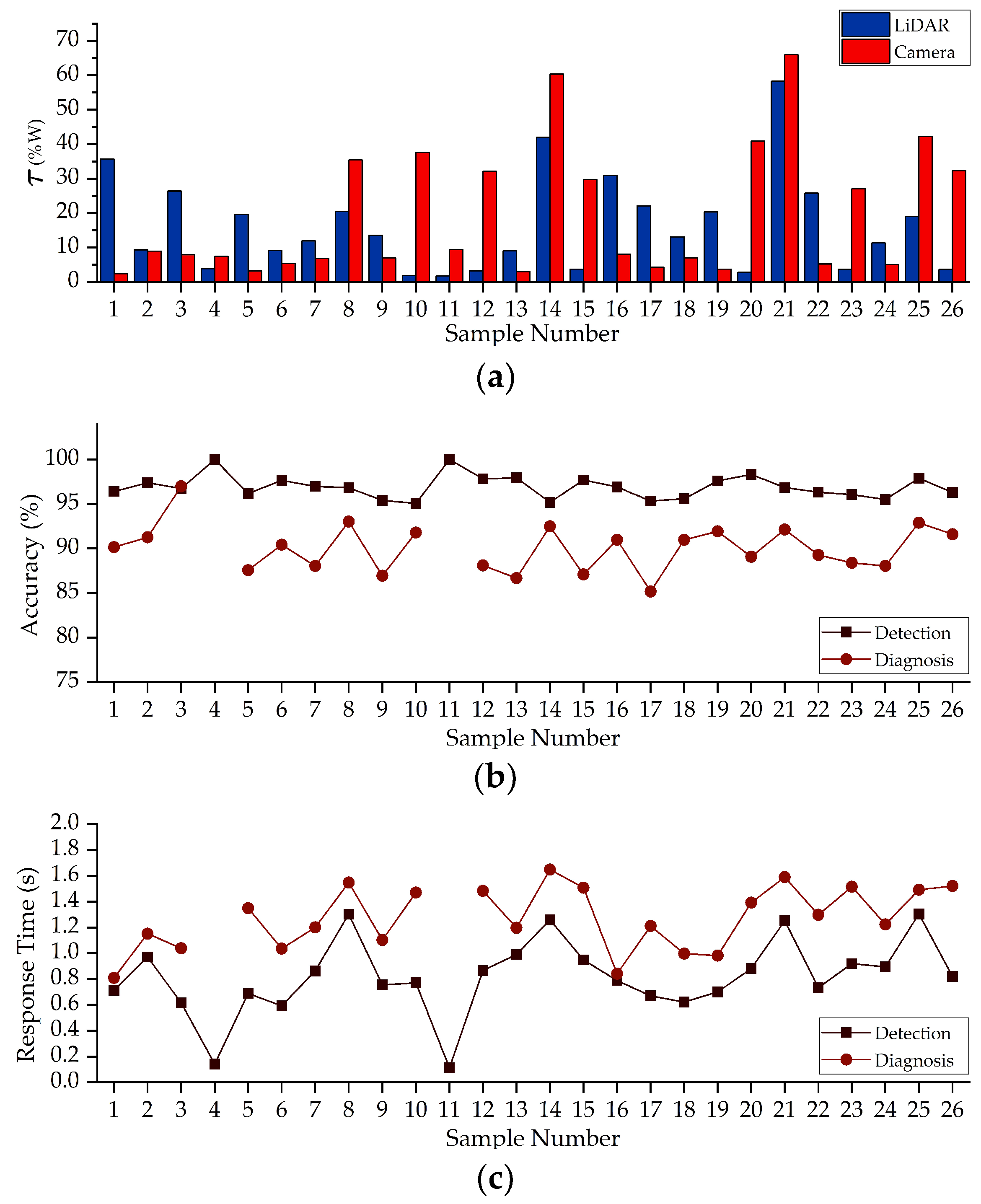
Based on the established criteria for positioning error relative to the “ground truth”, the accuracy of fault detection averages 96.93%. No false positives occurred in scenarios without injected faults. Therefore, even in the presence of algorithmic delays in real-world vehicle deployment, the hardware-redundant fault detection method is commendable and applicable to autonomous driving sensor systems;

(2)

The fault diagnoser exhibited no misjudgments during testing. To observe differences in various fault types, we focused on the SoftMax output probabilities of the CNN, as outlined in Section 2.4.4. Notably, the accuracy for individual faults for LiDAR and the camera was comparable (89.67% and 89.42%, respectively). When misalignment faults occurred simultaneously in LiDAR and the camera, there was an improvement in diagnostic accuracy of approximately 3.6%, reaching 92.73%;

(3)

Regarding response times, the fault detector exhibited an average response time of 0.13 s in no-fault scenarios. For isolated LiDAR faults, the response time (averaging 0.76 s) was faster than isolated camera faults (averaging 0.87 s). In cases of misalignment faults occurring in both LiDAR and the camera, the response time was the longest, reaching an average of 1.28 s. A similar trend was observed in the fault diagnoser. The response time for isolated LiDAR faults (averaging 1.10 s) was faster than isolated camera faults (averaging 1.48 s), while misalignment faults in both resulted in the longest response time, averaging 1.57 s. Overall, fault diagnosis exhibited longer response times compared to fault detection, attributed to the CNN’s need for a time series of samples rather than a single-frame data approach used in fault detection.

3.2. Validation on Real-World Vehicle

In the experiments conducted on the actual vehicle, to facilitate comparison, we employed identical experimental conditions and statistical methods as outlined in Section 3.1. The results are presented in Figure 17 and Table 3.

Figure 17. Results of the real-world vehicle from 26 experiment segments are extracted, and the meanings of subfigures (a–c) remain consistent in Figure 15.

Table 3. Statistics on the results of the validation of the real-world vehicle.

Results		Values
Average fault detection accuracy		95.33%
Average fault diagnosis accuracy	Corruptions (L)	82.23%
	Corruptions (C)	81.46%
	Misalignment	87.31%
Average fault detection response time	No Fault	0.13 s
	Corruptions (L)	0.82 s
	Corruptions (C)	0.92 s
	Misalignment	1.36 s
Average fault diagnosis response time	Corruptions (L)	1.18 s
	Corruptions (C)	1.56 s
	Misalignment	1.66 s

The validation results from the real-world vehicle experiments exhibit similar trends to those obtained with the dataset. The proposed fault detection method achieves an average detection accuracy of 95.33% for real vehicles. In scenarios without faults, there are no false positives. However, it is noted that the detector exhibits a longer (on average, increased by 7.40%) response time. Although there is a decrease in the accuracy of fault diagnosis (on average, reduced by 8.02%), it remains above 80% overall. The response time for fault diagnosis is also longer (on average, increased by 6.25%). It is evident that the proposed fault diagnosis method remains effective and efficient in real-world vehicle experiments, despite a reduction in performance. The performance decline can be attributed to the simultaneous execution of decision-making and control tasks on the control computer of the autonomous vehicle. Additionally, differences in sensor arrangement and environmental conditions, as compared to the nuScenes dataset, contribute to the reduced performance in real-world fault diagnosis.

4. Discussion and Conclusions

This study introduces a fault diagnosis method for autonomous driving sensing systems using a combination of hardware redundancy and analytical redundancy. Initially, we define 12 common faults present in LiDAR and cameras, simulating these faults by extending the nuScenes dataset. Subsequently, we employ heterogeneous hardware redundancy, leveraging MMW radar cluster targets as a basis for the real-time analysis of the Euclidean distance between the identified target centers from LiDAR- and camera-collected data for fault detection. Thirdly, we introduce information complexity to evaluate the fluctuation of transmitted information in the event of sensing system faults. Using 3D and 2D temporal entropy as fault analysis metrics for LiDAR and cameras, we construct a CNN-based temporal data feature recognition and classification neural network as a fault diagnoser. Experimental results demonstrate the accuracy of our proposed fault diagnosis method on both the dataset’s validation set and a real vehicle. The accuracy of fault detection averages 96.93% on the validation set and 95.33% in real vehicle experiments, with no false positives in scenarios without faults. Additionally, the fault diagnosis accuracy averages 90.12% on the validation set and 82.89% in real vehicle experiments. Simultaneously, the system exhibits rapid response times, with fault detection response times averaging 0.81 s on the validation set and 0.87 s in real vehicle experiments. This suggests that the system can accurately detect faults and determine their severity within these response times, notifying the system whether functional degradation is required. The fault diagnosis response times average 1.28 s on the validation set and 1.36 s in real vehicle experiments, enabling the system to identify the source and type of faults within this timeframe for subsequent inspection and repair.

Our study proposes an effective fault diagnosis method for the autonomous driving sensing systems, but there are several limitations worth further exploration in future research: (1) It is necessary to establish a more comprehensive and richer dataset dedicated to fault diagnosis to develop more accurate and efficient diagnostic methods. (2) In real-world autonomous driving deployments, a more diverse range of sensors is employed, including infrared sensors, event cameras, etc. Therefore, it is essential to develop more universal and unified fault diagnosis methods. (3) Further validation and development should be conducted on microcontrollers or platforms dedicated to autonomous driving to ensure applicability in real-world autonomous driving scenarios. (4) Even the most stable sensors cannot guarantee fault- and error-free operation under all weather conditions. During the hardware redundancy phase, it is crucial to consider more redundancy methods among sensors. (5) The inherent drawbacks and discontinuities of the MMW radar need to be taken into consideration to enhance the overall accuracy and latency conditions.

References

- Hou, W.; Li, W.; Li, P. Fault diagnosis of the autonomous driving perception system based on information fusion. Sensors 2023, 23, 5110. [Google Scholar] [CrossRef] [PubMed]
- Zhang, Y.; He, L.; Cheng, G. MLPC-CNN: A Multi-Sensor Vibration Signal Fault Diagnosis Method under Less Computing Resources. Measurement 2022, 188, 110407. [Google Scholar] [CrossRef]
- Zhao, G.; Li, J.; Ma, L. Design and implementation of vehicle trajectory perception with multi-sensor information fusion. Electron. Des. Eng. 2022, 1, 1–7. [Google Scholar]
- Gao, Z.; Cecati, C.; Ding, S.X. A survey of fault diagnosis and fault-tolerant techniques—Part I: Fault diagnosis with model-based and signal-based approaches. IEEE Trans. Ind. Electron. 2015, 62, 3757–3767. [Google Scholar] [CrossRef]
- Gao, Z.; Cecati, C.; Ding, S.X. A survey of fault diagnosis and fault-tolerant techniques—Part II: Fault diagnosis with knowledge-based and hybrid/active approaches. IEEE Trans. Ind. Electron. 2015, 62, 3768–3774. [Google Scholar] [CrossRef]
- Willsky, A.S. A survey of design methods for failure detection in dynamic systems. Automatica 1976, 12, 601–611. [Google Scholar] [CrossRef]
- Van Wyk, F.; Wang, Y.; Khojandi, A.; Masoud, N. Real-time sensor anomaly detection and identification in automated vehicles. IEEE Trans. Intell. Transp. Syst. 2019, 21, 1264–1276. [Google Scholar] [CrossRef]
- Muenchhof, M.; Isermann, R. Comparison of change detection methods for a residual of a hydraulic servo-axis. IFAC Proc. Vol. 2005, 38, 317–322. [Google Scholar] [CrossRef]
- Chan, C.W.; Hua, S.; Hong-Yue, Z. Application of fully decoupled parity equation in fault detection and identification of DC motors. IEEE Trans. Ind. Electron. 2006, 53, 1277–1284. [Google Scholar] [CrossRef]
- Escobet, T.; Travé-Massuyès, L. Parameter Estimation Methods for Fault Detection and Isolation. Bridge Workshop Notes. 2001, pp. 1–11. Available online: https://homepages.laas.fr/louise/Papiers/Escobet%20&%20Trave-Massuyes%202001.pdf (accessed on 11 November 2023).
- Hilbert, M.; Kuch, C.; Nienhaus, K. Observer based condition monitoring of the generator temperature integrated in the wind turbine controller. In Proceedings of the EWEA 2013 Scientific Proceedings, Vienna, Austria, 4–7 February 2013; pp. 189–193. [Google Scholar]
- Heredia, G.; Ollero, A. Sensor fault detection in small autonomous helicopters using observer/Kalman filter identification. In Proceedings of the 2009 IEEE International Conference on Mechatronics, Malaga, Spain, 14–17 April 2009; pp. 1–6. [Google Scholar]
- Wang, J.; Zhang, Y.; Cen, G. Fault diagnosis method of hydraulic condition monitoring system based on information entropy. Comput. Eng. Des. 2021, 8, 2257–2264. [Google Scholar]
- Chandola, V.; Banerjee, A.; Kumar, V. Anomaly detection: A survey. ACM Comput. Surv. (CSUR) 2009, 41, 1–58. [Google Scholar] [CrossRef]
- Sharifi, R.; Langari, R. Nonlinear Sensor Fault Diagnosis Using Mixture of Probabilistic PCA Models. Mech. Syst. Signal Process. 2017, 85, 638–650. [Google Scholar] [CrossRef]
- Yin, S.; Ding, S.X.; Xie, X.; Luo, H. A review on basic data-driven approaches for industrial process monitoring. IEEE Trans. Ind. Electron. 2014, 61, 6418–6428. [Google Scholar] [CrossRef]
- Meskin, N.; Khorasani, K. Fault Detection and Isolation: Multi-Vehicle Unmanned Systems; Springer Science & Business Media: Berlin, Germany, 2011. [Google Scholar]
- Li, M.; Wang, Y.-X.; Ramanan, D. Towards streaming perception. In Proceedings of the Computer Vision–ECCV 2020: 16th European Conference, Glasgow, UK, 23–28 August 2020; Proceedings, Part II 16. pp. 473–488. [Google Scholar]
- Dong, Y.; Kang, C.; Zhang, J.; Zhu, Z.; Wang, Y.; Yang, X.; Su, H.; Wei, X.; Zhu, J. Benchmarking Robustness of 3D Object Detection to Common Corruptions. In Proceedings of the IEEE/CVF Conference on Computer Vision and Pattern Recognition, Vancouver, BC, Canada, 17–24 June 2023; pp. 1022–1032. [Google Scholar]
- Ferracuti, F.; Giantomassi, A.; Ippoliti, G.; Longhi, S. Multi-Scale PCA based fault diagnosis for rotating electrical machines. In Proceedings of the 8th ACD 2010 European Workshop on Advanced Control and Diagnosis Department of Engineering, Ferrara, Italy, 18–19 November 2010; pp. 296–301. [Google Scholar]
- Yu, K.; Tao, T.; Xie, H.; Lin, Z.; Liang, T.; Wang, B.; Chen, P.; Hao, D.; Wang, Y.; Liang, X. Benchmarking the robustness of lidar-camera fusion for 3d object detection. In Proceedings of the IEEE/CVF Conference on Computer Vision and Pattern Recognition, Vancouver, BC, Canada, 18–22 June 2023; pp. 3187–3197. [Google Scholar]
- Realpe, M.; Vintimilla, B.X.; Vlacic, L. A Fault Tolerant Perception System for Autonomous Vehicles. In Proceedings of the 2016 35th Chinese Control Conference (CCC), Chengdu, China, 27–29 July 2016; pp. 6531–6536. [Google Scholar]
- Schlager, B.; Goelles, T.; Behmer, M.; Muckenhuber, S.; Payer, J.; Watzenig, D. Automotive lidar and vibration: Resonance, inertial measurement unit, and effects on the point cloud. IEEE Open J. Intell. Transp. Syst. 2022, 3, 426–434. [Google Scholar] [CrossRef]
- Hendrycks, D.; Dietterich, T. Benchmarking neural network robustness to common corruptions and perturbations. arXiv 2019, arXiv:1903.12261. [Google Scholar]
- Li, Z.; Wang, W.; Li, H.; Xie, E.; Sima, C.; Lu, T.; Qiao, Y.; Dai, J. Bevformer: Learning bird’s-eye-view representation from multi-camera images via spatiotemporal transformers. In Proceedings of the European Conference on Computer Vision, Tel Aviv, Israel, 23–27 October 2022; pp. 1–18. [Google Scholar]
- Berger, M.; Tagliasacchi, A.; Seversky, L.M.; Alliez, P.; Levine, J.A.; Sharf, A.; Silva, C.T. State of the art in surface reconstruction from point clouds. In Proceedings of the 35th Annual Conference of the European Association for Computer Graphics, Eurographics 2014-State of the Art Reports, Strasbourg, France, 7–11 April 2014. [Google Scholar]
- Carballo, A.; Lambert, J.; Monrroy, A.; Wong, D.; Narksri, P.; Kitsukawa, Y.; Takeuchi, E.; Kato, S.; Takeda, K. LIBRE: The multiple 3D LiDAR dataset. In Proceedings of the 2020 IEEE Intelligent Vehicles Symposium (IV), Las Vegas, NV, USA, 19 October–13 November 2020; pp. 1094–1101. [Google Scholar]
- Li, X.; Chen, Y.; Zhu, Y.; Wang, S.; Zhang, R.; Xue, H. ImageNet-E: Benchmarking Neural Network Robustness via Attribute Editing. In Proceedings of the IEEE/CVF Conference on Computer Vision and Pattern Recognition, Vancouver, BC, Canada, 18–22 June 2023; pp. 20371–20381. [Google Scholar]
- Ren, J.; Pan, L.; Liu, Z. Benchmarking and analyzing point cloud classification under corruptions. In Proceedings of the International Conference on Machine Learning, Baltimore, MD, USA, 17–23 July 2022; pp. 18559–18575. [Google Scholar]
- Geiger, A.; Lenz, P.; Urtasun, R. Are we ready for autonomous driving? the kitti vision benchmark suite. In Proceedings of the 2012 IEEE Conference on Computer Vision and Pattern Recognition, Providence, RI, USA, 16–21 June 2012; pp. 3354–3361. [Google Scholar]
- Briñón-Arranz, L.; Rakotovao, T.; Creuzet, T.; Karaoguz, C.; El-Hamzaoui, O. A methodology for analyzing the impact of crosstalk on LIDAR measurements. In Proceedings of the 2021 IEEE Sensors, Sydney, Australia, 31 October–3 November 2021; pp. 1–4. [Google Scholar]
- Li, S.; Wang, Z.; Juefei-Xu, F.; Guo, Q.; Li, X.; Ma, L. Common corruption robustness of point cloud detectors: Benchmark and enhancement. IEEE Trans. Multimed. 2023, 1–12. [Google Scholar] [CrossRef]
- Mao, J.; Niu, M.; Jiang, C.; Chen, J.; Liang, X.; Li, Y.; Ye, C.; Zhang, W.; Li, Z.; Yu, J. One Million Scenes for Autonomous Driving: ONCE Dataset. In Proceedings of the Thirty-fifth Conference on Neural Information Processing Systems Datasets and Benchmarks Track (Round 1), Online, 7–10 December 2021. [Google Scholar]
- Caesar, H.; Bankiti, V.; Lang, A.H.; Vora, S.; Liong, V.E.; Xu, Q.; Krishnan, A.; Pan, Y.; Baldan, G.; Beijbom, O. nuscenes: A multimodal dataset for autonomous driving. In Proceedings of the IEEE/CVF Conference on Computer Vision and Pattern Recognition, Seattle, WA, USA, 14–19 June 2020; pp. 11621–11631. [Google Scholar]
- Jung, A. Imgaug documentation. Readthedocs. Io Jun 2019, 25. Available online: https://media.readthedocs.org/pdf/imgaug/stable/imgaug.pdf (accessed on 15 November 2023).
- Fan, Z.; Wang, S.; Pu, X.; Wei, H.; Liu, Y.; Sui, X.; Chen, Q. Fusion-Former: Fusion Features across Transformer and Convolution for Building Change Detection. Electronics 2023, 12, 4823. [Google Scholar] [CrossRef]
- Guo, J.; Han, K.; Wu, H.; Tang, Y.; Chen, X.; Wang, Y.; Xu, C. Cmt: Convolutional neural networks meet vision transformers. In Proceedings of the IEEE/CVF Conference on Computer Vision and Pattern Recognition, New Orleans, LA, USA, 18–24 June 2022; pp. 12175–12185. [Google Scholar]
- Liu, Z.; Tang, H.; Amini, A.; Yang, X.; Mao, H.; Rus, D.L.; Han, S. Bevfusion: Multi-task multi-sensor fusion with unified bird’s-eye view representation. In Proceedings of the 2023 IEEE International Conference on Robotics and Automation (ICRA), Singapore, 17–19 November 2023; pp. 2774–2781. [Google Scholar]
- Schubert, E.; Sander, J.; Ester, M.; Kriegel, H.P.; Xu, X. DBSCAN revisited, revisited: Why and how you should (still) use DBSCAN. ACM Trans. Database Syst. (TODS) 2017, 42, 1–21. [Google Scholar] [CrossRef]
- Lu, W.; Zhou, Y.; Wan, G.; Hou, S.; Song, S. L3-net: Towards learning based lidar localization for autonomous driving. In Proceedings of the IEEE/CVF Conference on Computer Vision and Pattern Recognition, Long Beach, CA, USA, 15–20 June 2019; pp. 6389–6398. [Google Scholar]
- Wang, C.-Y.; Bochkovskiy, A.; Liao, H.-Y.M. YOLOv7: Trainable bag-of-freebies sets new state-of-the-art for real-time object detectors. In Proceedings of the IEEE/CVF Conference on Computer Vision and Pattern Recognition, Vancouver, BC, Canada, 18–22 June 2023; pp. 7464–7475. [Google Scholar]
- Huang, H.; Huang, X.; Ding, W.; Yang, M.; Yu, X.; Pang, J. Vehicle vibro-acoustical comfort optimization using a multi-objective interval analysis method. Expert Syst. Appl. 2023, 213, 119001. [Google Scholar] [CrossRef]
- Tan, F.; Liu, W.; Huang, L.; Zhai, C. Object Re-Identification Algorithm Based on Weighted Euclidean Distance Metric. J. South China Univ. Technol. Nat. Sci. Ed. 2015, 9, 88–94. [Google Scholar]
- Wang, X.; Zhu, Z.; Zhang, Y.; Huang, G.; Ye, Y.; Xu, W.; Chen, Z.; Wang, X. Are We Ready for Vision-Centric Driving Streaming Perception? The ASAP Benchmark. In Proceedings of the IEEE/CVF Conference on Computer Vision and Pattern Recognition, Vancouver, BC, Canada, 18–22 June 2023; pp. 9600–9610. [Google Scholar]
- Rao, M.; Chen, Y.; Vemuri, B.C.; Wang, F. Cumulative residual entropy: A new measure of information. IEEE Trans. Inf. Theory 2004, 50, 1220–1228. [Google Scholar] [CrossRef]
- Huang, H.; Lim, T.C.; Wu, J.; Ding, W.; Pang, J. Multitarget prediction and optimization of pure electric vehicle tire/road airborne noise sound quality based on a knowledge-and data-driven method. Mech. Syst. Signal Process. 2023, 197, 110361. [Google Scholar] [CrossRef]
- Huang, H.; Huang, X.; Ding, W.; Zhang, S.; Pang, J. Optimization of electric vehicle sound package based on LSTM with an adaptive learning rate forest and multiple-level multiple-object method. Mech. Syst. Signal Process. 2023, 187, 109932. [Google Scholar] [CrossRef]
Disclaimer/Publisher’s Note: The statements, opinions and data contained in all publications are solely those of the individual author(s) and contributor(s) and not of MDPI and/or the editor(s). MDPI and/or the editor(s) disclaim responsibility for any injury to people or property resulting from any ideas, methods, instructions or products referred to in the content. |
© 2024 by the authors. Licensee MDPI, Basel, Switzerland. This article is an open access article distributed under the terms and conditions of the Creative Commons Attribution (CC BY) license (https://creativecommons.org/licenses/by/4.0/).