GaitMGL: Multi-Scale Temporal Dimension and Global–Local Feature Fusion for Gait Recognition

Abstract

Gait recognition has received widespread attention due to its non-intrusive recognition mechanism. Currently, most gait recognition methods use appearance-based recognition methods, and such methods are easily affected by occlusions when facing complex environments, which in turn affects the recognition accuracy. With the maturity of pose estimation techniques, model-based gait recognition methods have received more and more attention due to their robustness in complex environments. However, the current model-based gait recognition methods mainly focus on modeling the global feature information in the spatial dimension, ignoring the importance of local features and their influence on recognition accuracy. Meanwhile, in the temporal dimension, these methods usually use single-scale temporal information extraction, which does not take into account the inconsistency of the motion cycles of the limbs when a human body is walking (e.g., arm swing and leg pace), leading to the loss of some limb temporal information. To solve these problems, we propose a gait recognition network based on a Global–Local Graph Convolutional Network, called GaitMGL. Specifically, we introduce a new spatio-temporal feature extraction module, MGL (Multi-scale Temporal and Global–Local Spatial Extraction Module), which consists of GLGCN (Global–Local Graph Convolutional Network) and MTCN (Multi-scale Temporal Convolutional Network). GLGCN models both global and local features, and extracts global–local motion information. MTCN, on the other hand, takes into account the inconsistency of local limb motion cycles, and facilitates multi-scale temporal convolution to capture the temporal information of limb motion. In short, our GaitMGL solves the problems of loss of local information and loss of temporal information at a single scale that exist in existing model-based gait recognition networks. We evaluated our method on three publicly available datasets, CASIA-B, Gait3D, and GREW, and the experimental results show that our method demonstrates surprising performance and achieves an accuracy of 63.12% in the dataset GREW, exceeding all existing model-based gait recognition networks.

1. Introduction

Gait [1,2] serves as a characteristic that is difficult to hide when persons walk. Compared with facial recognition [3] and fingerprint recognition [4], gait recognition can recognize an observed person from a distance and does not require the cooperation of the observed person. Because of its characteristics, gait recognition has a wide range of application scenarios and great research value in security, criminal investigation, and other fields. In real scenarios, human gait is affected by many aspects, such as carrying objects, bloated coats, and changes in camera viewpoints, which all bring significant challenges to computer recognition.

With the development of deep learning [5,6,7,8,9,10,11,12,13], researchers have begun to introduce deep learning methods to solve these problems and have achieved good results [14,15,16,17,18,19,20,21,22,23,24,25,26,27,28,29,30,31]. Existing gait recognition networks can be approximately divided into two categories based on the type of input data: silhouette-based gait recognition networks [14,15,16,17,18,19,20,21] and human model-based gait recognition networks [22,23,24,25,26,27,28,29,30].

A silhouette-based gait recognition network is a recognition method that extracts human gait motion features using contour plots as inputs. For example, Gaitset [14] considered a set of contour plot sequences as a whole and extracted gait features by directly pooling time series. GaitPart [15] proposes that various parts of human gait have distinctly different morphologies and movement patterns, and started to model the human body locally as well as in the time dimension. GaitGL [16] not only focuses on the relationship between human body localities, but also emphasizes the relationship between localities. All these approaches have achieved good performance in the uncovered situations. However, they lack robustness in complex environments where occlusion exists. Model-based gait recognition methods, on the other hand, show strong robustness in this regard.

The model-based gait recognition network captures the motion characteristics of the human body while walking using human joint point information as input. With the maturity of pose estimation techniques, model-based gait recognition methods have received increasing attention. PoseGait [22] takes manually computed 3D skeletal data as input and utilizes convolutional neural networks (CNNs) to capture spatio-temporal features of a person as they walk, thereby eliminating the effects generated by occlusion. GaitGraph [23] takes the a priori matrix A and the skeletal data as inputs and obtains their spatio-temporal features for identification. Due to the limited information of the skeleton, GaitGraph2 [24] computes the limited skeleton information to obtain more dimensional information (relative positions of joints, joint velocities, and bone angles), and then adopts the multi-branching input, which makes the performance of GaitGraph2 improve tremendously. Nonetheless, it still falls short of the current state-of-the-art appearance-based networks. As with earlier appearance-based gait recognition networks, existing skeleton-based methods suffer from two problems. First, in the spatial dimension, they are limited to obtaining global skeleton information and lack attention to local information about the human body. Second, in the temporal dimension, it lacks the flexibility of graph convolutional networks to process the temporal dimension, and adopts a fixed scale to obtain temporal information, ignoring the fact that the human body does not have the same motion period of each limb part in a gait cycle. This leads to the problem of localized loss of temporal information when extracting temporal information.

To address these issues, this paper proposes a new gait recognition framework, GaitMGL. GaitMGL is built on top of a new Multi-scale Temporal and Global–Local Graph Convolutional Module, MGL (Multi-scale temporal and global–local spatial extraction modules), which consists of two parts: MTCN (Multi-scale Temporal Convolutional Network) and GLGCN (Global–Local Graph Convolutional Network). In the time dimension, due to the different motion cycles of each body part during human walking, as shown in Figure 1, the leg is still in the first cycle when the upper limb arm completes the first cycle of motion. It can be seen that the cycles of arm swing and walking rhythm are not the same. The use of a single fixed-scale convolution results in the loss of temporal information for some body parts. Multi-scale convolution in MTCN utilizes multiple convolution modules to extract temporal features of different lengths to avoid the loss of temporal information. In the spatial dimension, GLGCN utilizes skeleton global and local information to obtain better feature representation. As shown in Figure 1, during human walking, each body part has its unique expression, such as the swing of the upper limbs and the rhythm of the lower limbs’ stride. Since the skeleton only retains the necessary information, more expressive movements are performed by the arms and legs, and other parts provide less motion information; the arms and legs basically include all the local motion information. While the motion information expressed by body parts other than the arms and legs (such as the head and torso) is limited, in order to prevent the loss of motion information, we consider these parts collectively with the arms, thus treating them as the upper limb skeleton in this paper. Based on this, our GLGCN divides the skeleton into upper limb skeleton (including arms, head, and body) and lower limb skeleton (including legs), as shown in Figure 2, and models each part separately to obtain more local information, and at the same time extracts the feature information of the whole skeleton to generate the feature representation with global and local information.

The primary contributions of this study are succinctly summarized as follows:

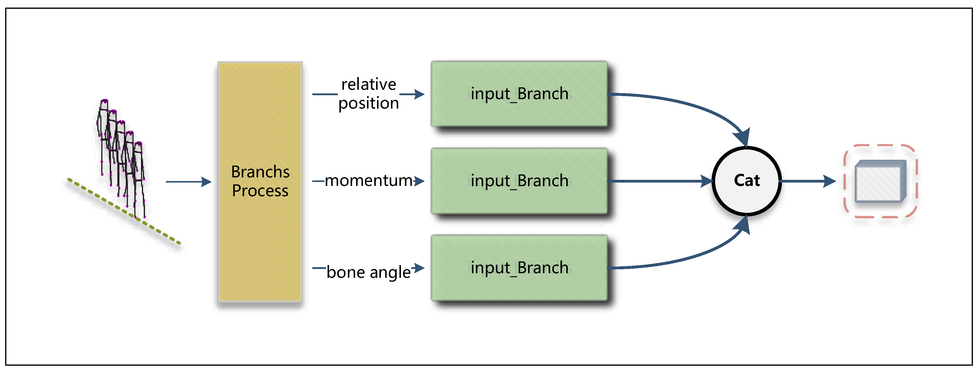
• We introduce the novel GaitMGL network model, designed to efficiently extract crucial global and local features from skeleton sequences.
• We propose a novel temporal extraction module called MTCN, which is suitable for temporal extraction at various scales, enhances the flexibility of extracting temporal information from model-based gait recognition networks, and improves the whole effect of temporal feature extraction.
• Our GaitMGL network is thoroughly assessed on publicly available datasets including CASIA-B, Gait3D, and GREW. The experimental data clearly indicate that GaitMGL outperforms state-of-the-art (SOTA) skeletal gait recognition models. In particular, on the GREW dataset, the accuracy of our model reaches an impressive 63.12%, nearly 30% higher than the best existing model-based gait recognition network. This performance improvement makes model-based gait recognition more competitive in the field.

These contributions emphasize the importance and potential of GaitMGL as a new gait recognition framework that is expected to enhance the competitiveness of skeleton-based gait recognition networks.

2. Related Work

Different from the type of input data, deep learning-based gait recognition networks can be approximately categorized into two groups: silhouette-based gait recognition networks and model-based gait recognition networks. This section describes each of these two types of methods based on the input data type.

2.1. Silhouette-Based Gait Recognition Networks

Silhouette-based gait recognition networks have long been a mainstay in the realm of gait recognition. In its initial stages, researchers compress the entire sequence into individual images, such as gait energy images (GEIs). These images are then subjected to a convolutional neural network (CNN) to capture gait features. For example, Shiraga et al. [32] proposed the GEINET network to extract features for GEI. However, this approach leads to the loss of critical spatio-temporal information inherent in the original silhouette images. Subsequently, many methods are beginning to extract gait features from raw silhouette maps. Chao et al. [14] proposed Gaitset, which extracts spatio-temporal features by treating gait sequences as unordered sets. The method showed significant robustness on various datasets. Fan et al. observed that different parts of the human body have different movement patterns during walking, and for the first time, used the concept of localization for gait recognition and proposed a part-based gait recognition network, GaitPart [15], which captures the spatio-temporal information of local features by modeling them. Recognizing the lack of connection between local features of gait and global features, Lin et al. proposed GaitGL [16], a gait recognition model that fuses global local features; GaitGL [16] transforms global gait features into local gait features by means of masking and learns the relationship between them, so that the global and local letters are fused, and the connection between localities is also enhanced. Huang et al. pointed out that a fixed-size local information extraction window is not applicable to each part of the human body (each part of the human body has different lengths and thicknesses), and proposed 3DLocal [17], which can adaptively adjust the size of the local window, making the gait recognition more flexible in extracting local information about the human body. GaitEdge [18] designed a learnable intermediate modality for building end-to-end gait recognition models. Currently, contour-based gait recognition methods exhibit superior performance to model-based gait recognition methods. However, while providing high performance, they also impose significant computational and storage burdens. Model-based gait recognition methods provide solutions to these problems. In addition, they exhibit greater robustness on non-laboratory datasets.

2.2. Model-Based Gait Recognition Networks

Model-based gait recognition networks primarily rely on skeleton data as their input source. In the early stages, skeleton data extraction depended on manually devised formulas or rules applied to RGB images. PoseGait [22] was a pioneering attempt in the gait domain to utilize manually engineered features from 3D pose estimation. It computed joint angles, bone lengths, and joint movements using 3D keypoints in Euclidean space. These manually engineered features were fed as inputs, allowing CNNs to learn their spatio-temporal characteristics. However, this approach proved cumbersome and lacked accuracy, placing constraints on the development of model-based methods.

With the maturity of pose estimation techniques [33,34,35], model-based methods have come back into focus. GaitGraph [23] pioneered the integration of Graph Convolutional Network (GCN) architecture with model-based gait recognition methods. GaitGraph [23] captures the spatio-temporal dependence of gait features by modeling the spatial location of each time step and spatial position, and using graph convolution and convolution operations to extract features from the spatial position information of the joints around it, as well as from its own position information at adjacent times. GaitGraph [23] significantly improved the performance of model-based gait recognition methods. The second year GaitGraph2 [24] builds on GaitGraph [23] by introducing residual connectivity and feature dimensionality reduction bottleneck structure. Meanwhile, GaitGraph2 [24] also adopts high-order inputs with multiple branches, which enhances the competitiveness of model-based methods in gait recognition.

Nonetheless, it still falls short of the current SOTA appearance-based networks. Similar to the early appearance-based methods, the existing model-based methods only extract global spatial information, ignoring the effect of local features on the gait recognition results in terms of extracting spatio-temporal information, and in terms of temporal aspects, the extraction of temporal features at a single scale can easily lead to the problem of loss of temporal information, all of which limit the performance of model-based gait recognition methods. Taking inspiration from the evolution of appearance-based methods, we are transitioning from capturing global features to including global and local features. In addition, we likewise utilize the idea of global localization in space to capture the temporal information of the motion of different parts of the human body during a gait cycle, which solves the problem of losing temporal information caused by single-scale temporal extraction.

3. Proposed Method

In this section, we explain our proposed backbone network in detail. This backbone is designed to capture advanced spatio-temporal features from gait sequences. Additionally, we will introduce some key modules, including the Global–Local Spatial Graph Convolutional Network (GLGCN) and the Multi-Scale Temporal Convolutional Network (MTCN).

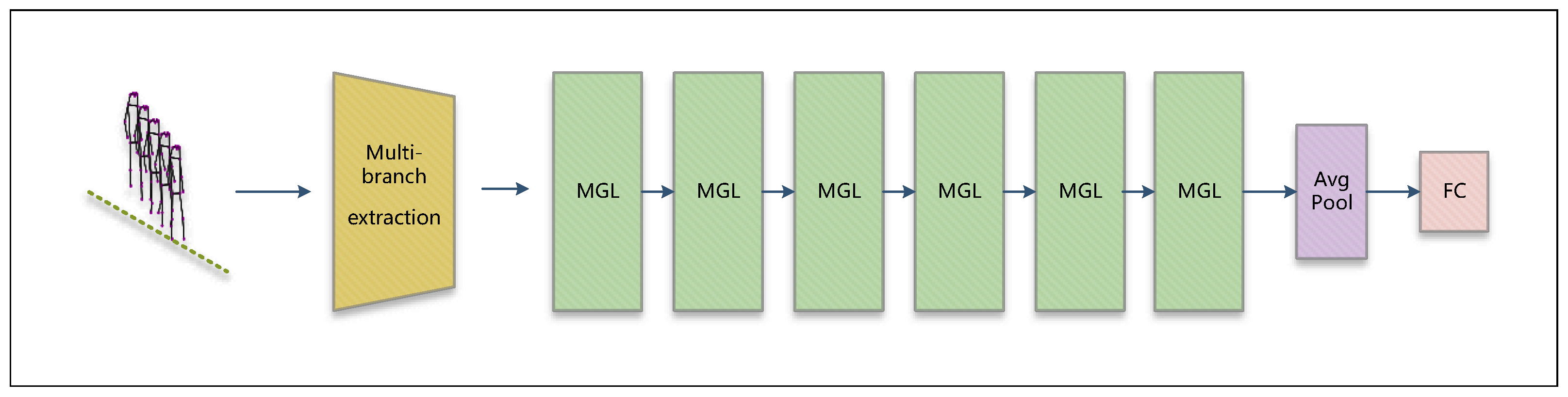
3.1. Overall Architecture

The general framework of GaitMGL is shown in Figure 3. The input gait sequence goes through the branch extraction module to extract multi-branch features and generate gait primary features containing multi-branch features. Then the spatio-temporal features are extracted by multiple MGL modules to generate the advanced gait features. Finally, the advanced gait features are average pooled and mapped to generate discriminative features. During the training process, a triplet loss function is used to train the model.

The framework of our multi-branch extraction module is shown in Figure 4. The multi-branch extraction module includes multi-branch processing and three input branch extraction modules. Among them, the multi-branch processing converts the input gait skeleton sequence computation into joint point relative position information streams, joint momentum streams, and bone angle streams. Each information stream is passed to a different input branch extraction module to extract feature information, and the final extracted feature information is channel spliced. It is worth mentioning that the input branch extraction module is a combination of three MGL modules. The whole multi-branch extraction module can be represented as follows:

$$X_{out}=Concat(F\left(\alpha \left(X_{in}\right)\right),F\left(\beta \left(X_{in}\right)\right),F\left(\theta \left(X_{in}\right)\right))$$

(1)

where $X_{in}$, $X_{out}$ represent the input and output. $\alpha$(·), $\beta$(·), and $\theta$(·) correspond to different stream processing streams (joint relative position stream, joint momentum stream, skeletal bone angle stream). F(·) is the feature extraction by the input branch on the input stream, and $Concat$ represents the channel-wise concatenation operation.

The primary gait features generated by the branch extraction module are passed to a series of MGL modules for extracting their spatio-temporal features. The process of extracting spatio-temporal features through MGL modules is shown in Figure 5. First, the primary gait feature is processed by GLGCN (Global–Local Graph Convolutional Network) in MGL in order to extract the global–local information and generate new gait information with global–local features. Then, it is passed to MTCN (Multi-scale Spatio-temporal Convolutional Network), which captures the spatio-temporal gait feature information at different scales using convolution kernels of different sizes. Finally, the captured spatio-temporal information is output. This process can be represented by the following equation:

$$X_{out}=F_T\left(F_{GL}\left(X_{in}\right)\right)$$

(2)

where $X_{in}$ and $X_{out}$ stand for the input and output, respectively. $F_T$(·) represents the extraction of temporal features by MTCN, and $F_{GL}$(·) represents the extraction of spatial features from the data.

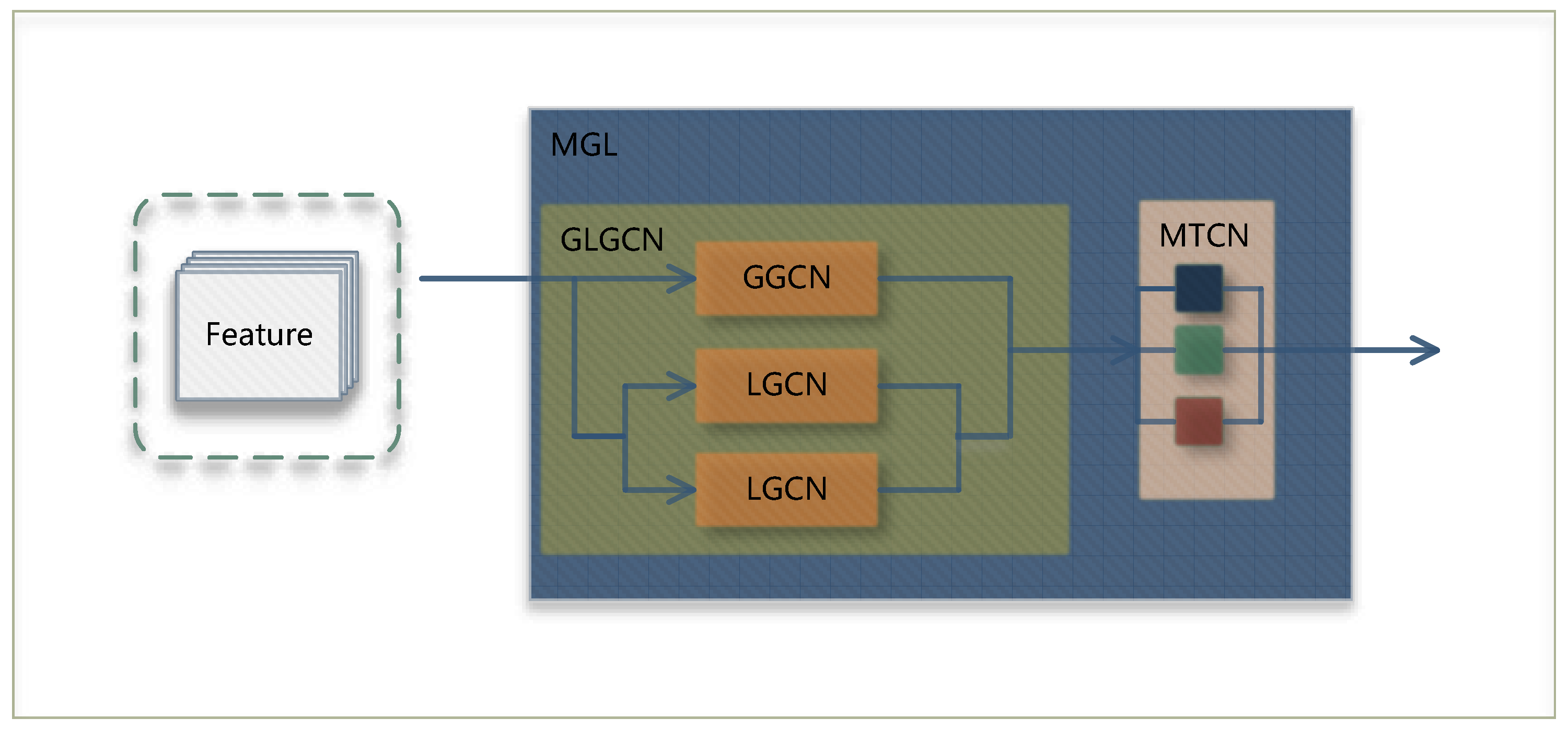
3.2. Global–Local Graph Convolutional Network

Despite the excellent performance achieved by previous gait graph convolutional networks [23,24] in recognition, they have always been limited by their neglect of local information, which has restricted their accuracy. Their focus on global information extraction makes it difficult for them to pay attention to the loss of local information, resulting in the omission of local details. However, local information is crucial for gait analysis.

To solve this problem, we propose a new graph space extraction network, GLGCN, to fully extract global and local information. GLGCN extracts the global spatial features of the gait features using global graph convolution network (GGCN), and at the same time, divides the gait features and a priori matrices A along the joint dimension into upper limb gait features and upper limb a priori matrices $A^{up}$ (containing only the upper limb joints), as well as lower limb gait features and a priori matrices $A^{low}$ (containing only the lower limb joints). Then its local feature information is extracted using Local Graph Convolutional Network (LGCN), and then the obtained local information is spliced along the articulation point dimension to obtain new local feature information. Finally, it is summed with the global features to generate global–local gait feature information, and finally output after normalization. The specific processing of GLGCN is illustrated in Figure 6, as shown. This process can be mathematically formalized as follows:

$$X_{out}=Concat(F_{Lconv}\left(X_{in}^{up}\right),F_{Lconv}\left(X_{in}^{low}\right))+F_{Gconv}\left(X_{in}\right)$$

(3)

where $X_{in}$, $X_{out}$, $X_{in}^{up}$, and $X_{in}^{low}$, respectively, represent the input, output, upper limb part of $X_{in}$, and lower limb part of $X_{in}$. $Concat$ represents operations of channel concatenation, and + denotes an element-by-element addition operation.

GLGCN effectively extracts local information from both upper and lower limbs. By concatenating this information, it enhances the connections between local features, resulting in new local-to-local features. These features are then interacted with the global information of the skeleton. This transformation from local-to-local to global-to-local enhances the representation of gait features, thereby improving the model’s recognition performance.

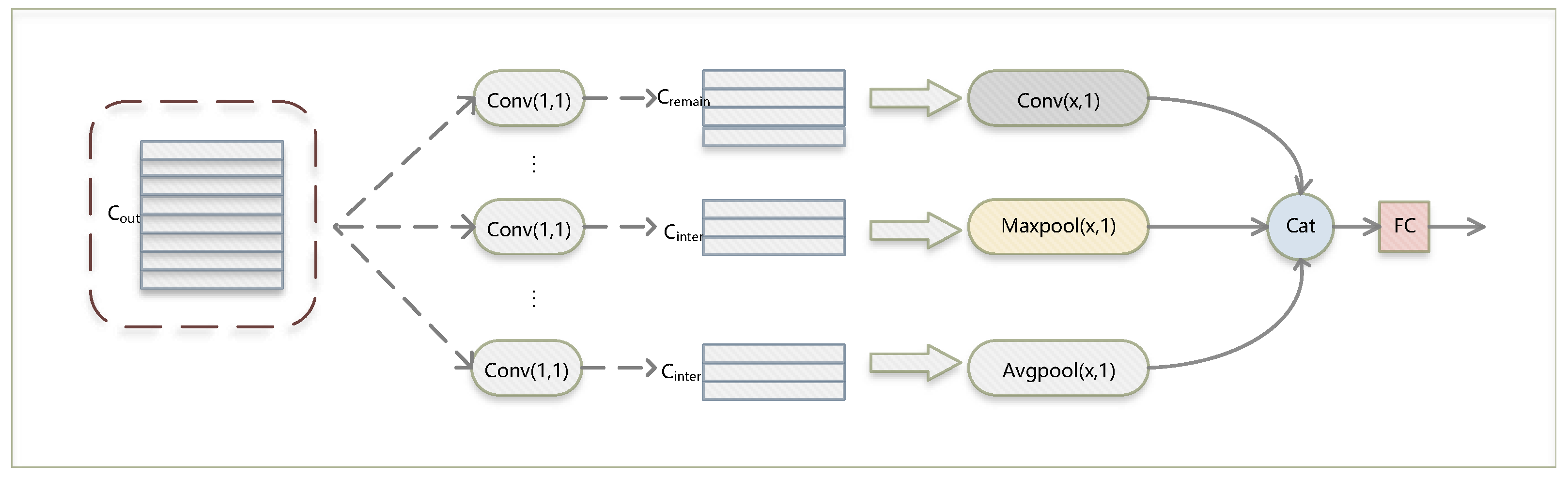
3.3. Multi-Scale Temporal Convolution Network

In terms of time, ST-GCN [36,37,38,39,40,41,42,43] introduced the innovative use of 2D convolution to extract temporal information, which has performed well in many fields. In the realm of gait recognition, skeleton-based models still employ this approach, but using a single-scale convolution for extracting temporal information is similar to capturing global features in the spatial dimension, which can cause the loss of temporal information. Drawing inspiration from global and local operations in the spatial domain, we propose a multi-scale temporal convolutional network (MTCN).

In the MTCN module, in order to inspect the final splicing of temporal features of different scales, we compute the intermediate and residual dimensions of the convolutional output of each scale based on the number of time windows of different sizes provided and the size of the output channels of the MTCN. The process of calculating the intermediate and remaining channels can be mathematically represented as follows:

$$C_{inter}=\lfloor \frac{C_{out}}{n}\rfloor$$

(4)

$$C_{rem\_inter}=C_{out}-C_{inter}\times n$$

(5)

where $C_{inter}$, $C_{rem\_inter}$, and $C_{out}$ represent the intermediate channel, remaining channel, and output channel of the MTCN, respectively. n is the amount of different scale windows.

After realizing the alignment of the intermediate channel, the remaining channel and the output channel, MTCN first downscales the gait features with different sizes of time scales and extracts the temporal information of the downscaled gait features by using kernels with different sizes (convolution kernel or pooling kernel), so as to obtain the temporal features with different scales. Finally, the temporal features of different scales are spliced along the channels to generate gait features with multi-scale temporal information, and then the weights of each channel are adjusted using the fully connected layer. The overall architecture of MTCN is shown in Figure 7. Its mathematical expression is as follows:

$$X_{out}=Concat(F\left(F_{1X1}\left(X_{in}\right)\right),G\left(F_{1X1}\left(X_{in}\right)\right),M\left(F_{1X1}\left(X_{in}\right)\right))$$

(6)

where $X_{in}$ and $X_{out}$ represent the input and output gait features, respectively. F(·) denotes the convolution operation on temporal features, G(·) represents the maximum pooling operation on temporal features, M(·) represents the average pooling operation on temporal features, and the output channel for the first time scale is $C_{re{m}_{i}nter}$, while the output channels for all other feature extraction operations are $C_{inter}$. Concat denotes channel concatenation.

The MTCN uses kernels of different sizes, including convolutional kernels and pooling kernels, to extract high-level gait features at different time scales. This enables the GaitMGL network to capture temporal features of different body part motion cycles within the gait cycle, thus allowing the GaitMGL network to extract more complete temporal information and thus enhance its overall performance.

4. Experiments

In this section, we assess the performance of our GaitMGL model on three popular datasets: CASIA-B [44], GREW [45], and Gait3D [46]. First, we introduce the basic information of the gait datasets and the training configurations corresponding to them. Subsequently, we compare GaitMGL with the SOTA gait network under the same experimental conditions. Finally, we perform ablation experiments on the proposed modules to visually examine the performance contribution of each module in GaitMGL.

4.1. Datasets

This paper utilized three mainstream gait datasets, including the widely used indoor dataset CASIA-B [44], as well as the extensively used GREW [45] and Gait3D [46], known for their diversity in wild environments.

Table 1. Statistical data on identity (#ID) and sequence (#Seq) for each dataset.

Dataset	Publication	Train Set		Test Set		Type
		#ID	#Seq	#ID	#Seq
CASIA-B	ICPR2006	74	8140	50	5500	NM, BG, CL
GREW	ICCV2021	20,000	102,887	6000	24,000	Diverse
Gait3D	CVPR2022	3000	18,940	1000	6369	Diverse

presents the statistical information related to the amount of identities and sequences contain in every dataset.

CASIA-B [44] is one of the most commonly used datasets in the field of gait recognition. It consists of 124 participants, and it recorded each individual’s walking gait in 10 different conditions (6 NM conditions—walking normally, 2 BG conditions—walking with a backpack, and 2 CL conditions—walking with thick clothing). Each gait condition was shot from 11 different viewpoints (from 0 to 180 degrees, with 18-degree intervals). To evaluate our network, we used the same protocol as [16]. The first 74 participants were trained as the training set and the remaining 50 participants were tested as the test set. The test set used the first four gaits in the normal walking condition as the gallery set and the rest of the gaits in the other conditions as the probe set. We extracted skeletal data from CASIA-B using a pre-trained HRNet [47] pose estimator.

GREW [45] is a wholesale wilderness dataset containing 26,345 objects with a total of 128,671 gait sequences. GREW has four different types of gait data with different attributes: silhouette, optical flow, 2D skeleton data, and 3D skeleton data. It is split into a train set, a validation set, a test set, and a disturbance set. The train set has 20,000 objects with 102,887 sequences. The validation set has 345 objects with 1784 sequences, and the test set includes 6000 objects with four sequences per identity. During the testing phase, each identity had two sequences as the probe and two other sequences as the gallery. The interference set contains 233,857 unidentified sequences. The interference set is an important feature that distinguishes GREW from other datasets and is a great challenge to the accuracy of gait recognition. In this study, we discard the interference set. The protocol in [45] is followed to evaluate the model and verify its performance in complex environments.

Gait3D [46] is a large outdoor dataset containing over 4000 subjects with more than 25,000 gait sequences shot by 39 cameras placed in a large supermarket. For the evaluation of GaitMGL, the dataset is split into a training set consisting of 3000 subjects, and the rest of subjects are designated as the test set. During the testing stage, one sequence is randomly selected as a probe from every subject in the test set, while all the other sequences from the same subjects form the gallery. This setup is commonly used in gait recognition experiments to assess the model’s performance in realistic scenarios.

Our implementation follows the official protocol, including training, testing, gallery, and probe set partitioning strategies. Rank-1 Accuracy is the dominant experimental evaluation metric.

4.2. Implementation Details

Table 2. Implementation configuration. The batch size N × S means N identities with S sequences per identity. The temporal scale (m,n) represents the size of the convolutional kernels at different temporal scales, and (‘Max’,3) represents a maximum pooling kernel with a pool size of (3,1).

Dataset	Temporal Scale	Batch Size	MultiStep Scheduler	Steps
CASIA-B	(9,1), (3,1), (‘MAX’,3)	10 × 6	(18,000)	20,000
GREW	(9,1), (3,1)	48 × 10	(30,000, 60,000, 90,000)	150,000
Gait3D	(9,1), (3,1)	48 × 10	(30,000)	32,000

presents the key hyper-parameters [48,49] used in our experiments on different datasets. During the training phase, we adopted the following settings:

• Training Batch Size. The training batch size is set as N × S, where N denotes the label number and S denotes the sequence number within every label. Specifically, the training batch size is set to 10 × 6 for the CASIA-B dataset and 48 × 10 for the GREW and Gait3D datasets.
• Optimizer. In the backpropagation process, we use the SGD optimizer and set 0.1 as the initial learning rate of the optimizer, 0.9 as the optimizer’s momentum, and set the weight decay to 0.0005. The scheduler settings are as follows. For the GREW dataset, the learning rate is to be reduced by a factor of 10 at steps of 30,000, 60,000, 90,000, and 120,000, for a total of 150,000 rounds of training. For the Gait3D and CASIA-B datasets, the decay is set at 30,000 and 18,000 batches, respectively, for a total of 32,000 and 20,000 rounds of training.
• Temporal scales. We tested different training timescales on the GREW and CASIA-B datasets (under normal walking conditions) to compare the accuracy of the models in order to determine the most suitable timescale for the datasets, and the experimental results are shown in

  Table 3. Accuracy (%) at different time scales in datasets GREW and CASIA-B (normal walking conditions).

  Dataset	Temporal Scale	Batch Size	Steps	Accuracy
  GREW	(9,1), (5,1), (3,1), (‘MAX’,3)	48 × 10	150,000	60.23
  	(9,1), (3,1), (‘MAX’,3)	48 × 10	150,000	62.71
  	(9,1), (3,1), (‘AVG’,3)	48 × 10	150,000	62.12
  	(9,1), (3,1)	48 × 10	150,000	63.12
  CASIA-B	(9,1), (3,1)	10 × 6	20,000	75.36
  	(9,1), (3,1), (‘MAX’,3)	10 × 6	20,000	63.12

  through experiments. We select the (3,1) and (9,1) convolution kernels as time scales for the GREW and Gait3D datasets. For the CASIA-B dataset, the (3,1) and (9,1) convolution kernels as well as the maximum pooling kernel of (3,1) are selected as time scales.
• Data augmentation. Considering real data and errors from pose estimation, we added joint noise with a variance of 0.25 to the coordinates of each joint.
• Other configurations. We set the loss function threshold to 0.1. The network fully connected mapping layer has an input dimension of 256 and an output dimension of 128.

All experimental procedures were executed on a single NVIDIA GeForce GTX 2070 GPU (TSMC, Taiwan, China) using the PyTorch 1.12.1 + cu113 framework.

4.3. Comparison with State-Of-The-Art Methods

To demonstrate the performance of our proposed model, we will contrast it with the SOTA method on three commonly used datasets: CASIA-B, GREW, and Gait3D.

Evaluation on CASIA-B. First, we compared the results of model-based methods on CASIA-B, as shown in

Table 4. Accuracy (%) from 0 to 180 rank-1 under three different walking conditions on the CASIA-B dataset compared to existing model-based networks. ‘NM’, ‘BG’, and ‘CL’ denote the three different walking conditions of normal walking, backpack walking, and walking with a jacket, respectively.

Gallery		0°–180°											Mean
Probe		0°	18°	36°	54°	72°	90°	108°	126°	144°	162°	180°
NM	PoseGait	55.3	69.6	73.9	75	68	68.2	71.1	72.9	76.1	70.4	55.4	68.7
	GaitGraph	85.3	88.5	91	92.5	87.2	86.5	88.4	89.2	87.9	85.9	81.9	87.7
	GaitGraph2	78.5	82.9	85.8	85.6	83.1	81.5	84.3	83.2	84.2	81.6	71.8	82
	Ours	79.9	87	85.6	85.4	86.9	87.6	87.1	88	85.8	86.4	84.2	85.8
BG	PoseGait	35.3	47.2	52.4	46.9	45.5	43.9	46.1	48.1	49.4	43.6	31.1	44.5
	GaitGraph	75.8	76.7	75.9	76.1	71.4	73.9	78	74.7	75.4	75.4	69.2	74.8
	GaitGraph2	69.9	75.9	78.1	79.3	71.4	71.7	74.3	76.2	73.2	73.4	61.7	73.2
	Ours	70.9	75.6	77.9	78.9	77.4	76	76.6	76.1	77.9	79.6	67.4	75.9
CL	PoseGait	24.3	29.7	41.3	38.8	38.2	38.5	41.6	44.9	42.2	33.4	22.5	36
	GaitGraph	69.6	66.1	68.8	67.2	64.5	62	69.5	65.6	65.7	66.1	64.3	66.3
	GaitGraph2	57.1	61.1	68.9	66	67.8	65.4	68.1	67.2	63.7	63.6	50.4	63.6
	Ours	68.5	71.4	73.1	70.5	71.8	68.2	71.9	69.5	70.4	73.4	68	70.6

. Observing the experimental results, it can be noticed that, compared to the frontal view angles (0° and 180°) and the lateral view angle (90°), all model-based gait recognition methods exhibit better performance in terms of the tilt angle. We speculate that under the frontal and lateral view angles, the information conveyed by the skeletal data is limited, which restricts their performance. Furthermore, our model, GaitMGL, ranks second only to gaitgraph under normal walking conditions and outperforms all previous model-based gait recognition methods in other walking conditions. This demonstrates that our GaitMGL model exhibits stronger robustness under varying gait-walking conditions. Meanwhile, we are concerned that the accuracy of our GaitGML is lower than that of Gaitgraph under normal walking conditions, which we conjecture is due to the fact that joint flow has a greater impact on the accuracy during normal walking; however, our multiple branching attenuates the feature expression of joint flow. Therefore, we can pay more attention to the fusion of multi-branching in the subsequent research, so that it can adaptively learn the weight of the influence of each stream on the final result. Subsequently, we compared our results with appearance-based methods on the CASIA-B dataset. The experimental results can be found in

Table 5. Mean accuracy (%) of Rank-1, Rank-5, Rank-10, and Rank-20 in the GREW dataset compared to other model-based methods.

Methods	Publication	Type			Mean
		NM#	BG#	CL#
GaitSet [14]	AAAI 2019	95.8	90	75.4	87
GaitPart [15]	CVPR 2020	96.1	90.7	78.7	88.5
GaitGL [16]	ICCV 2021	97.4	94.5	83.8	91.9
GaitBase [19]	CVPR 2023	97.6	94	77.4	89.6
GaitMGL	Ours	85.8	75.9	70.6	77.4

. The results indicate that appearance-based recognition methods continue to lead in accuracy on the indoor CASIA-B dataset. Two reasons for this are as follows. 1. Skeletal data at certain specific angles (0°, 90°, and 180°) limit the accuracy of model-based recognition methods. 2. Pose estimation networks are less accurate for individuals wearing coats and carrying bags. Additionally, the experimental results also demonstrate that our model has helped bridge the gap between model-based methods and appearance-based recognition methods.

Evaluation on GREW. We simultaneously compared the current state-of-the-art model-based and appearance-based recognition methods on the large-scale GREW dataset. The experimental results can be found in

Table 6. GREW in terms of averaged Rank-1, Rank-5, Rank-10, and Rank-20 accuracies (%) compared to other model-based approaches.

Methods	Publication	Rank-1	Rank-5	Rank-10	Rank-20
PoseGait [22]	PR 2020	0.23	1.05	2.23	4.28
GaitGraph1 [23]	ICIP 2021	1.31	3.46	5.08	7.51
GaitGraph2 [24]	CVPR 2022	33.54	49.45	56.28	61.92
GaitMGL	Ours	63.12	79.75	84.87	88.60

and

Table 7. Mean accuracy (%) for Rank-1, Rank-5, Rank-10, and Rank-20 for GREW compared to other appearance-based methods.

Methods	Publication	Rank-1	Rank-5	Rank-10	Rank-20
GaitSet [14]	AAAI 2019	46.28	63.58	70.26	76.82
GaitPart [15]	CVPR 2020	44.01	60.68	67.25	73.47
GaitGL [16]	ICCV 2022	47.28	63.56	69.32	74.18
GaitBase [19]	CVPR 2023	60.10	75.40	80.38	84.16
GaitMGL	Ours	63.12	79.75	84.87	88.60

. We can observe that our method outperforms all current gait recognition methods on the GREW dataset. When compared to model-based gait recognition methods, our approach achieves nearly double the accuracy improvement compared to the recent GaitGraph2. This shows that our model is robust in complex outdoor environments, and also verifies that gait features with global–local spatial information and multi-scale temporal information are more advantageous in representing gait characteristics. Furthermore, in comparison to appearance-based recognition methods, our model’s accuracy surpasses that of the current best appearance-based gait recognition methods. These pleasantly surprising results indicate that model-based gait recognition methods still hold significant research value in the field of gait recognition.

Evaluation on Gait3D. We compared model-based gait recognition methods on the recently released Gait3D dataset, and the experimental results are shown in

Table 8. Averaged Rank-1, Rank-5, mAP, and mINP accuracies in percent on Gait3D compared with other model-based methods.

Methods	Publication	Rank-1	Rank-5	mAP	mINP
PoseGait [22]	PR 2020	0.24	1.08	0.47	0.34
GaitGraph1 [23]	ICIP 2021	6.25	16.23	5.18	2.42
GaitGraph2 [24]	CVPR 2022	11.20	24.00	-	-
GaitMGL	Ours	22.70	42.70	18.65	9.48

. We observed that despite surpassing the performance of GaitGraph2, our model still achieved a relatively low accuracy on Gait3D. During the experiments, we also noticed that our model tends to overfit on Gait3D. The reason for this could be attributed to the limited diversity of samples in the smaller dataset, which does not support the learning of more extensive gait variation features. Specifically, the skeletal information in the smaller dataset is limited, making it easier for our model to fit together during the learning process, which in turn affects its performance.

4.4. Ablation Studies

In this section, in order to verify the effectiveness of our proposed blocks GLGCN and MTCN, we perform ablation experiments. We used GaitGraph2 as our baseline network and made adjustments to its loss function, data augmentation, and TTA (Test-Time Augmentation) scheduling strategy. The adjusted baseline network achieved an accuracy of 57.74% on GREW. Furthermore, all hyperparameters in the ablation experiments were kept consistent with the parameters listed in Table 2 for GREW.

Evaluation of the GLGCN module. We were inspired by GaitGL and started focusing on local features that were previously overlooked by model-based recognition methods. As a result, we introduced the Global–Local Extractor, GLGCN. GLGCN divides the original sequence into upper and lower body parts, extracting local information separately, and then fuses it with global features to generate the global–local features. We conducted ablation experiments on this aspect, and the experimental data are presented in

Table 9. Recognition accuracy of different blocks on GREW dataset (%).

Methods	Rank-1	Rank-5	Rank-10	Rank-20
baseline	57.74	75.87	81.43	85.93
baseline + GLGCN	62.10	79.00	84.20	88.30
baseline + MTCN	60.65	78.33	83.64	87.72
ours (MTCN + GLGCN)	63.12	79.75	84.87	88.60

. The accuracy of the baseline + GLGCN reached 62.10%, which is a 4.36% improvement over the baseline network. This result indicates that GLGCN’s extraction of local features is helpful in improving accuracy for model-based recognition methods.

Evaluation of the MTCN module. In order to solve the issue of losing temporal sequence information caused by single-scale time extraction, we draw inspiration from global and local operations in the spatial domain and propose the MTCN module. This module provides solution ideas in coping with the problem of local motion cycle inconsistency and enhances the flexibility of the model-based recognition network in processing temporal sequences. As shown in Table 9, the accuracy of the baseline+ MTCN reaches 60.65%, which is about 2.82% better than the baseline network. The experimental data show that MTCN is beneficial for enhancing the accuracy of the network.

Evaluation of the MTCN and GLGCN modules. We simultaneously integrated the GLGCN module and the MTCN module, and the experimental results are shown in Table 9. Our model, by extracting global–local information and multi-scale temporal information, achieved a score of 63.12% on the GREW dataset, surpassing the current best model-based networks. Furthermore, the experiments confirm the validity of our proposed GLGCN and MTCN blocks.

5. Conclusions

In this study, we present a new gait recognition network named GaitMGL, designed to extract more comprehensive gait features. GaitMGL is constructed based on multiple MGL (Multi-scale Temporal and Global–Local Spatial Extraction Module) modules, specifically consisting of a global–local spatial feature extractor named GLGCN for extracting both global and local information, along with a multi-scale temporal feature extractor known as MTCN for capturing temporal information at multiple scales. The GLGCN divides the skeleton into upper and lower limbs, extracting their information to generate local gait features, which are then fused with the global skeleton feature to obtain a high-level representation of global–local gait features. Meanwhile, the MTCN utilizes time windows of different sizes to extract more complete temporal information. Our model has been thoroughly evaluated on three prominent datasets, with the experimental results indicating that our model GaitMGL outperforms all current model-based gait recognition methods in three publicly available datasets (CASIA-B, GREW, Gait3D), especially in the outdoor dataset GREW, where our accuracy improves by nearly two times compared to existing methods. Furthermore, the results of ablation experiments validate the effectiveness of our proposed GLGCN and MTCN modules. In the process of experimentation, we found that for GaitMGL, under a certain specific condition, the performance of multiple branches in GaitMGL is not as good as that of a single jointed stream, and we speculate that it is because the process of multibranch fusion did not take into account the influence of each stream on the results. Based on this, our subsequent research will be centered on multi-branch fusion.

References

1. Ding, W.; Abdel-Basset, M.; Hawash, H.; Moustafa, N. Interval type-2 fuzzy temporal convolutional autoencoder for gait-based human identification and authentication. Inf. Sci. 2022, 597, 144–165. [Google Scholar] [CrossRef]
2. Yogarajah, P.; Chaurasia, P.; Condell, J.; Prasad, G. Enhancing gait based person identification using joint sparsity model and 1-norm minimization. Inf. Sci. 2015, 308, 3–22. [Google Scholar] [CrossRef]
3. Bronstein, A.M.; Bronstein, M.M.; Kimmel, R. Three-dimensional face recognition. Int. J. Comput. Vis. 2005, 64, 5–30. [Google Scholar] [CrossRef]
4. Yang, J.; Xiong, N.; Vasilakos, A.V.; Fang, Z.; Park, D.; Xu, X.; Yoon, S.; Xie, S.; Yang, Y. A fingerprint recognition scheme based on assembling invariant moments for cloud computing communications. IEEE Syst. J. 2011, 5, 574–583. [Google Scholar] [CrossRef]
5. Shu, L.; Zhang, Y.; Yu, Z.; Yang, L.T.; Hauswirth, M.; Xiong, N. Context-aware cross-layer optimized video streaming in wireless multimedia sensor networks. J. Supercomput. 2010, 54, 94–121. [Google Scholar] [CrossRef]
6. Hu, W.J.; Fan, J.; Du, Y.X.; Li, B.S.; Xiong, N.; Bekkering, E. MDFC–ResNet: An agricultural IoT system to accurately recognize crop diseases. IEEE Access 2020, 8, 115287–115298. [Google Scholar] [CrossRef]
7. Zhao, J.; Huang, J.; Xiong, N. An effective exponential-based trust and reputation evaluation system in wireless sensor networks. IEEE Access 2019, 7, 33859–33869. [Google Scholar] [CrossRef]
8. Zeng, Y.; Sreenan, C.J.; Xiong, N.; Yang, L.T.; Park, J.H. Connectivity and coverage maintenance in wireless sensor networks. J. Supercomput. 2010, 52, 23–46. [Google Scholar] [CrossRef]
9. Müller, R.; Kornblith, S.; Hinton, G.E. When does label smoothing help? Adv. Neural Inf. Process. Syst. 2019, 32. [Google Scholar]
10. Fang, W.; Li, Y.; Zhang, H.; Xiong, N.; Lai, J.; Vasilakos, A.V. On the throughput-energy tradeoff for data transmission between cloud and mobile devices. Inf. Sci. 2014, 283, 79–93. [Google Scholar] [CrossRef]
11. Luo, H.; Gu, Y.; Liao, X.; Lai, S.; Jiang, W. Bag of tricks and a strong baseline for deep person re-identification. In Proceedings of the IEEE/CVF Conference on Computer Vision and Pattern Recognition Workshops, Long Beach, CA, USA, 16–17 June 2019. [Google Scholar]
12. Bieliński, A.; Rojek, I.; Mikołajewski, D. Comparison of Selected Machine Learning Algorithms in the Analysis of Mental Health Indicators. Electronics 2023, 12, 4407. [Google Scholar] [CrossRef]
13. Yao, B.; He, H.; Kang, S.; Chao, Y.; He, L. A Review for the Euler Number Computing Problem. Electronics 2023, 12, 4406. [Google Scholar] [CrossRef]
14. Chao, H.; He, Y.; Zhang, J.; Feng, J. Gaitset: Regarding gait as a set for cross-view gait recognition. In Proceedings of the AAAI Conference on Artificial Intelligence, Honolulu, HI, USA, 27 January–1 February 2019; Volume 33, pp. 8126–8133. [Google Scholar]
15. Fan, C.; Peng, Y.; Cao, C.; Liu, X.; Hou, S.; Chi, J.; Huang, Y.; Li, Q.; He, Z. Gaitpart: Temporal part-based model for gait recognition. In Proceedings of the IEEE/CVF Conference on Computer Vision and Pattern Recognition, Seattle, WA, USA, 13–19 June 2020; pp. 14225–14233. [Google Scholar]
16. Lin, B.; Zhang, S.; Wang, M.; Li, L.; Yu, X. Gaitgl: Learning discriminative global-local feature representations for gait recognition. arXiv 2022, arXiv:2208.01380. [Google Scholar]
17. Huang, Z.; Xue, D.; Shen, X.; Tian, X.; Li, H.; Huang, J.; Hua, X.S. 3D local convolutional neural networks for gait recognition. In Proceedings of the IEEE/CVF International Conference on Computer Vision, Nashville, TN, USA, 20–25 June 2021; pp. 14920–14929. [Google Scholar]
18. Liang, J.; Fan, C.; Hou, S.; Shen, C.; Huang, Y.; Yu, S. Gaitedge: Beyond plain end-to-end gait recognition for better practicality. In Proceedings of the European Conference on Computer Vision, Tel Aviv, Israel, 23–27 October 2022; Springer: Berlin/Heidelberg, Germany, 2022; pp. 375–390. [Google Scholar]
19. Fan, C.; Liang, J.; Shen, C.; Hou, S.; Huang, Y.; Yu, S. OpenGait: Revisiting Gait Recognition Towards Better Practicality. In Proceedings of the IEEE/CVF Conference on Computer Vision and Pattern Recognition, Vancouver, BC, Canada, 18–22 June 2023; pp. 9707–9716. [Google Scholar]
20. Dou, H.; Zhang, P.; Su, W.; Yu, Y.; Li, X. Metagait: Learning to learn an omni sample adaptive representation for gait recognition. In Proceedings of the European Conference on Computer Vision, Glasgow, UK, 23 August 2022; Springer: Berlin/Heidelberg, Germany, 2022; pp. 357–374. [Google Scholar]
21. Wang, M.; Guo, X.; Lin, B.; Yang, T.; Zhu, Z.; Li, L.; Zhang, S.; Yu, X. DyGait: Exploiting Dynamic Representations for High-performance Gait Recognition. arXiv 2023, arXiv:2303.14953. [Google Scholar]
22. Liao, R.; Yu, S.; An, W.; Huang, Y. A model-based gait recognition method with body pose and human prior knowledge. Pattern Recognit. 2020, 98, 107069. [Google Scholar] [CrossRef]
23. Teepe, T.; Khan, A.; Gilg, J.; Herzog, F.; Hörmann, S.; Rigoll, G. Gaitgraph: Graph convolutional network for skeleton-based gait recognition. In Proceedings of the 2021 IEEE International Conference on Image Processing (ICIP), Anchorage, AK, USA, 19–22 September 2021; pp. 2314–2318. [Google Scholar]
24. Teepe, T.; Gilg, J.; Herzog, F.; Hörmann, S.; Rigoll, G. Towards a deeper understanding of skeleton-based gait recognition. In Proceedings of the IEEE/CVF Conference on Computer Vision and Pattern Recognition, New Orleans, LA, USA, 18–24 June 2022; pp. 1569–1577. [Google Scholar]
25. Lin, B.; Liu, Y.; Zhang, S. Gaitmask: Mask-based model for gait recognition. In Proceedings of the BMVC, Virtual, 22–25 November 2021; pp. 1–12. [Google Scholar]
26. Xu, C.; Makihara, Y.; Li, X.; Yagi, Y. Occlusion-aware human mesh model-based gait recognition. IEEE Trans. Inf. Forensics Secur. 2023, 18, 1309–1321. [Google Scholar] [CrossRef]
27. Liao, R.; Cao, C.; Garcia, E.B.; Yu, S.; Huang, Y. Pose-based temporal-spatial network (PTSN) for gait recognition with carrying and clothing variations. In Proceedings of the Biometric Recognition: 12th Chinese Conference, CCBR 2017, Shenzhen, China, 28–29 October 2017; Proceedings 12. Springer: Berlin/Heidelberg, Germany, 2017; pp. 474–483. [Google Scholar]
28. Wang, L.; Chen, J.; Chen, Z.; Liu, Y.; Yang, H. Multi-stream part-fused graph convolutional networks for skeleton-based gait recognition. Connect. Sci. 2022, 34, 652–669. [Google Scholar] [CrossRef]
29. Sokolova, A.; Konushin, A. Pose-based deep gait recognition. IET Biom. 2019, 8, 134–143. [Google Scholar] [CrossRef]
30. Pan, H.; Chen, Y.; Xu, T.; He, Y.; He, Z. Toward Complete-View and High-Level Pose-Based Gait Recognition. IEEE Trans. Inf. Forensics Secur. 2023, 18, 2104–2118. [Google Scholar] [CrossRef]
31. Santos, C.F.G.d.; Oliveira, D.D.S.; Passos, L.A.; Pires, R.G.; Santos, D.F.S.; Valem, L.P.; Moreira, T.P.; Santana, M.C.S.; Roder, M.; Papa, J.P.; et al. Gait recognition based on deep learning: A survey. arXiv 2022, arXiv:2201.03323. [Google Scholar]
32. Shiraga, K.; Makihara, Y.; Muramatsu, D.; Echigo, T.; Yagi, Y. Geinet: View-invariant gait recognition using a convolutional neural network. In Proceedings of the 2016 International Conference on Biometrics (ICB), Halmstad, Sweden, 13–16 June 2016; pp. 1–8. [Google Scholar]
33. Fang, H.S.; Xie, S.; Tai, Y.W.; Lu, C. Rmpe: Regional multi-person pose estimation. In Proceedings of the IEEE International Conference on Computer Vision, Venice, Italy, 22–29 October 2017; pp. 2334–2343. [Google Scholar]
34. Cao, Z.; Simon, T.; Wei, S.E.; Sheikh, Y. Realtime multi-person 2d pose estimation using part affinity fields. In Proceedings of the IEEE Conference on Computer Vision and Pattern Recognition, Honolulu, HI, USA, 21–26 July 2017; pp. 7291–7299. [Google Scholar]
35. Liu, Z.; Zhang, H.; Chen, Z.; Wang, Z.; Ouyang, W. Disentangling and unifying graph convolutions for skeleton-based action recognition. In Proceedings of the IEEE/CVF Conference on Computer Vision and Pattern Recognition, Seattle, WA, USA, 13–19 June 2020; pp. 143–152. [Google Scholar]
36. Yan, S.; Xiong, Y.; Lin, D. Spatial temporal graph convolutional networks for skeleton-based action recognition. In Proceedings of the AAAI Conference on Artificial Intelligence, New Orleans, LA, USA, 2–7 February 2018; Volume 32. [Google Scholar]
37. Duan, H.; Wang, J.; Chen, K.; Lin, D. Pyskl: Towards good practices for skeleton action recognition. In Proceedings of the 30th ACM International Conference on Multimedia, Lisbon, Portugal, 10 October 2022; pp. 7351–7354. [Google Scholar]
38. Li, G.; Muller, M.; Thabet, A.; Ghanem, B. Deepgcns: Can gcns go as deep as cnns? In Proceedings of the IEEE/CVF International Conference on Computer Vision, Seoul, Republic of Korea, 27 October–2 November 2019; pp. 9267–9276. [Google Scholar]
39. Song, Y.; Li, W.; Dai, G.; Shang, X. Advancements in Complex Knowledge Graph Question Answering: A Survey. Electronics 2023, 12, 4395. [Google Scholar] [CrossRef]
40. Cheng, K.; Zhang, Y.; He, X.; Chen, W.; Cheng, J.; Lu, H. Skeleton-based action recognition with shift graph convolutional network. In Proceedings of the IEEE/CVF Conference on Computer Vision and Pattern Recognition, Seattle, WA, USA, 13–19 June 2020; pp. 183–192. [Google Scholar]
41. Duan, H.; Wang, J.; Chen, K.; Lin, D. DG-STGCN: Dynamic spatial-temporal modeling for skeleton-based action recognition. arXiv 2022, arXiv:2210.05895. [Google Scholar]
42. Chen, Y.; Zhang, Z.; Yuan, C.; Li, B.; Deng, Y.; Hu, W. Channel-wise topology refinement graph convolution for skeleton-based action recognition. In Proceedings of the IEEE/CVF International Conference on Computer Vision, Montreal, BC, Canada, 11–17 October 2021; pp. 13359–13368. [Google Scholar]
43. Hou, J.; Wang, G.; Chen, X.; Xue, J.H.; Zhu, R.; Yang, H. Spatial-temporal attention res-TCN for skeleton-based dynamic hand gesture recognition. In Proceedings of the European Conference on Computer Vision (ECCV) Workshops, Munich, Germany, 8–14 September 2018. [Google Scholar]
44. Yu, S.; Tan, D.; Tan, T. A framework for evaluating the effect of view angle, clothing and carrying condition on gait recognition. In Proceedings of the 18th International Conference on Pattern Recognition (ICPR’06), Hong Kong, China, 20–24 August 2006; Volume 4, pp. 441–444. [Google Scholar]
45. Zhu, Z.; Guo, X.; Yang, T.; Huang, J.; Deng, J.; Huang, G.; Du, D.; Lu, J.; Zhou, J. Gait recognition in the wild: A benchmark. In Proceedings of the IEEE/CVF International Conference on Computer Vision, Montreal, BC, Canada, 11–17 October 2021; pp. 14789–14799. [Google Scholar]
46. Zheng, J.; Liu, X.; Liu, W.; He, L.; Yan, C.; Mei, T. Gait recognition in the wild with dense 3d representations and a benchmark. In Proceedings of the IEEE/CVF Conference on Computer Vision and Pattern Recognition, New Orleans, LA, USA, 18–24 June 2022; pp. 20228–20237. [Google Scholar]
47. Sun, K.; Xiao, B.; Liu, D.; Wang, J. Deep high-resolution representation learning for human pose estimation. In Proceedings of the IEEE/CVF Conference on Computer Vision and Pattern Recognition, Long Beach, CA, USA, 15–20 June 2019; pp. 5693–5703. [Google Scholar]
48. Wang, Y.; Fang, W.; Ding, Y.; Xiong, N. Computation offloading optimization for UAV-assisted mobile edge computing: A deep deterministic policy gradient approach. Wirel. Netw. 2021, 27, 2991–3006. [Google Scholar] [CrossRef]
49. Kang, L.; Chen, R.S.; Xiong, N.; Chen, Y.C.; Hu, Y.X.; Chen, C.M. Selecting hyper-parameters of Gaussian process regression based on non-inertial particle swarm optimization in Internet of Things. IEEE Access 2019, 7, 59504–59513. [Google Scholar] [CrossRef]
Figure 1. The distinct expressions of the upper and lower limbs in human gait during walking. The line graph inside the orange dashed line corresponds to the periodogram of the arm movement, and the line graph inside the blue dashed line corresponds to the periodogram of the leg movement.
Electronics 13 00257 g001
Figure 2. The different cyclical patterns of upper and lower limbs during human gait.
Electronics 13 00257 g002
Figure 3. The overall process of GaitMGL.
Electronics 13 00257 g003
Figure 4. The overall process of multi-branch extraction.The red dashed portion is the feature after channel splicing.
Electronics 13 00257 g004
Figure 5. The structure diagram of the MGL. In GLGCN, GGCN and LGCN represent the global extractor and local extractor, respectively. The different colored blocks in MTCN represent the processing of different time scales.
Electronics 13 00257 g005
Figure 6. The overall process of GLGCN. C, T, and V represent the channel, time dimension, and joint point dimension, respectively. V u p and V l o w are the upper and lower limb joint points obtained by slicing the features along V. A, A u p , and A l o w , respectively, represent the prior matrices, the prior matrix for the upper limb joints, and the prior matrix for the lower limb joints, respectively. BN denotes batch normalization.
Electronics 13 00257 g006
Figure 7. The overall process of MTCN. C o u t , C i n t e r , and C r e m i a n represent the output channel, intermediate channel and remaining channel of MTCN, respectively. Conv(1, 1) denotes a 1 × 1 convolution, Maxpool(x, 1) denotes maximum pooling with a pooling kernel of (x, 1), Avgpool(x, 1) denotes the average pooling with a pooling kernel of (x, 1), FC denotes fully connected layer.
Electronics 13 00257 g007