TCα-PIA: A Personalized Social Network Anonymity Scheme via Tree Clustering and α-Partial Isomorphism

Abstract

Social networks have become integral to daily life, allowing users to connect and share information. The efficient analysis of social networks benefits fields such as epidemiology, information dissemination, marketing, and sentiment analysis. However, the direct publishing of social networks is vulnerable to privacy attacks such as typical 1-neighborhood attacks. This attack can infer the sensitive information of private users using users’ relationships and identities. To defend against these attacks, the k-anonymity scheme is a widely used method for protecting user privacy by ensuring that each user is indistinguishable from at least $k-1$ other users. However, this approach requires extensive modifications that compromise the utility of the anonymized graph. In addition, it applies uniform privacy protection, ignoring users’ different privacy preferences. To address the above challenges, this paper proposes an anonymity scheme called TC$\alpha$-PIA (Tree Clustering and $\alpha$-Partial Isomorphism Anonymization). Specifically, TC$\alpha$-PIA first constructs a similarity tree to capture subgraph feature information at different levels using a novel clustering method. Then, it extracts the different privacy requirements of each user based on the node cluster. Using the privacy requirements, it employs an $\alpha$-partial isomorphism-based graph structure anonymization method to achieve personalized privacy requirements for each user. Extensive experiments on four public datasets show that TC$\alpha$-PIA outperforms other alternatives in balancing graph privacy and utility.

1. Introduction

With the rise of social platforms like WeChat and Twitter, a vast number of users have joined, forming large-scale social networks and generating massive amounts of data. This published data has significant value, and social network operators often share user relationship graphs and other information with third parties [1] to facilitate data analysis and mining, social group analysis, and personalized recommendations. However, directly publishing unprocessed data poses significant privacy risks for things such as privacy theft attacks, identity attacks, and social relationship inference attacks.

To protect user privacy in social networks, various privacy-preserving mechanisms have been widely employed, such as naïve anonymization mechanisms [2], k-anonymity [3,4,5], encryption techniques [6,7,8], and differential privacy [9,10,11,12]. Naïve anonymization replaces identity information in social network data with random pseudo-identities, effectively defending against zero-knowledge adversaries. However, it fails to protect against attackers who possess knowledge of the graph structure. Encryption techniques encrypt social network data to protect the privacy of sensitive information. However, these techniques are costly in terms of data encryption, decryption, and key management. Additionally, they lack flexibility and are vulnerable to privacy attacks once the key has been compromised. Differential privacy introduces noise into data and has been widely applied in data mining, machine learning, and data analysis due to its theoretical security and ease of implementation [13]. However, the added noise can reduce the accuracy of data analysis, affecting the practical utility of the data. In contrast, k-anonymity is based on the concept of data generalization, ensuring that each node in the graph is indistinguishable from at least $k-1$ other nodes by adding or deleting nodes and/or edges in the social network graph. This significantly reduces the possibility of attackers identifying users to 1/k. In summary, k-anonymity provides stronger anonymity than naïve mechanisms, avoids the high computational overhead and complex key management required by encryption techniques, and is easier to understand and implement compared to differential privacy.

Many efforts have been made to develop an efficient k-anonymity scheme. For example, Yazdanjue et al. [14] proposed an EDPSO algorithm based on k-anonymity. This algorithm clusters nodes and edges in the network into super-nodes and super-edges to protect the structural information of individuals, thereby protecting user privacy. Although this approach effectively protects structural privacy, it does not address the personalized anonymization needs of users, indicating potential for further improvement. Wang et al. [15] proposed the GCA-DA algorithm. This algorithm clusters nodes by quantifying the distance and attribute similarity between them, ensuring that each cluster contains at least k nodes before anonymizing them. It protects privacy through attribute generalization and distinguishes between numerical and non-numerical attributes to maintain data usability. While this approach enhances clustering quality, it lacks flexibility. Zhang et al. [16] introduced a social network privacy protection scheme called GPPS. This scheme first employs degree-based graph entropy and spectral clustering algorithms for cluster nodes, and then adjusts 1-neighborhood graphs using a maximum weight bipartite matching method to achieve k-anonymity. However, it does not focus on graph isomorphism and fails to consider different user privacy requirements, indicating that the scheme can be further improved.

Therefore, to effectively address the aforementioned problems and balance the privacy and utility of the anonymity scheme in social networks, this paper proposes a similarity tree clustering method and an $\alpha$-partial isomorphism anonymization scheme based on the concepts of clustering and isomorphism. First, we perform node clustering using a similarity tree. We calculate the structural similarity between nodes and construct the similarity tree based on the obtained results. Next, we perform a unification operation on each cluster after the initial clustering to prevent attackers from exploiting differences in the number of users across clusters for identification attacks. Finally, we propose an $\alpha$-partial isomorphism anonymization algorithm based on the concept of isomorphism. This method addresses different structural privacy requirements of users by using mapping relationships and mapping matrices. It aims to minimize modifications to the graph and improve the utility of the anonymized graph. Specifically, the main contributions of this paper are as follows.

• We propose a new combined criterion for node similarity calculation to capture structural features of the 1-neighborhood subgraph from different factors, providing a foundation for subsequent node clustering.
• We propose a similarity tree clustering method that constructs a connection relationship tree based on similarity results. This method better reveals correlations between users, achieves node clustering, and effectively mitigates information difference attacks.
• We propose an $\alpha$-partial isomorphism ($0<\alpha \le 1$) anonymization algorithm based on the concept of isomorphism, which meets users’ personalized structural privacy requirements while enhancing the utility of anonymized graphs.
• Based on the real datasets, the experimental comparison between the proposed TC$\alpha$-PIA scheme and the same type of scheme is implemented. The results show that TC$\alpha$-PIA has higher utility. In particular, the excellent performance in information loss fully indicates that TC$\alpha$-PIA has less impact on the original graph and better preserves the utility of the anonymized graph.

The rest of the paper is organized as follows. Section 2 reviews the representative-related works. Section 3 introduces the privacy protection scenarios and problem definitions for social networks. Section 4 details the newly proposed TC$\alpha$-PIA. Section 5 evaluates the protocols and completes the experimental comparisons. Section 6 summarizes the work of this paper and gives future work.

2. Related Works

Commonly used privacy-preserving methods in social network graph publishing include k-anonymity, the perturbation of nodes and edges, and differential privacy.

Degree protection. k-anonymity ensures that each record or individual in the dataset is indistinguishable from at least $k-1$ other records or individuals. However, besides protecting users’ identity, it is equally important to protect the privacy of users’ degrees in social networks. This prevents attackers from using degrees for re-identification attacks. Therefore, it is necessary to ensure the privacy of each node’s degree in social networks. Therefore, k-degree anonymity is further proposed on the basis of k-anonymity. Specifically, there exist at least $k-1$ nodes with the same degree to ensure the indistinguishability of node degrees, effectively defending against node degree attacks [17,18]. Based on this concept, Lu et al. [19] further proposed a fast k-anonymization method, named FKDA. This method anonymizes the degree sequence of a graph by adding extra edges. Hartung et al. [20] further improved this approach by proposing an improved heuristic algorithm. This algorithm works in two stages, including anonymizing degree sequences and achieving k-anonymous degree sequences. It minimizes the number of edges added to a social network graph to achieve k-anonymity. However, these methods cannot preserve anonymized graph utility. To balance graph anonymity and utility, Casas-Roma et al. [21] proposed the UMGA k-degree anonymization algorithm. The method first creates a k-degree anonymous degree sequence, and then modifies edges with low centrality to maintain network integrity, reduce information loss, and enhance graph utility. Sharma et al. [22] extended the k-anonymization based on clustering. The method first clusters nodes according to the connection relationship between nodes and then places nodes with the same degree in the same group, reducing the modifications to the nodes. It performs better in terms of utility preservation. Kiabod et al. [23] proposed a one-time scan algorithm and reduced the anonymization overhead by creating a tree structure. This approach allows nodes to be grouped based on degree without having to perform anonymization from scratch. In addition, the method improves the utility of anonymized graphs by using participation and minimal path criteria for adding and deleting edges. Building on their previous work [23], Kiabod et al. [24] proposed the NaFa4KDA algorithm to further improve the speed of graph modification. This algorithm creates an anonymized degree sequence by clustering nodes and assigning target degrees, and enhances graph anonymity by computing and selecting edges with minimal impact for deletion during the modification process. In the pursuit of user privacy and improved data utility, Xiang et al. [25] designed a new degree-anonymized sequence generation algorithm using depth-first search, which reduces the differences between the anonymized graph and the original graph. Overall, k-degree anonymity effectively extends k-anonymity by strategically utilizing graph features, including node degrees and edges, through node groupings and edge modifications, thus achieving a balance between privacy protection and data utility in social network graphs.

Neighbor protection. Researchers have incorporated more information about the graph structure into the anonymization processes. A typical method is k-neighborhood anonymity [26,27], which processes the node neighbors and ensures that each node has at least k similar neighbors. Zhou et al. [28] proposed 1-neighborhood anonymity for the social network graph, meaning that the graph is anonymized so that each node in the graph has at least the same $k-1$ 1-hop neighbors. However, this scheme requires the continuous addition of fake edges to the nodes of the graph. This leads to an increase in fake edges and exacerbates the inconsistency between the anonymized and original data. Hence, data availability cannot be guaranteed, and it is difficult to extend this scheme to scenarios with large k and complex graph structures. To prevent adversaries from identifying target nodes through neighborhood information, Ren et al. [29] proposed a $kt$-safety method. This method requires each node in the graph to have a candidate set containing at least k other nodes with the same non-sensitive attributes and similar neighborhood structures, thereby avoiding the unique identification of any node. However, this scheme has further room for improvement in graph utility.

Structure protection. The subgraph is essentially private information of the social network and is vulnerable to privacy attacks. To defend against these privacy attacks, researchers have proposed various privacy-preserving techniques, which mainly include structural anonymization through automorphism and isomorphism methods. For anonymization through automorphism, Tripathy et al. [30] combined the concepts of k-neighborhood and automorphism for neighborhood subgraph anonymization, which achieves the anonymous hiding of 1-hop or even 2-hop neighborhood information. This method not only satisfies k-anonymity, but can also structurally avoid a certain degree of attacks. Based on k-automorphism, Zou et al. [31] proposed a method to prevent attacks by adding fake nodes and edges based on degree value and subgraph structure, which decreased the data utility significantly. Yang et al. [32] designed an $AK$-secure privacy preservation model based on graph automorphism. This model first decomposes the original graph into multiple isomorphic graphs and processes each graph using crossing edges. Although these methods achieve a good balance between graph anonymity and data utility automorphism, the problem of query leakage remains. Researchers have leveraged the isomorphism algorithm to address this problem. For isomorphism methods, Cheng et al. [33] proposed a k-isomorphism anonymization scheme, which achieves k-isomorphism by partitioning the graph and adding or removing edges. This scheme also introduces a dynamic publication mechanism to defend against structural attacks. However, this method relies on high-quality graph partitioning to form k-isomorphic subgraphs. Poor graph partitioning can result in significant information loss or failure to achieve k-anonymity. Rong et al. [34] proposed a novel $K^{+}$-isomorphism method to achieve anonymity for communities or subgraphs. This method first partitions m communities into n similar subgraph clusters, and then further anonymizes these clusters to ensure that each cluster contains at least k isomorphic communities. However, this approach requires pre-detected communities or subgraphs, which may not always be available in practice. Therefore, it is crucial to design anonymization methods that do not rely on pre-detected communities to enhance their applicability in various scenarios.

In general, anonymizing social networks while preserving graph utility is critical for the design and implementation of anonymization schemes. However, most existing schemes lack flexibility, and cannot satisfy different requirements. To address these challenges, we propose a novel $\alpha$ partial isomorphic anonymity scheme based on node clustering. This scheme considers different user privacy requirements and strikes a balance between graph privacy and utility.

3. Preliminaries

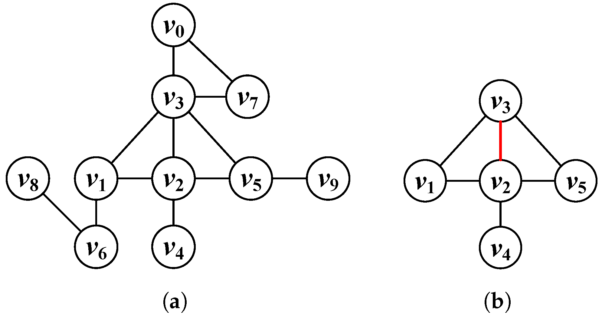
• Problem Statement. Given an undirected and unlabeled graph G(V, E) and its anonymized form G^*(V^*, E^*), it is essential to ensure that any attacker with background knowledge of 1-neighborhood information (i.e., degree or structural information) cannot re-identify any individual structural information through queries on G^*.

Definition 1

(Social network graph). An undirected, unlabeled graph $\mathit{G}(\mathit{V},\mathit{E})$, where $\mathit{V}$ represents the set of nodes (users) in the social network, $\mathit{E}$ represents the set of edges (relationships between users), and each $({\mathit{v}}_i,{\mathit{v}}_j)\in \mathit{E}$ represents the edge between ${\mathit{v}}_i\in \mathit{V}$ and ${\mathit{v}}_j\in \mathit{V}$.

Publishing the original graph G without proper anonymization can result in significant privacy risks for users. To mitigate these risks, the graph is typically anonymized before publication, with the k-anonymity method being one of the most widely used approaches.

Definition 2

(k-anonymity). Given a graph $G(V,E)$, the graph is k-anonymous if for each node $v\in V$, it is indistinguishable from at least $k-1$ other nodes.

k-anonymity is commonly used to protect users’ identities by modifying nodes so that each user is indistinguishable from $k-1$ other users. However, adversaries may use additional information, such as 1-neighborhood knowledge, to re-identify target nodes. Therefore, it is also necessary to protect the neighborhood information.

Definition 3

(1-neighborhood subgraphs [16]). Given a graph $G(V,E)$, $g\left(v\right)=⟨V\left(g\right(v\left)\right)$, and $E\left(g\right(v\left)\right)⟩$ represents the 1-neighborhood subgraph of v in the graph G, where $V\left(g\right(v\left)\right)$ represents the nodes connected to v within 1-hop distance in G, denoted as $V\left(g\right(v\left)\right)=\{u\mid (u,v)\in E\}\cup \left\{v\right\}$; $E\left(g\right(v\left)\right)$ represents the set of edges between nodes in $V\left(g\right(v\left)\right)$, denoted as $E\left(g\right(v\left)\right)=\left\{\right(u,v)\mid u,v\in V(g\left(v\right))\wedge (u,v)\in E\}$.

To address the limitations of k-anonymity, we introduce k-neighborhood subgraph anonymity and other anonymity methods.

Definition 4

(k-neighborhood subgraph anonymity). A graph $G(V,E)$ satisfies k-neighborhood subgraph anonymity if for each node $v\in V$, there are at least $k-1$ other nodes in V that have the same 1-neighborhood subgraph as v.

Definition 5

(Graph isomorphism [33]). Given two graphs $G(V,E)$ and $G^{*}(V^{*},E^{*})$, where $\left|V\right|=|V^{*}|$, G and $G^{*}$ are isomorphic if there exists a bijection h between V and $V^{*}$, $h:V\left(G\right)\to V\left(G^{*}\right)$, such that $(u,v)\in E$ if and only if $(h\left(u\right),h\left(v\right))\in E\left(G^{*}\right)$; then, G and $G^{*}$ are isomorphic. It is also said that there exists an isomorphism from G to $G^{*}$, or $(u,v)$ is isomorphic to $\left(h\right(u),h(v\left)\right)$.

Definition 6

(Partial isomorphism [35]). Given two graphs $G(V,E)$ and $G^{*}(V^{*},E^{*})$, and their subgraph structures A and B, G and $G^{*}$ are partially isomorphic if there exists a partial function, which is also a bijective function, $s:A\to B$, such that the relationship between the nodes in A is preserved and reflected in B when a node in A is mapped to B.

Definition 7

(k-isomorphism [33]). Given a graph $G(V,E)$, G satisfies the k-isomorphism if G consists of k disjoint subgraphs, i.e., $G=\{g_1,g_2,\dots ,g_k\}$, and these k subgraphs are isomorphic to each other.

4. TC$\mathit{\alpha }$-PIA

This paper proposes a novel tree clustering and $\alpha$-partial isomorphism anonymization scheme (TC$\alpha$-PIA) that satisfies different privacy requirements of users in the social network, effectively resists 1-neighborhood subgraph attacks, and preserves high utility of the anonymized graph.

As shown in Figure 1, the main process of TC$\alpha$-PIA includes the following steps: (1) Cluster nodes as multiple groups using the proposed similarity tree method. (2) Reduce inter-cluster differences using the proposed branch unification method. (3) Perform $\alpha$-partial isomorphism anonymization on the clustered groups to generate the anonymized graph.

Figure 1. An overview of TC$\alpha$-PIA.

4.1. Node Clustering Based on Similarity Tree

This section proposes a clustering method by constructing the similarity tree. This method groups similar nodes into multiple clusters, denoted as $\mathcal{C}=\{{\mathcal{C}}_1,{\mathcal{C}}_2,\dots ,{\mathcal{C}}_T\}$, where T is the number of clusters. In Algorithm 1, the process is divided into three main steps. First, we compute the similarity between each pair of nodes (lines 1–15). Second, we construct a similarity tree based on the similarity results (lines 16–26). Finally, we perform branch unification on the constructed similarity tree to minimize inter-cluster differences (line 27). The details are as follows.

Algorithm 1 Similarity tree established

Require: Original graph $G(V,E)$, anonymity parameter k, number of nodes n Ensure: Number of clusters C, ordered similarity list D, similarity tree $Tree$ 1: for $i=1$ to n do 2:       Compute ${\mathit{x}}_i=<d_i,E_{g_i},{\Delta }_i,O{E}_{{\Delta }_i}>$ for each node 3: end for 4: $m=0$ 5: for $i=1$ to n do 6:       for $j=i+1$ to n do 7:             Calculate the similarity of each node 1-neighborhood graph 8:       end for 9:       $M=$ Sort Based on Similarity 10:     for $z=1$ to n do 11:           $D(m,0)=M(z-1,0)$ 12:           $D(m,1)=M(z-1,1)$ 13:           $m=m+1$ 14:     end for 15: end for 16: $m=0$, $Tree\leftarrow \mathrm{null}$, $\mathit{Tree}.\mathit{root}\leftarrow \mathrm{null}$ 17: for $i=1$ to n do 18:       $v_i.parent\leftarrow D(m,1)$ 19:       $v_i.parent.children\leftarrow v_i$ 20:       $m=m+n$ 21: end for 22: for $i=1$ to n do 23:       if $v_i.parent$ is null then 24:            $v_i.parent\leftarrow Tree.root$ 25:       end if 26: end for 27: Branch Unification seeing Algorithm 2 return C, D, $Tree$

Step 1: node similarity calculation. The similarity between each pair of nodes is calculated by the combined criterion, which includes four factors: the node’s degree, the number of edges in the 1-neighborhood subgraph of the node, the number of triangles in which the node participates (triangles involving the node), and the number of common edges of triangles in which the node participates (overlapping edge of participating triangles). The latter two factors are further given as follows:

Definition 8

(Triangles involving the node). An undirected and unlabeled original graph $G(V,E)$, where $V=V\left(G\right)$ is the set of nodes and $E=E\left(G\right)$ is the set of edges. The triangles involving the node v are defined as $\Delta \left(v\right)=\{v\mid z\in V\wedge u\in V\wedge (u,v)\in E(G)\wedge (v,z)\in E(G)\wedge (u,z)\in E(G\left)\right\}$, where u, v, and z are nodes in G. For example, Figure 2a is the 1-neighborhood subgraph of $v_2$. It contains two triangles: one comprises $v_1$, $v_2$, and $v_3$, and the other comprises $v_2$, $v_3$, and $v_5$. For ease of understanding, we will use the term “participating triangle” in the following.

Figure 2. Example of triangles involving the node: (a) Original graph. (b) The 1-neighborhood subgraph of $v_2$ containing two participating triangles $(v_1,v_2,v_3)$ and $(v_2,v_3,v_5)$ and one overlapping edge $(v_2,v_3)$.

Definition 9

(Overlapping edge of participating triangles). An undirected, unlabeled graph $G(V,E)$, where V is the set of nodes and E is the set of edges. We define the common edge between several participating triangles in Definition 10 as the overlapping edge of the participating triangles: $OE=\{(u,v)\mid u,v\in V\wedge (u,v)\in E\left({\Delta }_1\right)\cap E\left({\Delta }_2\right)\wedge E\left({\Delta }_1\right),E\left({\Delta }_2\right)\in E\}.$ For example, the red line in Figure 2b is the common edge between the above two triangles.

Then, we give the formula of similarity calculation based on the four factors mentioned above.

$$\Delta f=∥{\mathit{x}}_i-{\mathit{x}}_j∥.$$

(1)

$${\mathit{x}}_i=<d_i,E_{g_i},{\Delta }_i,O{E}_{{\Delta }_i}>.$$

(2)

where $\Delta f$ is the similarity function, and the smaller its result, the higher the similarity between two nodes. ${\mathit{x}}_i$ is a vector about the node $v_i$, and it includes four factors: $d_i$, $E_{g_i}$, ${\Delta }_i$, and $O{E}_{{\Delta }_i}$. $d_i$ is the node’s degree, $E_{g_i}$ is the number of edges in the 1-neighborhood subgraph $g_i$ of the node, ${\Delta }_i$ represents the triangles involving the node, and $O{E}_{{\Delta }_i}$ is the overlapping edge of participating triangles. The last two factors, ${\Delta }_i$ and $O{E}_{{\Delta }_i}$, account for the stability of the triangle structures and the number of participating paths, thus better capturing the 1-neighborhood subgraph structure.

After calculating the similarity, the results are stored in a list $\mathit{D}$ of size $n\times 2$. $\mathit{D}(i,0)$ stores the similarity values between $v_i$ and other nodes in ascending order, denoted as $Sim\left(v_i\right)=\{Sim(v_i,v_j)\mid i,j=1,2,\dots ,n-1\mathrm{and}i\ne j\}$. $\mathit{D}(i,1)$ stores the corresponding nodes in the order of $Sim\left(v_i\right)$, denoted as $PN\left(v_i\right)=\{v_j\mid j=1,2,\dots ,n-1\}$.    

$$\mathit{D}=\left(\begin{array}{cc}sim\left(v_1\right)& PN\left(v_1\right)\\ sim\left(v_2\right)& PN\left(v_2\right)\\ ⋮& ⋮\\ sim\left(v_n\right)& PN\left(v_n\right)\end{array}\right)$$

Step 2: similarity tree construction. To ensure tight connections within clusters, we construct a similarity tree based on the calculated similarities. Each node is connected to its most similar node, referred to as the parent node, forming the branches of the tree. For nodes that are most similar but not identical, such as $v_2$ and $v_6$ in Table 1, one node is randomly chosen as the parent and the other as the child to form the relationship tree. Nodes without a parent node are connected directly to the root node, which is used only for tree construction and does not correspond to an actual node in the graph, nor does it participate in the clustering process. Each branch under the root node represents a cluster. The relevant definitions are as follows:

Table 1. Example of parent–child node relationship.

$v_i$	$v_1$	$v_2$	$v_3$	$v_4$	$v_5$	$v_6$	$v_7$	$v_8$	$v_9$
$P\left(v_i\right)$	$v_5$	$v_6$ (root)	$v_5$ (root)	$v_6$	$v_3$	$v_2$	$v_6$	$v_7$	$v_8$

Definition 10

(Parent–child node relationship). For each $v_i$, identify the $v_j$ that is most similar to $v_i$ by selecting the first element in $PN\left(v_i\right)$, denoted as $P\left(v_i\right)=PN\left(v_i\right)\left[1\right]$, where $P\left(v_i\right)$ is the parent node of $v_i$.

Table 1 and Figure 3 show the establishment of parent–child relationships and the construction process of the similarity tree, respectively. Each node is directly connected to its parent node, $P\left(v_i\right)$. For example, both $v_7$ and $v_4$ have the same parent node, $v_6$, and are directly connected to it. In cases where nodes are most similar, such as $v_2$ and $v_6$, one node is randomly selected as the parent. Here, $v_2$ is chosen as the parent of $v_6$; similarly, the relationship between $v_3$ and $v_5$ is established in the same manner. Consequently, we obtain two branches in Figure 3a: $\{v_2,v_6,v_7,v_4,v_8,v_9\}$ and $\{v_3,v_5,v_1\}$. From Figure 3a, it is clear that $v_2$ and $v_3$ do not have parent nodes. For such nodes, we directly connect them to the root node; i.e., $v_2$ and $v_3$ are connected directly to the root node, as indicated by the text “root” in Table 1.

Figure 3. Example of similarity tree construction (setting k = 3): (a) Two branches, $\{v_2,v_6,v_7,v_4,v_8,v_9\}$ and $\{v_3,v_5,v_1\}$, where $v_2$ and $v_3$ have no parent nodes. (b) Connect the nodes $v_2$ and $v_3$ to the root node. (c) After branch unification, we obtain three independent branches, corresponding to three clusters: $C_1=\{v_7,v_8,v_9\}$, $C_2=\{v_2,v_6,v_4\}$, and $C_3=\{v_3,v_5,v_1\}$.

Step 3: branch unification of the similarity tree. The varying branch sizes in the similarity tree can cause differences in anonymity levels and increase the risk of information leakage. We unified branches of the similarity tree, ensuring that all clusters were of the same size. As shown in Figure 3b,c, when $k=3$, we split the branches that contained significantly more than three nodes. Starting from the bottom, we divided $v_9,v_8,$ and $v_7$ from the branch to form an independent branch and connected it to the root node.

Algorithm 2 presents the details for the branch unification of the similarity tree. The key steps are as follows: (1) Traverse each branch of the similarity tree and perform removal or splitting operations on nodes within the branches (lines 2–10) to achieve a unified number of nodes among branches. The quality of clustering is ensured by rationalizing and reassigning nodes and tree branches. (2) Mark branches with more than k nodes and those with significantly fewer than $\sqrt{k}$ nodes. Remove the excess nodes from branches with more than k nodes and eliminate branches with fewer nodes than $\sqrt{k}$. Based on the similarity results, reassign the removed nodes to the next-most-similar parent node as sub-nodes of that node (lines 11–19). (3) To maintain clustering quality, check the number of neighbors for the nodes within each branch. Remove nodes with significant differences in similarity and reassign them to the next-most-similar node (lines 20–26).

Algorithm 2 Branch unification

Require: k, D, tree root $Tree\_root$ Ensure: C, $Tree$ 1: $S\leftarrow \varnothing$, $Tree\_root\leftarrow root$ 2: for branch in root.children do         ▹ Iterate through branches under the root node 3:        if $\left|\mathrm{branch}\right|\ll \sqrt{k}$ then 4:              Remove the branch from root and add nodes from the branch to S 5:        else if $\left|\mathrm{branch}\right|>k$ then 6:              Place the remaining $|\mathrm{branch}\%k|$ in S 7:              $R_{bi}\leftarrow$ Divide branch into equal branches 8:              Add $R_{bi}$ into $root.children$       ▹ Split the branch and connect to the root node 9:        end if 10: end for 11: while S not empty do               ▹ Search for the next parent for the removed nodes 12:       for $i=1$ to $\left|S\right|$ do 13:              Find next parent node $p_{v_i}$ from D 14:              if $\left|\mathrm{branch}\right(p_{v_i}\left)\right|\le k$ then 15:                    $v_i.\mathrm{parent}\leftarrow p_{v_i}$ 16:                    Remove $v_i$ from S 17:              end if 18:       end for 19: end while 20: $S\leftarrow \varnothing$ 21: for $branch$ in $root.children$ do 22:       Remove nodes with significant differences 23:       Add nodes to S 24: end for 25: Repeat steps 12–19 until S is empty 26: Update $Tree$, $C\leftarrow \mathrm{branches}$ return C, $Tree$

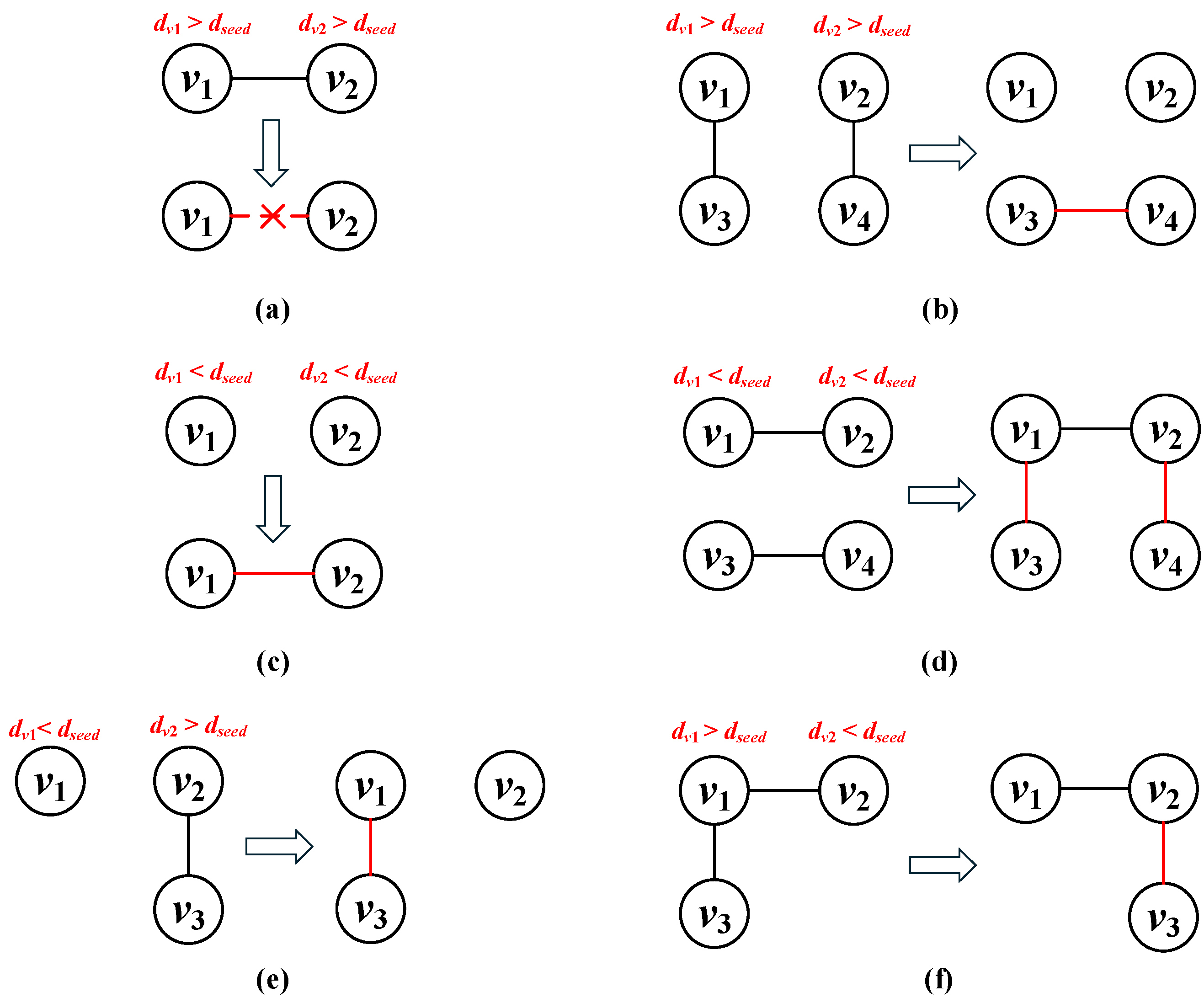
4.2. Graph Anonymity Modification Based on $\alpha$-Partial Isomorphism

After clustering nodes, this section anonymizes nodes within each cluster using the proposed $\alpha$-partial isomorphism. This method includes the following steps: (1) Select seed nodes and determine $\alpha$ values for each cluster. (2) Establish the mapping relationship between the 1-neighborhood graph of the node and the 1-neighborhood graph of the seed node in each cluster. (3) Based on the mapping relationship, establish a mapping matrix between the nodes and their corresponding seed nodes. Compare the structural information in the matrix and calculate the percentage of identical structures. Then, compare this proportion with the $\alpha$ value and perform the necessary anonymization modifications based on the requirements. We first give the relevant definitions before presenting the $\alpha$-partial isomorphism algorithm.

Definition 11

(Mapping relationship). Given a graph $G(V,E)$, where $g\left(v\right)$ and $g\left(u\right)$ are 1-neighborhood subgraphs of nodes v and u in G., if there is a correspondence between nodes in $g\left(v\right)$ and $g\left(u\right)$, then there is mapping between $g\left(v\right)$ and $g\left(u\right)$, denoted as $f:g\left(v\right)\to g\left(u\right)$. Figure 4 and Table 2 show an example of a mapping relationship.

Figure 4. Mapping relationship.

Table 2. Subgraph node sequence and mapping relationship.

${\mathit{g}}_{\mathit{i}}$	Degree_Sequence	Map<${\mathit{g}}_1,{\mathit{g}}_2$>
$g_1$	4, 3, 2, 2, 1	(1, 8), (3, 6), (2, 7), (4, 0), (5, 9)
$g_2$	4, 2, 2, 2, 2

Definition 12

(Centrality of edge neighborhood [23]). The neighborhood centrality of an edge is used to measure the importance or centrality of an edge in a network, which describes the influence of an edge $(v_i,v_j)$ in its neighborhood and can be expressed by the following equation:

$$NC\{v_i,v_j\}={\displaystyle \frac{|\mathrm{\Gamma }\left(v_i\right)\cup \mathrm{\Gamma }\left(v_j\right)|-|\mathrm{\Gamma }\left(v_i\right)\cap \mathrm{\Gamma }\left(v_j\right)|}{2max\left(deg\right)}}.$$

(3)

where $NC$ represents the neighborhood centrality of the edge $(v_i,v_j)$, and $\mathrm{\Gamma }\left(v_i\right)$ denotes the number of neighbors of node $v_i$. Since the edges between two nodes are removed randomly, there is a risk of destroying the triangles in the graph. Therefore, based on the above definition, this paper uses the edge participation measure mentioned in Definition 11 to minimize the effect on the triangle structure. The calculation is as follows:

$$NC\_remove(v_i,v_j)=NC(v_i,v_j)\times (r_{{\Delta }_{g_i}}+1)$$

(4)

where $NC\_remove$($v_i$, $v_j$) is the edge to be removed.

Figure 5 provides an example to illustrate the process of $\alpha$-partial isomorphism anonymization based on the above definitions. (1) First, the seed node, highlighted in red, is selected as the node with the largest number of neighbors in each cluster. Simultaneously, the maximum $\alpha$ value for each cluster is determined and labeled as ${\alpha }_i$ ($i=1,2,3,4$), also highlighted in red in Figure 5. (2) Next, we establish the mapping relationship between the 1-neighborhood graph of each node and the 1-neighborhood graph of the seed node in descending order by node degree within each cluster, and establish mapping matrices $\mathit{MD}$. For illustration, we use cluster $C_2$, which contains nodes $v_2$ and $v_3$, with a similar process applied to other clusters. We calculate the percentage of identical structures between nodes $v_2$ and $v_3$ by comparing the common edges in the $\mathit{MD}$, where $\mathit{MD}$[i][j] = 1 indicates the presence of an edge between the two nodes and $\mathit{MD}$[i][j] = 0 indicates its absence. Although $v_2$ and $v_3$ have the same 1-neighborhood structure with six identical edges, the unequal number of neighbors means that ${\alpha }_2$ (100%)-partial isomorphism is not satisfied. To achieve structural isomorphism with the seed node $v_2$, a fake node $f_1$ is added and connected to $v_3$. (3) After modifications within all clusters, the fake nodes are merged to avoid the excessive addition of fake nodes, as shown in Figure 5. Merging $f_1$ and $f_2$ is effective because it does not compromise the privacy of nodes $v_3$ and $v_8$.

Figure 5. $\alpha$-partial isomorphism: (a) Original graph G. (b) Select the seed node with the largest number of neighbors and maximum ${\alpha }_i$ value in each cluster. (c) Establish the mapping relationship between the 1-neighborhood subgraph of a node and the 1-neighborhood subgraph of the seed node in each cluster. (d) Modify the 1-neighborhood subgraph structure of a node to achieve ${\alpha }_i$-partial isomorphism by referencing the 1-neighborhood structure of the seed node. (e) Anonymized graph $G^{\sim }$. (f) Merge the fake nodes to obtain the final anonymized graph $G^{*}$.

Algorithm 3 presents a detailed description of graph anonymity based on $\alpha$-partial isomorphism anonymization. (1) First, the node with the largest number of neighbors in each cluster is selected as the seed node, and the maximum value of ${\alpha }_i$ is determined for each cluster $C_i$ (lines 1–3). The selection of ${\alpha }_i$ is based on the privacy threshold specified by the users. The privacy requirements of the users are classified into three levels, strong, medium, and weak, corresponding to the intervals [0%, 30%], (30%, 60%], and (60%, 100%], respectively. ${\alpha }_i$ is determined by identifying the highest privacy requirement within each cluster. For example, if the privacy requirements of three users in cluster $C_i$ are 25%, 52%, and 20%, then ${\alpha }_1$ is set to 52% for $C_i$, indicating a medium privacy requirement. (2) Second, after selecting the seed node and max ${\alpha }_i$ in each cluster, we use the mapping matrix to evaluate the structural similarity between the seed node and other nodes. If the similarity meets the threshold ${\alpha }_i$, these nodes are considered isomorphic to the seed node and require no further anonymization. Otherwise, we adjust their 1-neighborhood subgraph structures until ${\alpha }_i$ is reached (lines 4–37). (3) Third, since the anonymization process described in Step 2 may involve the addition of fake nodes, we propose a node-merging strategy. This strategy evaluates pairs of fake nodes to determine whether they can be merged without compromising the privacy of the connected nodes. If merging fake nodes changes their 1-neighborhood structure and does not satisfy the ${\alpha }_i$ structure anonymity requirements for the connected nodes, then the fake nodes should not be merged. This approach ensures privacy while optimizing the graph structure and minimizing the disruption caused by the addition of fake nodes (lines 38–42).

Algorithm 3 Graph anonymity

Require: $G(V,E)$, Structure level anonymity threshold $\alpha$ Ensure: Anonymized graph $G^{*}$ 1: for $i=1$ to C do 2:       Find seed node in $C_i$ 3:       determine the maximum ${\alpha }_i$ value in $C_i$ 4:       for node in $C_i$ do 5:              if $\mathrm{sim}(\mathrm{node},\mathrm{seed})<{\alpha }_i$ then 6:                    Add $(d_{\mathrm{seed}}-d_{\mathrm{node}})$ fake nodes into $g_{\mathrm{node}}$ 7:                    Sort the nodes in subgraph $(g_{\mathrm{seed}},g_{\mathrm{node}})$ according to degree 8:                    $M_p(g_{\mathrm{seed}},g_{\mathrm{node}})\leftarrow$ Mapping node in seed node 9:                    $MD(g_{\mathrm{seed}},g_{\mathrm{node}})\leftarrow$ Mapping matrix 10:                   $S_1\leftarrow \varnothing$, $S_2\leftarrow \varnothing$ 11:                   for v in $g_{\mathrm{node}}$ do 12:                         if $d_v<d_{M_p(v,\mathrm{seed})}$ then 13:                               Add v into $S_1$ 14:                         else if $d_v>d_{M_p(v,\mathrm{seed})}$ then 15:                               Add v into $S_2$ 16:                         end if 17:                   end for 18:                   for $v_1,v_2$ in $S_1$ do 19:                         Add the edge($v_1,v_2$) 20:                   end for 21:                   for $v_1,v_2$ in $S_2$ do 22:                         if $d_{v_1}>d_{M_p(v_1,\mathrm{seed})}$ and $v_2\in g_{v_1}$ and $min\left\{N{C}_{\mathrm{remove}}(v_1,v_2)\right\}$ then 23:                               Remove the edge($v_1,v_2$) 24:                         end if 25:                   end for 26:                   Update $S_1,S_2$ 27:                   if $\mathrm{sim}(\mathrm{node},\mathrm{seed})<{\alpha }_i$ then 28:                         Matching triangle structures with $MD(g_{\mathrm{seed}},g_{\mathrm{node}})$ 29:                         Repeat similar steps 6–27 30:                         if $\mathrm{sim}(\mathrm{node},\mathrm{seed})<{\alpha }_i$ then 31:                               Modify edges using $MD$ 32:                         end if 33:                         Repeat until $\mathrm{sim}(\mathrm{node},\mathrm{seed})\ge {\alpha }_i$ 34:                   end if 35:              end if 36:       end for 37: end for 38: for each fake node pair $(f_1,f_2)$ do 39:     if No node privacy is compromised by merging $f_1$ and $f_2$ then 40:           Merge fake nodes $f_1$ and $f_2$ 41:     end if 42: end for return  $G^{*}$

Figure 6 shows examples of edge addition and deletion in the Algorithm 3, covering cases not illustrated in Figure 5.

Figure 6. Edge modification strategy: (a) A degree reduction/edge deletion strategy for when there is an edge between $v_1$ and $v_2$. (b) A degree reduction/edge deletion strategy for when there is no edge between $v_1$ and $v_2$. (c) A degree increase/edge addition strategy for when there is no edge between $v_1$ and $v_2$. (d) A degree increase/edge addition strategy for when there is an edge between $v_1$ and $v_2$. (e) An edge swapping strategy for when there is no edge between $v_1$ and $v_2$. (f) An edge swapping strategy for when there is an edge between $v_1$ and $v_2$.

(1) Both $v_1$ and $v_2$ need to decrease their degrees. If there is an edge between $v_1$ and $v_2$, delete the edge between the two nodes. If there is no edge between $v_1$ and $v_2$, use Formulas (3) and (4) to find and delete the edge with the least effect. To ensure the degrees of $v_3$ and $v_4$ remain unchanged, add an edge between them.

(2) Both $v_1$ and $v_2$ need to increase their degrees. If there is no edge between $v_1$ and $v_2$, add one. If an edge already exists between $v_1$ and $v_2$, find non-adjacent nodes for $v_1$ and $v_2$, and connect them to $v_1$ and $v_2$, respectively. To maintain the original degrees, the existing edge between the newly connected nodes should be removed. For example, connect $v_3$ to $v_1$ and $v_2$ to $v_4$, while removing the edge between $v_4$ and $v_3$.

(3) $v_1$ needs to increase its degree, while $v_2$ needs to decrease its degree. We use Formulas (3) and (4) to remove the edge with the lowest centrality in $v_2$’s neighborhood and reconnect the disconnected node to $v_1$. This adjustment does not affect the degree of the node previously connected to $v_2$, while satisfying the requirement for increasing the degree of $v_1$ and decreasing the degree of $v_2$.

(4) $v_1$ needs to decrease its degree, while $v_2$ needs to increase its degree. This process is analogous to (3), so a detailed explanation is omitted here.

4.3. Algorithm Complexity Analysis

According to the previous chapters, TC$\alpha$-PIA mainly includes node clustering based on the similarity tree and anonymous graph modification based on $\alpha$-partial isomorphism anonymization.

In the node clustering phase, the complexity of similarity calculation is $O\left(n^2\right)$, where n is the number of nodes. The complexity of similarity tree construction is $O\left(n\right)$. In the branch unification of the similarity tree, nodes and branches not meeting the requirements are removed, with a complexity of $O\left(l\right)$, where l is the number of branches. The complexity for reallocating these removed nodes and branches has two cases. In the best case, each excluded node can easily find its parent node, and the branch of the parent node can continue to accommodate its child nodes. The complexity is $O\left(m\right)$, where m is the number of nodes removed from the branches. In the worst case, the parent node’s branch cannot accommodate new nodes, and the excluded node must continuously search for the parent node. The complexity is $O(m·n)$. In summary, the best-case complexity of branch unification for the similarity tree is $O(n^2+n+l+m)$, and the worst-case complexity is $O(n^2+n+l+m·n)$. Since $l,m\ll n$, the overall complexity of the clustering process is approximately $O\left(n^2\right)$.

In the graph-anonymization phase, each cluster is searched for the seed node and $\alpha$, with a time complexity of $O\left(\right|C\left|\right)$, where $\left|C\right|$ represents the number of clusters identified after branch unification. The complexity of node anonymization in each cluster is $O\left(\right|C_i|·d)$, where $|C_i|$ denotes the number of nodes in the cluster and d represents the average degree difference between nodes requiring modification to achieve partial $\alpha$-partial isomorphism with the seed node.

In summary, the time complexity of TC$\alpha$-PIA is $O(n^2+|C|·|C_i|·d)$.

4.4. Privacy Analysis

In this section, we demonstrate the effectiveness of TC$\alpha$-PIA for anonymizing the social network graph structure while satisfying users’ different privacy requirements. The anonymized graph obtained by the TC$\alpha$-PIA scheme can resist attacks from adversaries with different background knowledge.

Theorem 1.

For the complete or partial 1-neighborhood graph attack of any target node, the probability that the attacker can re-identify the target node’s identity does not exceed 1/k.

Proof of Theorem 1.

Assume there exist two kinds of attacks according to the capability of the attacker: (1) The attacker has partial knowledge of the 1-neighbor subgraph of the target node. (2) The attacker has complete knowledge of the 1-neighbor subgraph of the target node.

Partial protection analysis. The attacker has a partial 1-neighbor subgraph structure of the target node. In this scenario, the attacker’s matching results may be biased, and cannot be guaranteed to fully match the corresponding node clusters. In addition, it can be guaranteed that at least $k-1$ nodes have a 1-neighbor subgraph identical to that of the target node. Therefore, the probability that the attacker can uniquely identify the target node is not higher than $1/k$.

Complete protection analysis. The attacker has completed the 1-neighbor subgraph structure of the target node. Since our scheme allows subgraphs to be isomorphic, at least $k-1$ nodes will have the same 1-neighborhood subgraph as the target node. Therefore, TC$\alpha$-PIA satisfies the anonymity requirement; i.e., the probability that the attacker can uniquely identify the target node is no higher than $1/k$. □

5. Experimental Evaluations

In Section 5.1, we introduce the datasets used in the experiments. In Section 5.2, we describe the metrics used to evaluate the experimental results. In Section 5.3, we explore the performance of TC$\alpha$-PIA and the comparative experiment.

5.1. Datasets

Four real datasets are used in our experiments, and their statistics are shown in Table 3.

Table 3. Real-world graph datasets.

Dataset	$\left|\mathit{N}\right|$	$\left|\mathit{E}\right|$	AVD	ACC	APL
Facebook	4039	88,234	44	0.605	4.7
CA-CondMat	23,133	186,936	8	0.633	6.4
email-Eu-core	986	24,929	32.58	0.407	2.587
soc-wiki-Vote	889	2914	6.56	0.153	4.096

• The Facebook dataset [36] from SNAP, with 4039 nodes representing users and 88,234 edges representing relationships.
• The Ca-CondMat dataset [36] on condensed matter physics, with 23,133 nodes representing papers and 186,936 edges representing co-authorship.
• The email-Eu-core dataset [36], with 986 nodes representing users and 25,571 edges representing email communications.
• The soc-wiki-Vote dataset [37], with 889 nodes representing Wikipedia users and 2916 edges representing voting interactions.

5.2. Utility Metrics

To evaluate the proposed TC$\alpha$-PIA scheme, we used the following metrics:

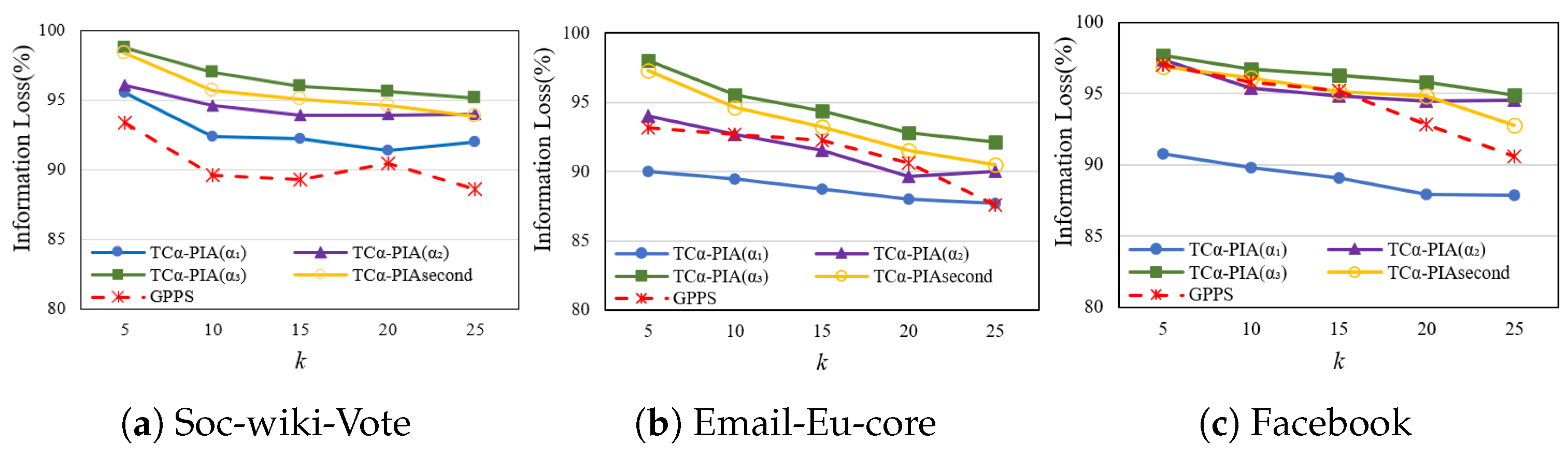
• Information Loss (IL). IL refers to the data difference between the modified graph and the original graph after modifications. Modifications include adding or deleting nodes and edges, and edge swapping, which can cause information loss in the original graph. The formula for calculating the information loss [13] is as follows.

  $$IL=\delta ·ND(G,G^{*})+(1-\delta )·ED(G,G^{*})$$

  (5)

  where

  $$ND={\displaystyle \frac{1}{2}}·({\displaystyle \frac{|N\left(G\right)\cap N\left(G^{*}\right)|}{\left|N\right(G\left)\right|}}+{\displaystyle \frac{|N\left(G\right)\cap N\left(G^{*}\right)|}{\left|N\right(G^{*}\left)\right|}})$$

  (6)

  $$ED={\displaystyle \frac{1}{2}}·({\displaystyle \frac{|E\left(G\right)\cap E\left(G^{*}\right)|}{\left|N\right(G\left)\right|}}+{\displaystyle \frac{|E\left(G\right)\cap E\left(G^{*}\right)|}{\left|N\right(G^{*}\left)\right|}})$$

  (7)

  where $ED$ represents the information loss of edges, $ND$ represents the information loss of nodes, $E\left(G\right)$ represents the edges of the original graph, $E\left(G^{*}\right)$ represents the edges of the anonymized graph, and $ND\left(G\right)$ and $ND\left(G^{*}\right)$ represent the nodes in the original and anonymized graphs, respectively. $\delta$ represents the weight parameter, with a value range of [0,1]. The above formula can calculate different results based on the different emphases of the anonymity scheme on nodes and edges in the graph. In general, the larger the calculated result, the higher the degree of information preservation from the original graph.
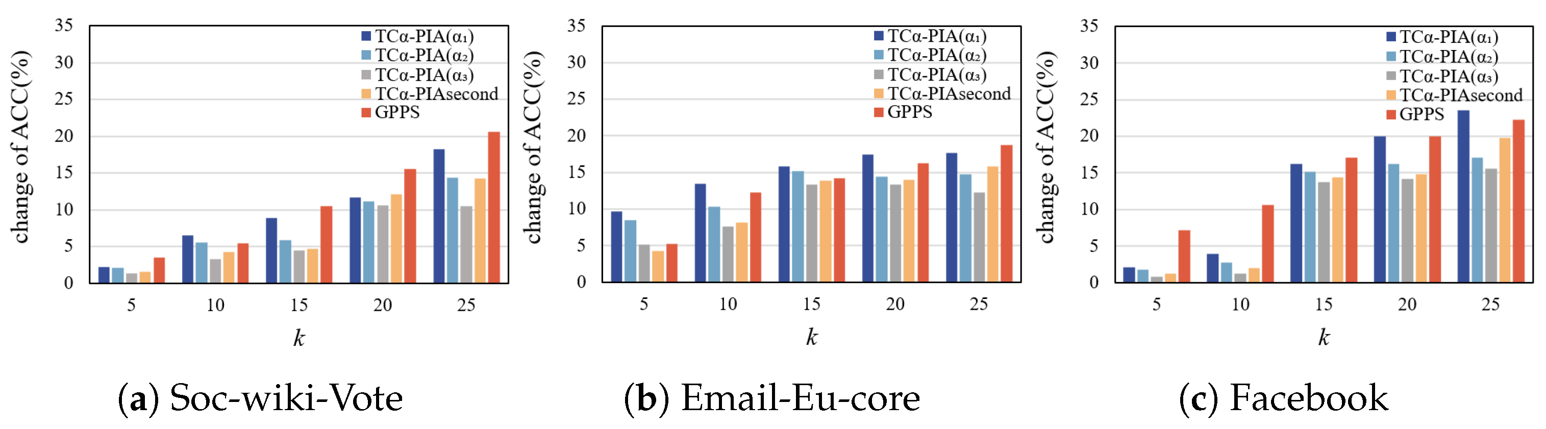
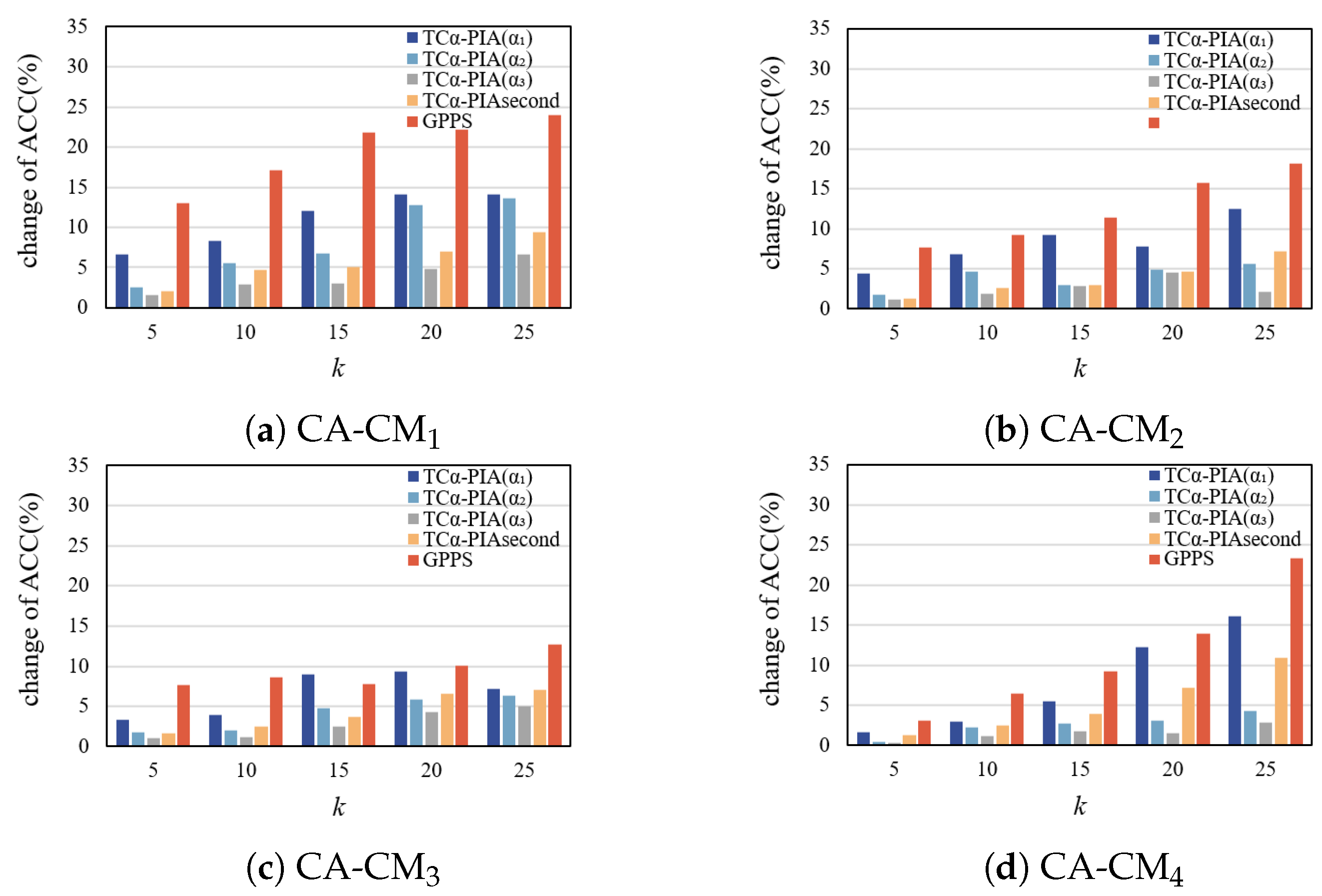
• Average Clustering Coefficient (ACC). ACC focuses on the closeness between nodes, that is, the number of connections between nodes. The change in ACC can reveal the degree of change in the connection relationship between nodes in the graph after anonymization.

  $$ACC={\displaystyle \frac{1}{\left|N\right|}}\sum _{i=1}^{\left|N\right|}{C}_i$$

  (8)

  where $\left|N\right|$ is the number of nodes in the graph and $C_i$ is the local clustering coefficient of node i.
• Average Shortest Path Length (APL). The average shortest path length is the average length of the shortest path between any two nodes in the graph. By comparing the average shortest path length of the original and anonymous graphs, we can understand the influence of anonymization on graph connectivity.

  $$APL={\displaystyle \frac{{\sum }_{i\ne j}path(v_i,v_j)}{\left|N\right|\left(\right|N|-1)}}$$

  (9)

  where $path(v_i,v_j)$ is the length of the shortest path between nodes $v_i$ and $v_j$.
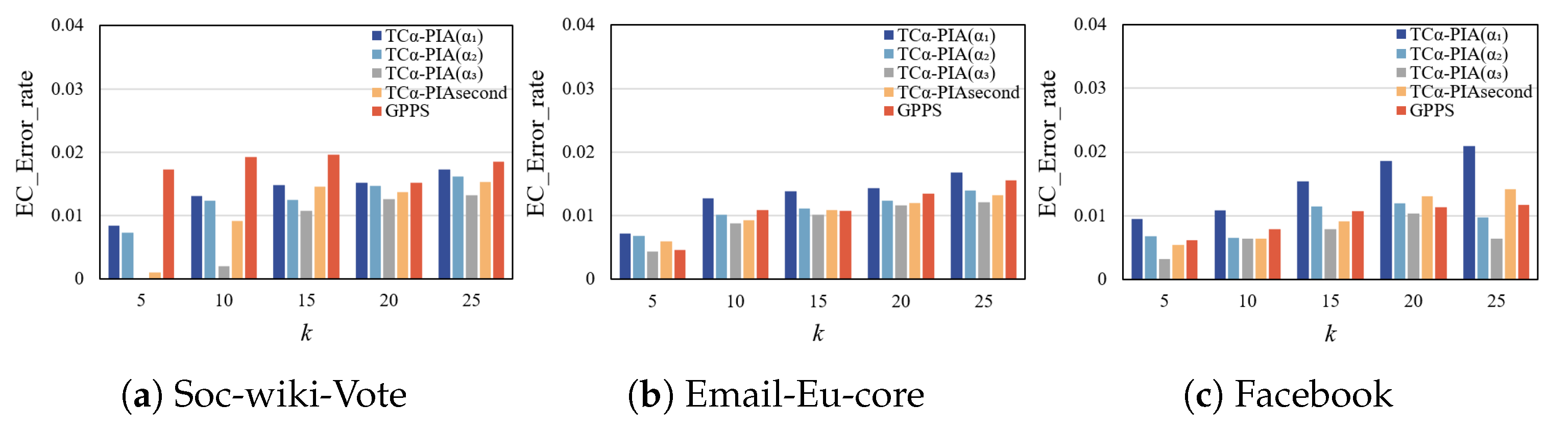
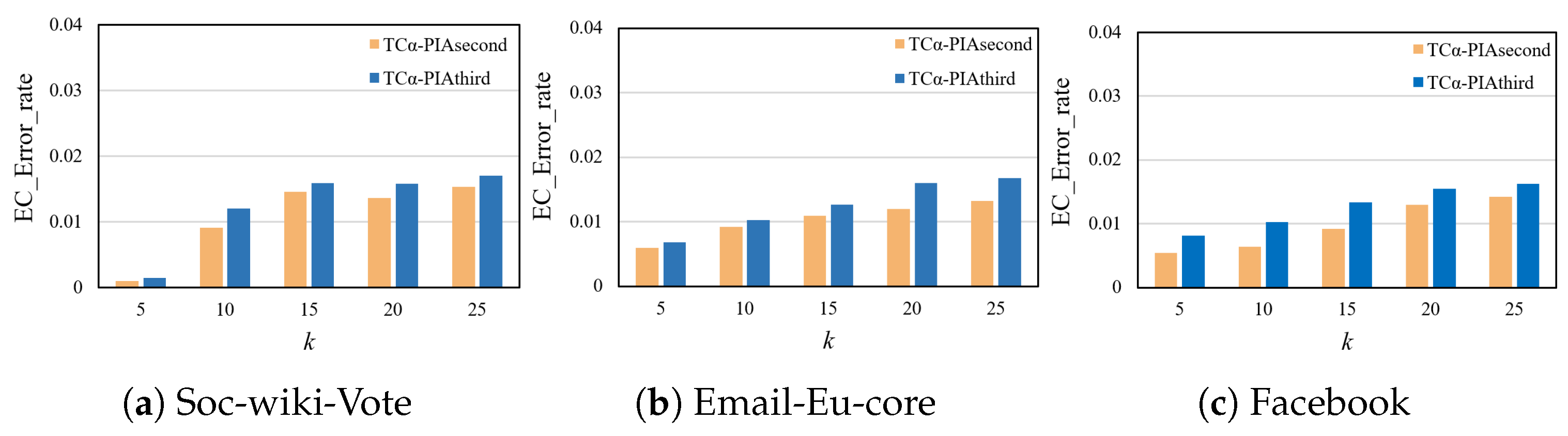
• Eigenvector Centrality (EC). Eigenvector centrality is used to measure the importance of nodes in a network structure. Analyzing the change in eigenvector centrality can provide insight into changes in the importance and influence of nodes caused by anonymization.

5.3. Comparison and Analysis of Experimental Results

Implementation. The experimental setup consists of a device manufactured by Lenovo located in Beijing, China, equipped with an AMD Ryzen 5 5600H processor with Radeon Graphics clocked at 3.30 GHz and 16 GB RAM. The operating system used is Windows 10 Home, and the programming language used for the implementation is Python 3.7.

Comparison. To demonstrate the effectiveness of our proposed TC$\alpha$-PIA scheme, we performed the following experimental comparisons: (1) We compared the TC$\alpha$-PIA scheme with the GPPS [16] introduced in Section 1. For a fair comparison, we used consistent $\alpha$ values for uniform anonymity and compared them with the GPPS scheme. In addition, we compared the results under different $\alpha$ values (referred to as TC$\alpha$-PIA_second), with those of the GPPS scheme. Note that the results of GPPS are averaged over several experiments under non-isomorphic conditions, while the TC$\alpha$-PIA_second results are the average of several experiments with different $\alpha$ values required by different users. (2) To validate the effectiveness of tree clustering based on the combined criterion, we compared it with traditional clustering based on Euclidean similarity within the same anonymity scheme.

Experimental settings. We set $k=5$, 10, 15, 20, 25. For TC$\alpha$-PIA, we set three $\alpha$ values: ${\alpha }_1=100\%$, ${\alpha }_2=50\%$, and ${\alpha }_3=10\%$.

5.3.1. Comparison of the Overall Performance of Schemes

This experiment was performed on both complete and random graphs. For random graphs, we followed the method in reference [13] and randomly extracted 500 to 2000 nodes and their edges from the larger Ca-CondMat dataset to construct four random graph datasets for further experimental comparison with the GPPS scheme [16]. These datasets are denoted as CA-CM₁, CA-CM₂, CA-CM₃, and CA-CM₄, respectively, and contain 500, 1000, 1500, and 2000 nodes and their corresponding edges.

Complete graphs

• Comparison of IL.

Figure 7a shows the effect of different schemes on the IL in the soc-wiki-Vote dataset. It is evident that as $\alpha$ decreases, the IL of TC$\alpha$-PIA increases, indicating fewer modifications to the original graph and better preservation of the original data. In addition, for the same $\alpha$, IL decreases as k increases, suggesting that higher privacy levels result in lower utility of the graph. The lower IL at $k=15$ compared to $k=20$ is due to dataset inhomogeneities causing experimental fluctuations. Compared to GPPS, TC$\alpha$-PIA(${\alpha }_1$), TC$\alpha$-PIA(${\alpha }_2$), and TC$\alpha$-PIA(${\alpha }_3$) perform better, as the proposed scheme effectively limits the addition of fake nodes and edges, reducing their impact on the original graph. Unlike TC$\alpha$-PIA, TC$\alpha$-PIA_second considers the different $\alpha$ requirements of all users. Since not all users require weak privacy, TC$\alpha$-PIA_second results in slightly lower IL compared to TC$\alpha$-PIA(${\alpha }_3$). However, it outperforms TC$\alpha$-PIA(${\alpha }_2$), TC$\alpha$-PIA(${\alpha }_1$), and GPPS by considering different privacy requirements, rather than applying a uniform $\alpha$. This reduces unnecessary modifications and makes anonymization more efficient, preserving more of the original graph structure.

Figure 7. Comparison of IL on complete graphs.

Figure 7b,c show the results for the Email-Eu-core and Facebook datasets, respectively. In Figure 7b, TC$\alpha$-PIA(${\alpha }_3$) significantly outperforms GPPS. For $k<20$, the IL of TC$\alpha$-PIA(${\alpha }_2$) is comparable to that of GPPS, while TC$\alpha$-PIA(${\alpha }_1$) performs slightly worse. The analysis for TC$\alpha$-PIA_second is consistent with the findings in Figure 7a.

Overall, TC$\alpha$-PIA performs better on the soc-wiki-Vote dataset, and all four TC$\alpha$-PIAs outperform GPPS with different parameters because they are better suited for uniformly distributed and moderately sized graph networks.

• Change in ACC.

Figure 8a shows the effect of different schemes on ACC in the soc-wiki-Vote dataset. TC$\alpha$-PIA consistently has a lower rate of change in ACC compared to GPPS, indicating better performance. This result is attributed to the fact that TC$\alpha$-PIA considers the triangle structure and number during structural anonymization, which helps to preserve more original edges and structures. As k increases, the impact of each scheme on the ACC gradually increases, i.e., the difference between the anonymized graph and the original graph increases. This is because higher anonymity levels lead to more changes in the graph. In the TC$\alpha$-PIA scheme, a smaller $\alpha$ results in less disruption to the original graph structure, as indicated by a lower effect on the ACC. The performance of TC$\alpha$-PIA_second follows a similar trend but outperforms TC$\alpha$-PIA (${\alpha }_2$), TC$\alpha$-PIA (${\alpha }_1$), and GPPS due to its more personalized approach to user privacy requirements.

Figure 8. Comparison of the change in ACC on complete graphs.

Figure 8b shows the experimental results for the Email-Eu-core dataset. Under the TC$\alpha$-PIA scheme, the change in ACC decreases as $\alpha$ decreases, mirroring the trend observed for the soc-wiki-Vote dataset in Figure 8a. Therefore, no further details are needed. Compared to GPPS, TC$\alpha$-PIA(${\alpha }_3$) consistently shows a lower change in ACC for all k values. At $k=15$, TC$\alpha$-PIA(${\alpha }_2$) exhibits slightly higher fluctuations than GPPS, but remains lower for other k values. This fluctuation is due to the non-uniformity of the dataset, but overall TC$\alpha$-PIA(${\alpha }_2$) outperforms GPPS. For $k<20$, TC$\alpha$-PIA(${\alpha }_1$) shows a higher change in ACC compared to GPPS, due to the formation of additional triangles for a stable structure. However, for $k>20$, TC$\alpha$-PIA(${\alpha }_1$) gradually outperforms GPPS.

Figure 8c compares the TC$\alpha$-PIA and GPPS schemes on the Facebook dataset. The analysis is similar to that of Figure 8a,b.

• Change in APL.

Figure 9a shows the APL changes for the soc-wiki-Vote dataset. For all k values, the APL changes for TC$\alpha$-PIA(${\alpha }_1$), TC$\alpha$-PIA(${\alpha }_2$), TC$\alpha$-PIA(${\alpha }_3$),and TC$\alpha$-PIA_second are consistently lower than those for GPPS. This is because TC$\alpha$-PIA considers edges that participate more frequently in the shortest paths during anonymization, thus preserving more connection paths between nodes in the original graph.

Figure 9. Comparison of the change in APL on complete graphs.

Figure 9b shows the APL changes for the Email-Eu-core dataset. TC$\alpha$-PIA(${\alpha }_2$) and TC$\alpha$-PIA(${\alpha }_3$) exhibit significantly lower APL changes compared to GPPS. For $k<15$, the results for TC$\alpha$-PIA(${\alpha }_1$) are similar to those of GPPS. For $k\ge 15$, the APL change for TC$\alpha$-PIA(${\alpha }_1$) is slightly higher than GPPS. Additionally, as $\alpha$ decreases, the APL impact of TC$\alpha$-PIA decreases accordingly.

Figure 9c shows the APL changes for the Facebook dataset. The results are similar to those in Figure 9a,b, so no further details are provided.

• Error rate of EC.

Figure 10a shows the error rate of EC on the soc-wiki-Vote dataset. All three TC$\alpha$-PIA schemes outperform GPPS on this metric, as TC$\alpha$-PIA better preserves graph structural features. Additionally, as $\alpha$ decreases, the EC error rate for TC$\alpha$-PIA decreases significantly.

Figure 10. Comparison of the error rate of EC on complete graphs.

Figure 10b shows the error rate of EC on the Email-Eu-core dataset. TC$\alpha$-PIA(${\alpha }_3$) has a lower error rate than GPPS. For $k<15$, TC$\alpha$-PIA(${\alpha }_2$) shows a slightly higher error rate than GPPS, but for $k>15$, it performs better. This is because TC$\alpha$-PIA uses triangle-structure-based similarity to minimize the impact on original nodes and controls the addition of fake nodes and edges, preserving more of the original graph’s structure. TC$\alpha$-PIA(${\alpha }_1$) performs slightly worse than GPPS due to additional matrix elements that increase graph modifications.

Figure 10c shows the error rate of EC on the Facebook dataset. The experimental results are similar to those shown in Figure 10a,b, and no further elaboration is needed.

To clarify the impact of controlling the addition of fake nodes on the graph, we compared two approaches based on this metric. The first approach is the original TC$\alpha$-PIA_second, which merges and removes nodes after adding fake nodes. The second approach, referred to as TC$\alpha$-PIA_third, does not apply any post-processing after adding fake nodes and does not control their number. Figure 11 shows the experimental comparison results of the two approaches on three datasets, showing that TC$\alpha$-PIA_second consistently outperforms TC$\alpha$-PIA_third. This suggests that controlling for the addition of fake nodes effectively reduces the impact on the original graph.

Figure 11. Comparison of fake node schemes on the error rate of EC.

Random graphs

• Comparison of IL.

Figure 12 shows the effect of TC$\alpha$-PIA and GPPS on IL in four random graph datasets. TC$\alpha$-PIA consistently outperforms GPPS for all values of $\alpha$ and k. TC$\alpha$-PIA performs better as $\alpha$ decreases. As k increases, IL decreases for all methods, reflecting more graph modifications to meet stricter privacy requirements. Results from CA-CM₂ show worse performance than CA-CM₁, indicating that larger datasets require more modifications. While the results fluctuate due to dataset randomness, the overall trend is downward.

Figure 12. Comparison of IL on random graphs.

• Change in ACC and APL.

Figure 13 and Figure 14 show the effect of TC$\alpha$-PIA and GPPS on changes in ACC and APL across random graph datasets. In almost all cases, TC$\alpha$-PIA results in smaller changes in ACC and APL compared to GPPS. This is because TC$\alpha$-PIA focuses on triangle structures during anonymization, minimizing the addition of edges.

Figure 13. Comparison of the change in ACC on random graphs.

Figure 14. Comparison of the change in APL on random graphs.

• Error rate of EC.

Figure 15 shows the effect of different schemes on the EC error rate in four random graph datasets. The trend is similar to that in Figure 10, with analogous analysis and underlying reasons.

Figure 15. Comparison of the error rate of EC on random graphs.

5.3.2. Impact of Different Clustering Algorithms on Scheme Performance

To compare the tree clustering algorithm based on the new combined criterion proposed in this paper with the traditional Euclidean similarity clustering algorithm, we conducted an analysis under the same anonymization approach, employing the $\alpha$-partial isomorphism anonymization scheme for both, to explore their effect on the final experimental results. Figure 16a shows the effect of the TC$\alpha$-PIA scheme based on tree clustering and the traditional clustering scheme EC$\alpha$-PIA based on Euclidean similarity on the IL in the soc-wiki-Vote dataset. Under the same levels of anonymization, k and $\alpha$, the IL of the TC$\alpha$-PIA scheme is significantly higher than that of the EC$\alpha$-PIA scheme, indicating that the combined criterion in tree clustering takes into account more graph structural factors, thereby improving clustering accuracy and laying a foundation to reduce the modifications needed for anonymization in subsequent steps. The analysis for Figure 16b,c is similar to that for Figure 16a and is not repeated.

Figure 16. Comparison of anonymity schemes with different clustering algorithms.

6. Conclusions

This paper proposes TC$\alpha$-PIA, a privacy protection scheme based on k-anonymity for undirected social network graphs. The main goal is to protect users’ personal information while satisfying different privacy requirements. TC$\alpha$-PIA sets a threshold for structural similarity between 1-neighborhood subgraphs and anonymizes the graphs accordingly. TC$\alpha$-PIA involves three main steps: First, it constructs a relationship tree based on node similarity calculation and clusters nodes into distinct groups. Second, to defend against differential attacks between clusters, TC$\alpha$-PIA ensures that each cluster has a similar size by unifying the number of nodes across clusters. Finally, it performs $\alpha$-partial isomorphism anonymization on the graph.

Experimental comparisons using different types and scales of datasets indicate the following: (1) TC$\alpha$-PIA satisfies different privacy requirements while effectively preserving graph utility, achieving a balance between privacy and utility. (2) The TC$\alpha$-PIA scheme is applicable to other networks that can be abstracted as consisting of nodes and edges, such as the email network dataset and the Wikipedia voting dataset used in our experiments, enabling targeted privacy protection based on user needs.

As social networks expand, anonymization algorithms face efficiency challenges. Future research will focus on optimizing these algorithms to meet the demands of large-scale, complex networks while developing real-time privacy protection schemes to address dynamic changes in user information. Additionally, we will consider a broader range of user privacy requirements and integrate and enhance different privacy mechanisms to propose more comprehensive personalized privacy protection schemes.

References

1. Siddula, M.; Li, Y.; Cheng, X.; Tian, Z.; Cai, Z. Anonymization in Online Social Networks Based on Enhanced Equi-Cardinal Clustering. IEEE Trans. Comput. Soc. Syst. 2019, 6, 809–820. [Google Scholar] [CrossRef]
2. Abawajy, J.H.; Ninggal, M.I.H.; Herawan, T. Privacy Preserving Social Network Data Publication. IEEE Commun. Surv. Tutor. 2016, 18, 1974–1997. [Google Scholar] [CrossRef]
3. Gangarde, R.; Sharma, A.; Pawar, A.; Joshi, R.; Gonge, S. Privacy Preservation in Online Social Networks Using Multiple-Graph-Properties-Based Clustering to Ensure k-Anonymity, l-Diversity, and t-Closeness. Electronics 2021, 10, 2877. [Google Scholar] [CrossRef]
4. Mauw, S.; Ramírez-Cruz, Y.; Trujillo-Rasua, R. Preventing active re-identification attacks on social graphs via sybil subgraph obfuscation. Knowl. Inf. Syst. 2022, 64, 1077–1100. [Google Scholar] [CrossRef]
5. Shakeel, S.; Anjum, A.; Asheralieva, A.; Alam, M. k-NDDP: An Efficient Anonymization Model for Social Network Data Release. Electronics 2021, 10, 2440. [Google Scholar] [CrossRef]
6. Zheng, Y.; Lu, R.; Zhang, S.; Guan, Y.; Wang, F.; Shao, J.; Zhu, H. PRkNN: Efficient and Privacy-Preserving Reverse kNN Query Over Encrypted Data. IEEE Trans. Dependable Secur. Comput. 2023, 20, 4387–4402. [Google Scholar] [CrossRef]
7. Wu, A.; Luo, W.; Weng, J.; Yang, A.; Wen, J. Fuzzy Identity-Based Matchmaking Encryption and Its Application. IEEE Trans. Inf. Forensics Secur. 2023, 18, 5592–5607. [Google Scholar] [CrossRef]
8. Yu, L.; Nan, X.; Niu, S. A Privacy-Preserving Friend Matching Scheme Based on Attribute Encryption in Mobile Social Networks. Electronics 2024, 13, 2175. [Google Scholar] [CrossRef]
9. Jiang, L.; Yan, Y.; Tian, Z.; Xiong, Z.; Han, Q. Personalized sampling graph collection with local differential privacy for link prediction. World Wide Web 2023, 26, 2669–2689. [Google Scholar] [CrossRef]
10. Hou, L.; Ni, W.; Zhang, S.; Fu, N.; Zhang, D. PPDU: Dynamic graph publication with local differential privacy. Knowl. Inf. Syst. 2023, 65, 2965–2989. [Google Scholar] [CrossRef]
11. Huang, H.; Zhang, D.; Xiao, F.; Wang, K.; Gu, J.; Wang, R. Privacy-Preserving Approach PBCN in Social Network with Differential Privacy. IEEE Trans. Netw. Serv. Manag. 2020, 17, 931–945. [Google Scholar] [CrossRef]
12. Zhu, L.; Lei, T.; Mu, J.; Mu, J.; Cai, Z.; Zhang, J. Differential Privacy-Based Spatial-Temporal Trajectory Clustering Scheme for LBSNs. Electronics 2023, 12, 3767. [Google Scholar] [CrossRef]
13. Ding, X.; Wang, C.; Choo, K.K.R.; Jin, H. A Novel Privacy Preserving Framework for Large Scale Graph Data Publishing. IEEE Trans. Knowl. Data Eng. 2019, 33, 331–343. [Google Scholar] [CrossRef]
14. Yazdanjue, N.; Yazdanjouei, H.; Karimianghadim, R.; Gandomi, A. An enhanced discrete particle swarm optimization for structural k-Anonymity in social networks. Inf. Sci. 2024, 670, 120631. [Google Scholar] [CrossRef]
15. Wang, Z.; Liu, T.; Wang, Y.; Bao, X.; Xu, X.; Huang, X.; Cheng, B. Graph-Clustering Anonymity Privacy Protection Algorithm with Fused Distance-Attributes. J. Phys. Conf. Ser. 2023, 2504, 012058. [Google Scholar] [CrossRef]
16. Zhang, H.; Lin, L.; Xu, L.; Wang, X. Graph partition based privacy-preserving scheme in social networks. J. Netw. Comput. Appl. 2021, 195, 103214. [Google Scholar] [CrossRef]
17. Sweeney, L. k-ANONYMITY: A MODEL FOR PROTECTING PRIVACY. Int. J. Uncertain. Fuzziness Knowl.-Based Syst. 2002, 10, 557–570. [Google Scholar] [CrossRef]
18. Cunha, M.; Mendes, R.; Vilela, J.P. A survey of privacy-preserving mechanisms for heterogeneous data types. Comput. Sci. Rev. 2021, 41, 100403. [Google Scholar] [CrossRef]
19. Lu, X.; Song, Y.; Bressan, S. Fast Identity Anonymization on Graphs. In International Conference on Database and Expert Systems Applications; Liddle, S.W., Schewe, K.D., Tjoa, A.M., Zhou, X., Eds.; Springer: Berlin/Heidelberg, Germany, 2012; pp. 281–295. [Google Scholar]
20. Hartung, S.; Hoffmann, C.; Nichterlein, A. Improved Upper and Lower Bound Heuristics for Degree Anonymization in Social Networks. In Experimental Algorithms; Gudmundsson, J., Katajainen, J., Eds.; Springer: Cham, Switzerland, 2012; pp. 376–387. [Google Scholar]
21. Casas-Roma, J.; Herrera-Joancomartí, J.; Torra, V. k-Degree anonymity and edge selection: Improving data utility in large networks. Knowl. Inf. Syst. 2017, 50, 447–474. [Google Scholar] [CrossRef]
22. Sharma, A.; Pathak, S. Enhancement of k-anonymity algorithm for privacy preservation in social media. Int. J. Eng. Technol. (UAE) 2018, 7, 40–45. [Google Scholar] [CrossRef]
23. Kiabod, M.; Dehkordi, M.N.; Barekatain, B. TSRAM: A time-saving k-degree anonymization method in social network. Expert Syst. Appl. 2019, 125, 378–396. [Google Scholar] [CrossRef]
24. Kiabod, M.; Dehkordi, M.N.; Barekatain, B. A fast graph modification method for social network anonymization. Expert Syst. Appl. 2021, 180, 115148. [Google Scholar] [CrossRef]
25. Xiang, N.; Ma, X. TKDA: An Improved Method for K-degree Anonymity in Social Graphs. In Proceedings of the 2022 IEEE Symposium on Computers and Communications (ISCC), Rhodes, Greece, 30 June–3 July 2022; pp. 1–6. [Google Scholar]
26. Yu, G. A modified firefly algorithm based on neighborhood search. Concurr. Comput. Pract. Exp. 2021, 33, e6066. [Google Scholar] [CrossRef]
27. Ji, S.; Mittal, P.; Beyah, R. Graph Data Anonymization, De-Anonymization Attacks, and De-Anonymizability Quantification: A Survey. IEEE Commun. Surv. Tutor. 2017, 19, 1305–1326. [Google Scholar] [CrossRef]
28. Zhou, B.; Pei, J. Preserving Privacy in Social Networks Against Neighborhood Attacks. In Proceedings of the 2008 IEEE 24th International Conference on Data Engineering, Cancun, Mexico, 7–12 April 2008; pp. 506–515. [Google Scholar]
29. Ren, W.; Ghazinour, K.; Lian, X. kt-Safety: Graph Release via k-Anonymity and t-Closeness. IEEE Trans. Knowl. Data Eng. 2023, 35, 9102–9113. [Google Scholar] [CrossRef]
30. Tripathy, B.K.; Panda, G.K. A New Approach to Manage Security against Neighborhood Attacks in Social Networks. In Proceedings of the IEEE 2010 International Conference on Advances in Social Networks Analysis and Mining, Odense, Denmark, 9–11 August 2010; pp. 264–269. [Google Scholar]
31. Zou, L.; Chen, L.; Özsu, M.T. K-Automorphism: A General Framework for Privacy Preserving Network Publication. VLDB Endow. 2009, 2, 946–957. [Google Scholar] [CrossRef]
32. Yang, J.; Wang, B.; Yang, X.; Zhang, H.; Xiang, G. A secure K-automorphism privacy preserving approach with high data utility in social networks. Secur. Commun. Netw. 2014, 7, 1399–1411. [Google Scholar] [CrossRef]
33. Cheng, J.; Fu, A.W.; Liu, J. K-Isomorphism: Privacy Preserving Network Publication against Structural Attacks. In Proceedings of the 2010 ACM SIGMOD International Conference on Management of Data, Indianapolis, IN, USA, 6–10 June 2010; Association for Computing Machinery: New York, NY, USA, 2010; pp. 459–470. [Google Scholar]
34. Rong, H.; Ma, T.; Tang, M.; Cao, J. A novel subgraph K+-isomorphism method in social network based on graph similarity detection. Soft Comput. 2018, 22, 2583–2601. [Google Scholar] [CrossRef]
35. Ó Conghaile, A. Cohomology in Constraint Satisfaction and Structure Isomorphism. In Proceedings of the 47th International Symposium on Mathematical Foundations of Computer Science (MFCS 2022), Vienna, Austria, 22–26 August 2022; Schloss Dagstuhl–Leibniz-Zentrum für Informatik: Dagstuhl, Germany, 2022; pp. 75:1–75:16. [Google Scholar]
36. Traud, A.L.; Mucha, P.J.; Porter, M.A. Social structure of facebook networks. Phys. A Stat. Mech. Its Appl. 2012, 391, 4165–4180. [Google Scholar] [CrossRef]
37. Rossi, R.A.; Ahmed, N.K. The Network Data Repository with Interactive Graph Analytics and Visualization. In Proceedings of the AAAI Conference on Artificial Intelligence, Austin, TX, USA, 25–30 January 2015; pp. 4292–4293. [Google Scholar]
Disclaimer/Publisher’s Note: The statements, opinions and data contained in all publications are solely those of the individual author(s) and contributor(s) and not of MDPI and/or the editor(s). MDPI and/or the editor(s) disclaim responsibility for any injury to people or property resulting from any ideas, methods, instructions or products referred to in the content.
Article Metrics
Citations
Article Access Statistics
Multiple requests from the same IP address are counted as one view.