Lossless Data Hiding in VQ Compressed Images Using Adaptive Prediction Difference Coding

Abstract

Data hiding in digital images is an important cover communication technique. This paper studies the lossless data hiding in an image compression domain. We present a novel lossless data hiding scheme in vector quantization (VQ) compressed images using adaptive prediction difference coding. A modified adaptive index rearrangement (AIR) is presented to rearrange a codebook, and thus to enhance the correlation of the adjacent indices in the index tables of cover images. Then, a predictor based on the improved median edge detection is used to predict the indices by retaining the first index. The prediction differences are calculated using the exclusive OR (XOR) operation, and the vacancy capacity of each prediction difference type is evaluated. An adaptive prediction difference coding method based on the vacancy capacities of the prediction difference types is presented to encode the prediction difference table. Therefore, the original index table is compressed, and the secret data are embedded into the vacated room. The experimental results demonstrate that the proposed scheme can reduce the pure compression rate compared with the related works.

1. Introduction

Data hiding in digital images is a technology that embeds additional data into cover images based on the redundancy of natural images. It is a technique used in information security to protect data from unauthorized access or modification. The typical application scenarios for data hiding are covert communication and image authentication. In covert communication, the secret data are transmitted under the cover of meaningful images or image coding streams, marking them less likely to be suspected and intercepted. In image authentication, additional authentication data are embedded into original images to protect them from unauthorized modification without increasing the communication cost.

Over the past two decades, data-hiding technology has developed rapidly [1]. There are three main research, which are data hiding in the spatial domain [2,3,4,5], data hiding in the compression domain [6,7,8], and data hiding in the encrypted images [9,10,11]. The data hiding schemes based on the spatial domain embed the secret data into cover images by directly modifying the pixel values. The classical techniques include lowest significant bit (LSB) substitutions [12], difference expansion [2,13], histogram shifting [3,14], exploiting modification direction [4], matrix embedding [15], and so on [16,17,18]. To reduce communication and storage costs, digital images are usually compressed to smaller sizes. Therefore, the data hiding schemes in compressed images are widely studied. The data hiding schemes for compressed images perform their data embedding either in the image compression code or during the process of image compression simultaneously. In this research topic, the most focused image compression methods are block truncation coding (BTC) [8], vector quantization (VQ) [19,20,21], and the joint photographic experts group (JPEG) [22,23,24]. When an image owner and a data hider are different entities, for privacy security, the image owner first encrypts the image and then sends the encrypted image to the data hider. The data hider performs the data hiding in the encrypted images [25,26,27].

Compression domain-based data hiding is gaining increasing attention because it is more aligned with the storage and transmission formats of real-world images. Vector quantization (VQ) is a lossy compression technique that garners attention due to its high compression rate, considerable decompressed image quality, and simplicity. Data hiding in VQ compressed images includes lossy and lossless methods. The lossless data hiding method in VQ compressed images can reconstruct the original index table. In [6], Chang et al. proposed a lossless data-hiding method for VQ-compressed images via joint neighboring coding. They selected a neighbor index to predict the current index and then encoded the prediction errors to eliminate the redundancies in the index table. Later, to improve the embedding capacity, Wang and Lu [28] took more neighbor indices to party into the current index prediction. However, the performance improvement in the method was limited. In [29], Kieu and Rudder applied the MED method [30] to predict an index and used indicators to label prediction-error classifications. The above methods mainly focused on improving the predictor. In [20], Hong et al. presented an adaptive index rearrangement (AIR) technique to sort the codebook and make the neighbor indices have similar index values in the rearranged neighbor indices. And, they proposed a new scheme combining the AIR technique, the least square estimator, and adaptive coding techniques to improve the embedding rate. Built on the AIR, Li et al. [21] proposed a difference-index-based method using difference transformation and mapping. Zhang et al. [31] introduced the Tabu search algorithm to search optimal rearranged indices and used a linear regression method to predict the indices. Compared to Hong et al. [20], Zhang et al. [31] achieved lower pure compression rates.

In this paper, we propose a novel lossless data hiding scheme using an adaptive prediction difference encoding to exploit the lower pure compression rate of the final VQ stream even more. We first adjust the AIR method to better suit the improved MED predictor by adding the downward diagonal direction when calculating the adjacency matrix, and by combining index selection and position determination in each iteration. Next, we use the improved MED method to predict the indices in raster scanning order based on the first original index. Then, we present an adaptive prediction difference coding method to compress the VQ stream and vacate the room for data embedding. The contributions of this paper are as follows. (1) A more efficient binary tree-based coding system is presented, and it is used for generating indicators to label different types of prediction differences. (2) An adaptive indicator assignment method, called adaptive prediction difference coding, is presented for prediction difference coding, which assigns indicators to different types of prediction differences based on the distribution of the defined vacancy capacity. (3) A novel VQ-based data hiding scheme using the adaptive prediction difference coding is proposed, which can provide a lower pure compression rate compared to related works.

The rest of the paper is organized as follows. Section 2 reviews some related works. In Section 3, we describe the details of the proposed scheme. The experimental results and analysis are shown in Section 4. We conclude this paper in Section 5.

2. Related Works

In this section, we first introduce the VQ image compression technique. Then, we briefly review some related lossless data hiding in VQ compressed images based on codebook rearrangement.

2.1. VQ-Based Image Compression

Vector quantization (VQ) [32,33] is an important image compression technique. In VQ-based image compression, the original image $I$ sized of $W\times H$ is initially portioned into a sequence of no-overlapping blocks with a size of $a\times b$, that is, $I=\left\{{IB}_{i,j}\right|1\le i\le W/a,1\le j\le H/b\}$, where $I{B}_{i,j}$ denotes the i-th column and j-th row image block. Then, a codebook is established and is represented as $B=\left\{{CW}_0,{CW}_2,\cdots ,{CW}_{L-1}\right\}$, where $C{W}_i=({cw}_{i,1},{cw}_{i,2},\cdots ,{cw}_{i,a\times b})$ is the code words, $L$ is the size of codebook, ${cw}_{i,j}\in [0,255]$, $0\le i\le L-1$, and $1\le j\le a\times b$. The pixel values in the image block $I{B}_{i,j}$ form a $(a\times b)$-dimensional vector, represented as $v=(p_1,p_2,\cdots ,p_{a\times b})$. In the image encoding phase, the distances between the pixel value vector $v$ and the code word ${CW}_i$ are calculated as follows:

$$d(v,C{W}_i)={\left[{\sum }_{j=1}^{a\times b}{(p_j-{cw}_{i,j})}^2\right]}^{{\displaystyle \frac{1}{2}}}$$

(1)

The pixel value vector $v$ is then mapped to the codeword ${CW}_{i^{*}}$ with minimum distance, that is

$$i^{\ast }=\underset{0\le i\le L-1}{\mathrm{arg\; min}}d(v,{CW}_i)$$

(2)

Finally, the codeword $C{W}_{i^{*}}$ is the quantization result of the image block $I{B}_{i,j}$ and can be represented by a ${log}_2^L$-bit binary. Once quantization operation is performed on all image blocks, an index table $IT$ is generated, which is the coding result of the original image. Figure 1 shows an illustration of VQ-based image encoding, where the codebook size $L$ is 256, $a$ is 4, and $b$ is 4. During image decoding, we obtain the codeword $C{W}_{i^{*}}$ from the codebook to reconstruct the corresponding image block. It is obvious that the codebook plays a decisive role in determining the quality of the recovered image. A larger codebook results in better image quality after recovery, albeit with the trade-off of lower compression rates.

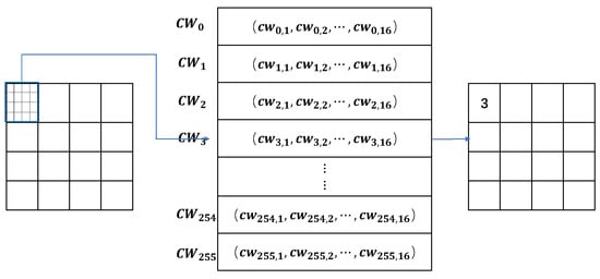
Figure 1. An example of the VQ-based image encoding ($L=256$).

2.2. Lossless Data Hiding Based on VQ Codebook Rearrangement

There are two classes of VQ-based lossless data hiding methods. The first class is to embed data in original index tables. In such schemes, a stego image can be decoded from a marked index table directly according to a standard codebook. The disadvantage of the first class’s method is that the embedding capacity is low because the redundancies of the original image are eliminated after VQ encoding. The second class is data embedding based on the rearranged codebook. It applies a codebook rearrangement technique to transfer the redundancies from a natural image to its index table and then compresses the index table to vacate the room for data embedding.

In [6], Chang et al. proposed the first VQ-based data hiding utilizing codebook rearrangement. Chang et al. [6] rearranged the codewords of a standard codebook by sorting the intensity of the codewords (SIC). The index table of a cover image, generated according to the rearranged codebook, retains a certain amount of redundancy from the original image. It generated the predicted value of an index from its neighboring indices: the one to the left, above, on the main diagonal, or on the secondary diagonal. The prediction process was carried out in raster order, and predefined indicators were used to label different cases of prediction errors. The index table generated according to the rearranged codebook was based on the SIC technique. It did not fully exploit the redundancies of the indices because it did not consider adjacent relationships in the cover image. To address this issue, Hong et al. [20] presented a different codebook rearrangement technique, called adaptive index rearrangement (AIR), which considered the adjacent relationships of indices. In the process of codebook rearrangement using the AIR technique, an occurrence frequency matrix was first constructed for a given index table. An element in the matrix denoted the occurrence frequency of two corresponding indices appearing in adjacent positions. Then, the new indices of the codewords were determined through step-by-step iteration based on the occurrence frequency matrix. In [20], the index table of a cover image, generated according to the rearranged codebook using AIR, improved the spatial correlations of indices and enhanced the efficiency of prediction error coding. In [21], Li et al. proposed a two-stage joint data embedding method. They first performed steganographic embedding on the standard index table and then calculated the difference index table based on the stego standard index table. In the second stage, data hiding was performed on the difference index table. In fact, existing methods can enhance the embedding capacity by using a steganographic embedding process similar to their first-stage embedding. Therefore, the focus of this method is to evaluate the performance of data hiding on the difference index table. Zhang et al. [31] introduced the Tabu search algorithm to find the optimal rearranged indices based on the occurrence frequency matrix. Compared to AIR, the Tabu search algorithm can slightly reduce the complexity of the index table. However, it can be seen that the key to reducing the pure compression rate of an image’s VQ stream lies in the index prediction method and the prediction difference coding method. In this paper, we present an adaptive indicator assignment method according to the vacancy capacities of prediction difference types. It improves the pure compression rate of data hiding based on VQ index table compression.

3. Proposed Scheme

In this section, a lossless data hiding scheme for VQ compressed images using adaptive prediction difference encoding is proposed. We first provide an overview of the proposed scheme. Afterward, we present the detailed procedures of data embedding, data extraction, and cover image recovery. Lastly, an example is illustrated for easier understanding of the proposed scheme.

3.1. Overview

The flowchart of the proposed lossless data hiding scheme in VQ index tables is outlined in Figure 2. We first conduct a rearrangement of the codewords in the codebook based on an adjusted AIR (adAIR) technique. According to the rearranged codebook, the original image is compressed into a VQ index table. Due to redundancy characteristics in the index table, we apply the improved MED (iMED) method to predict the index values and calculate the corresponding prediction differences between the original indices and the predicted indices. Based on the vacancy capacity of each prediction difference type, we present a prediction difference coding method to encode the prediction differences, thereby vacating embedding room for data hiding. The secret data are first encrypted and then embedded into the vacated room in the index table to generate the marked VQ index table. At the receiving end, the receiver can extract data based on the coding rules of the prediction differences and decode the prediction differences. Finally, we losslessly recover the VQ index table and then decompress it to reconstruct the cover image.

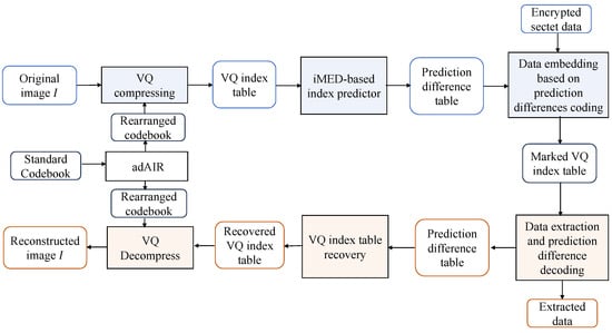
Figure 2. Flowchart of the proposed scheme.

3.2. Codebook Rearrangement

The original standard codebook is denoted by $B=\left\{{CW}_1,{CW}_2,\cdots ,W_L\right\},$ where ${CW}_i=\left({cw}_{i,1},c{w}_{i,2},\cdots ,{cw}_{i,a\times b}\right)$ for $1\le i\le L$. $L$ is the size of the codebook and is typically a power of 2. Here, we set $L$ to be $2^t$, where $t$ is a positive integer. According to the codebook, the original image $I$ with a size of $W\times H$ is compressed into an index table ${IT}_o$ using the VQ compression algorithm. Let ${IT}_o(i,j)$ denote the value in the index table ${IT}_o$ at the i-th row and j-th column, where $1\le i\le W/a,1\le j\le H/b$, and its range is $[0,2^t-1]$. It is the index value of the codeword corresponding to the image block located in the i-th row and j-th column. We use an adjusted AIR algorithm to rearrange the codebook. The details of the adjusted AIR are descripted as follows.

Step 1. Calculate the adjacency matrix $G$ with a size of $L\times L$, where the element $G(i,j)$ denotes the occurrence frequence of adjacency between the index $i$ and index $j$ in the index table ${IT}_o$. The adjacent directions include the horizontal, vertical, and downward diagonal.

Step 2. Construct a new index list $SL$ to record the new order of the codewords. The original index list of the codebook is denoted as $OL$, which is represented as $OL=\{\mathrm{0,1},\cdots ,L-1\}$. Let us assume that $G(i_1,i_2)$ is the maximum value of $G$. Then, $SL$ is initialed as $SL=\{i_1,i_2\}$ and $i_1$ and $i_2$ are deleted from $OL$. That is, $OL$ is updated as $OL=OL/\{i_1,i_2\}$.

Step 3. Perform iterative loops until $OL$ is empty. For each iteration, use Equation (3) to search for an index $i_L^{\ast }$ from $OL$ that has the maximal occurrence of adjacency to the indices of the left two-thirds of $OL$, and the corresponding maximum value is represented as ${\alpha }_L$. Meanwhile, use Equation (4) to search for an index $i_R^{\ast }$ from $OL$ that has the maximal occurrence of adjacency to the indices of the right two-thirds of $OL$, and the corresponding maximum value is represented as ${\alpha }_R$. If ${\alpha }_L\le {\alpha }_R$, then $i_R^{\ast }$ is pushed into the right of $SL$ and $OL$ is updated by deleting $i_R^{\ast }$, that is, $OL=OL/\left\{i_R^{\ast }\right\}$; otherwise, $i_L^{\ast }$ is pushed into the left of $SL$ and $OL$ should be updated as $OL=OL/\left\{i_L^{\ast }\right\}$.

$$i_L^{\ast }=\mathit{arg}\underset{i\in \mathit{OL}}{\mathit{max}}{\sum }_{j=1}^{⌊2\left|SL\right|/3⌋}G(i,SL(j\left)\right).$$

(3)

$$i_R^{\ast }=\mathit{arg}\underset{i\in \mathit{OL}}{\mathit{max}}{\sum }_{j=⌊\left|SL\right|/3⌋}^{\left|SL\right|}G(i,SL(j\left)\right).$$

(4)

Here, we search for two indices that have the maximum occurrence of adjacency within the left or right two-thirds of the list $SL$. The goal is to select an index with a high occurrence of adjacencies to $SL$ while determining the side to which the selected index should be added. Under this asymmetric computation, we ensure that the selected index maintains a high correlation with the side it is added to, while also maintaining a high overall correlation.

The final new index list $SL$ is represented as $SL=\{\tau \left(0\right),\tau \left(1\right),\cdots ,\tau \left(L-1\right)\}$, where $\tau$ is a one-to-one mapping from $\{\mathrm{0,1},\cdots ,L-1\}$ to $\{\mathrm{0,1},\cdots ,L-1\}$. Therefore, the rearranged codebook is denoted by $B_s=\left\{{CW}_{\tau \left(0\right)},{CW}_{\tau \left(1\right)},\cdots ,C{W}_{\tau \left(L-1\right)}\right\}$. According to the rearranged codebook $B_s$, the original image $I$ is compressed into a new index table ${IT}_s$ using the VQ compression algorithm.

3.3. Prediction Difference Coding and Data Embedding

In the original image, the adjacent image blocks exhibit a strong correlation, resulting in high correlation between their corresponding VQ indices. Due to the rearranged the codebook, similar code words are eventually brought together. Therefore, the VQ index table obtained after VQ compression also exhibits high redundancy, similar to that of the original image. Based on the redundancy of the VQ index table, we apply the improved MED [30] as the predictor to predict the indices and calculate the difference between the real indices and the predicted values. Furthermore, we present a prediction difference coding method to encode the prediction differences, thereby vacating the embedding room in the index table for data hiding.

3.3.1. Prediction Difference Calculation

For the VQ index table ${IT}_s$ of the original image $I$, we calculate the predicted values of the indices in ${IT}_s$ with a raster order and then compute the corresponding prediction differences to obtain a prediction difference table $D$. ${IT}_s\left(i,j\right)$ denotes the index located in the i-th row and j-th column, where $1\le i\le w/a,1\le j\le h/b$, and the predicted value $\widehat{{IT}_s}\left(i,j\right)$ of the index ${IT}_s\left(i,j\right)$ is calculated as follows:

$$\widehat{{IT}_s}\left(i,j\right)=\left\{\begin{array}{l}{IT}_s\left(i,j-1\right),ifi=1,j>1\\ {IT}_s\left(i-1,j\right),ifj=1,i>1\\ P\left({IT}_s\left(i,j\right)\right),ifi>1,j>1\end{array}\right.,$$

(5)

and the function $P$ is defined as follows:

$$P\left({IT}_s\left(i,j\right)\right)=\left\{\begin{array}{ll}\min \{x,y\},& ifz\ge \max \{x,y\}\\ \max \left\{x,y\right\},& ifz\le \min \left\{x,y\right\}\\ x+y-z,& \mathrm{otherwise}\end{array}\right.,$$

(6)

where $x={IT}_s\left(i,j-1\right)$, $y={IT}_s\left(i-1,j\right)$, and $z={IT}_s\left(i-1,j-1\right)$. Then, calculate the prediction difference $D(i,j)$ between the real index value and the predicted value using the XOR operation as follows:

$$D(i,j)=\widehat{{IT}_s}\left(i,j\right)⨁{IT}_s\left(i,j\right)$$

(7)

3.3.2. Prediction Difference Coding

Based on the prediction difference, we can determine the number of consecutive identical high significance bits (HSBs) between an original index and its predicted value. The number of consecutive identical HSBs between $IT\left(i,j\right)$ and $\widehat{IT}\left(i,j\right)$ is denoted by $N(i,j)$ and can be calculated as follows:

$$N(i,j)=t-⌈{log}_2^{D\left(i,j\right)+1}⌉.$$

(8)

The value range of $N(i,j)$ is from 0 to $t$. Therefore, $N(i,j)$ can take on $(t+1)$ possible values. To reduce the cost of storing the prediction differences, we apply adaptive binary tree encoding to label the different possible values of $N(i,j)$.

Let us assume that the total number of types used to label possible values is $k$. Figure 3 shows two binary coding trees, which are designed according to whether the number of leaf nodes k is odd or even. A path from the root node to each leaf node represents a unique code that will be used to label a type of possible value. Thus, if k is an odd number, then k types of the codes are {00, 01, 100, 101,$\cdots ,\underset{c}{\underbrace{11\cdots 1}}00$, $\underset{c}{\underbrace{11\cdots 1}}01$, $\underset{c}{\underbrace{11\cdots 1}}10, \underset{c}{\underbrace{11\cdots 1}}110$, $\underset{c}{\underbrace{11\cdots 1}}111$}, where $c=(k-1)/2-2$; if k is an even number, then k types of codes are {00, 01, 100, 101,$\cdots ,\underset{c}{\underbrace{11\cdots 1}}00$, $\underset{c}{\underbrace{11\cdots 1}}01$, $\underset{c}{\underbrace{11\cdots 1}}10, \underset{c}{\underbrace{11\cdots 1}}11$,}, where $c=k/2-2$. The difference between the two cases is at the bottom portions of the coding trees.

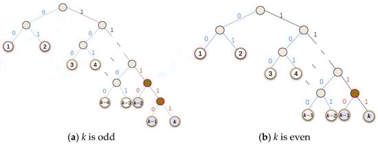
Figure 3. Binary coding tree with k types.

In our scheme, we classify the prediction differences into t types, as shown in Table 1. Type 1 denotes that the prediction difference is 0, meaning that the number of identical HSBs between the original index and its predicted values is $t$. Type 2 denotes that the number of identical HSBs is $(t-1).$ Type $i$ denotes that the prediction difference is within $[2^{i-2},2^{i-1})$, meaning that the number of identical HSBs is $t-i+1$, where $3\le i\le t-1$. Finally, for the prediction differences greater than $2^{t-2}-1$, we classify them into Type $t$, where the number of identical HSBs is 0 or 1. To assign the binary tree codes to label the t types of prediction differences, we first define a vacancy capacity for the $i$-th type as follows:

$$TC\left(i\right)=h\left(i\right)\ast (t-i+1),$$

(9)

where $h\left(i\right)$ represents the occurrence frequency of type $i$ in the entire prediction difference table $D$. Then, we sort the vacancy capacity sequence $TC$ in a descend ordering to obtain a sorted sequence $(TC\left(\sigma \left(1\right)\right),TC\left(\sigma \left(2\right)\right),\cdots ,TC\left(\sigma \left(t\right)\right))$, where $\sigma$ is a one-to-one mapping from $\{\mathrm{1,2},\cdots ,t\}$ to $\{\mathrm{1,2},\cdots ,t\}$, and $TC\left(\sigma \left(i\right)\right)>TC\left(\sigma \left(j\right)\right)$ when $i<j$. The designed codes are assigned to the t types of prediction differences as indicators according to the order $(\sigma \left(1\right),\sigma \left(2\right),\cdots ,\sigma \left(t\right)$), which is shown in Table 2.

Table 1. Classification of the prediction differences.

Type	1	2	$3$	4	$\cdots$	t − 2	t − 1	t
Prediction difference	0	1	$\left[\mathrm{2,4}\right)$	$\left[\mathrm{4,7}\right)$	$\cdots$	${[2}^{t-4},2^{t-3})$	${[2}^{t-3},2^{t-2})$	$\ge 2^{t-2}-1$
Number of identical HSBs	$t$	$t-1$	$t-2$	$t-3$	$\cdots$	3	2	$\le 1$
Frequency	$h\left(1\right)$	$h\left(2\right)$	$h\left(3\right)$	$h\left(4\right)$	$\cdots$	$h\left(t-2\right)$	$h\left(t-1\right)$	$h\left(t\right)$

Table 2. The coding rules for prediction difference types.

Type	$\mathit{\sigma }\left(1\right)$	$\mathit{\sigma }\left(2\right)$	$\mathit{\sigma }\left(3\right)$	$\mathit{\sigma }\left(4\right)$	$\cdots$	$\mathit{\sigma }\left(\mathit{t}-3\right)$	$\mathit{\sigma }\left(\mathit{t}-2\right)$	$\mathit{\sigma }\left(\mathit{t}-1\right)$	$\mathit{\sigma }\left(\mathit{t}\right)$
Indicator (t is even)	00	01	100	101	$\cdots$	$\underset{t/2-2}{\underbrace{11\cdots 1}}00$	$\underset{t/2-2}{\underbrace{11\cdots 1}}01$	$\underset{t/2-2}{\underbrace{11\cdots 1}10}$	$\underset{t/2-2}{\underbrace{11\cdots 1}11}$
Indicator (t is odd)	00	01	100	101	$\cdots$	$\underset{(t-1)/2-2}{\underbrace{11\cdots 1}01}$	$\underset{(t-1)/2-2}{\underbrace{11\cdots 1}11}$	$\underset{(t-1)/2-2}{\underbrace{11\cdots 1}110}$	$\underset{(t-1)/2-2}{\underbrace{11\cdots 1}111}$

3.3.3. Data Embedding

In the index table ${IT}_s$, the index value is represented by a $t$-bit binary. According to the prediction method, we can recover an index using the prediction difference. Therefore, we only need to record the prediction differences for each index except for the first one. We first calculate vacancy capacities for each prediction difference types of the index table, and then determine the types order $(\sigma \left(1\right),\sigma \left(2\right),\cdots ,\sigma \left(t\right)$). We can reduce the storage cost of an index table and vacate the embedding room for data hiding using the adaptive prediction difference coding. In the data embedding process, we use indicators to label the types of the prediction differences and embed secret data in the vacated room.

For the index value ${IT}_s\left(i,j\right)$ except for the first one, the data embedding procedure is presented as follows:

Step 1. Calculate the predicted value $\widehat{{IT}_s}\left(i,j\right)$ of the index value ${IT}_s\left(i,j\right)$ by Equation (5).

Step 2. Calculate the prediction difference $D\left(i,j\right)$ by Equation (7) and then determine $N\left(i,j\right)$ by Equation (8), which is the number of consecutive identical HSBs between $IT\left(i,j\right)$ and $\widehat{I{T}_s}\left(i,j\right)$.

Step 3. Convert the prediction difference $D\left(i,j\right)$ to the corresponding indicator according to the coding rules in Table 2, denoted as $HC\left(i,j\right)$, with its length denoted as $LC\left(i,j\right)$.

Step 4. Determine the number of low significant bits (LSBs) of ${IT}_s\left(i,j\right)$ that must be retained after coding, denoted as $LR\left(i,j\right)$. Because we can be certain that the ($N\left(i,j\right)$+1)-th HSB of ${IT}_s\left(i,j\right)$ differs from $\widehat{{IT}_s}\left(i,j\right)$, there is no need to record the $(N\left(i,j\right)$+1)-th HSB of ${IT}_s\left(i,j\right)$. Therefore, $LR\left(i,j\right)$ can be calculated as follows:

$$LR\left(i,j\right)=\left\{\begin{array}{ll}0,& ifN\left(i,j\right)=t\\ t-N\left(i,j\right)-1,& if2\le N\left(i,j\right)<t.\\ t,& ifN\left(i,j\right)\le 1\end{array}\right.$$

(10)

Retain the $LR\left(i,j\right)$ LSBs of ${IT}_s\left(i,j\right)$, denoted as $RLSB\left(i,j\right)$.

Step 5. Calculate the number of vacated bits after prediction difference coding, denoted as $VB\left(i,j\right)$. After coding, the prediction difference is converted into two parts: an indicator and the retained LSBs. Therefore, $VB\left(i,j\right)$ can be calculated as follows:

$$VB\left(i,j\right)=t-LR\left(i,j\right)-LC\left(i,j\right).$$

(11)

If $VB\left(i,j\right)$ is greater than 0, it means that we have $VB\left(i,j\right)$ bits of room available for embedding secret data. If $VB\left(i,j\right)$ is less than 0, we record the $\left|VB\left(i,j\right)\right|$ LSBs of $IT\left(i,j\right)$ in the auxiliary information sequence for index recovery during the recovery process.

Repeat step 1 to step 5 until all the indices are processed. The determined indicators of type 1 to type t are concatenated into an indicator sequence, denoted as $IS$. We use $IS$ to substitute the first $\left|\left|IS\right|\right|$ bits of the prediction differences and the original prediction difference bits are recorded in the auxiliary information sequence, where $\left|\left|IS\right|\right|$ is the length of $IS$. It is $(t^2+6t-8)$/4 when t is even and $(t^2+6t-7)$/4 when t is odd. Concatenate the auxiliary information sequence with the secret data. All the data are encrypted with a data-hiding key. Then, generate the marked index $\dot{{IT}_s}(i,j)$ after embedding $IS$ into ${IT}_s$. If $VB\left(i,j\right)>0$, $VB\left(i,j\right)$ bits of encrypted secret data are embedded into ${IT}_s\left(i,j\right)$, denoted as $s(i,j)$. Concatenate the indicator $HC\left(i,j\right)$, the retained LSBs $RLSB\left(i,j\right)$, and the encrypted data $s(i,j)$ to generate the t-bit of marked index value ${\dot{IT}}_S(i,j)$, that is

$${\dot{IT}}_S(i,j)=HC\left(i,j\right)\left|\right|RLSB\left(i,j\right)\left|\right|s\left(i,j\right).$$

(12)

If $VB\left(i,j\right)=0$, then the t-bit of marked index value $\dot{{IT}_s}(i,j)$ is generated as follows:

$$\dot{IT}(i,j)=HC\left(i,j\right)\left|\right|RLSB\left(i,j\right).$$

(13)

If $VB\left(i,j\right)<0$, the ($LR\left(i,j\right)-\left|VB\left(i,j\right)\right|$)HSBs of $RLSB\left(i,j\right)$, denoted as $RLSB\_H\left(i,j\right)$, are concatenated with the indicator $HC\left(i,j\right)$ to generate the marked index value $\dot{IT}(i,j)$, that is

$${\dot{IT}}_S\left(i,j\right)=HC\left(i,j\right)\left|\right|RLSB\_H\left(i,j\right).$$

(14)

And, the rest $\left|VB\left(i,j\right)\right|$ LSBs of $RLSB\left(i,j\right)$ are recorded in the auxiliary information sequence.

Once all the encrypted secret data are embedded into the index table, the marked index table ${\dot{IT}}_S$ is obtained. Then, the ${\dot{IT}}_S$ and the rearranged codebook $B_s$ consist of the marked VQ compression stream that is then transmitted to the receiver or restored.

3.4. Data Extraction and Cover Image Recovery

After receiving the marked VQ compressed stream, the receiver can obtain the marked index table ${\dot{IT}}_S$ and the rearranged codebook $B_s$. We can extract the secret data and recover the original VQ index table with shared data hiding key.

According to the marked index table and the codebook, the length of the code book, that is, the value of t, can be obtained. The length of the indicators sequence $\left|\left|IS\right|\right|$ can be calculated according to $t$, and then the indicators sequence $IS$ can be extracted from the $\left|\left|IS\right|\right|$ bits following ${\dot{IT}}_S\left(\mathrm{1,1}\right)$. The prediction difference coding rule table as shown in Table 2 can be constructed afterward. The data extraction and index recovery procedure in the marked index ${\dot{IT}}_S\left(i,j\right)$ after $IS$ are described as follows:

Step 1. Convert ${\dot{IT}}_S\left(i,j\right)$ into a $t$-bit binary. According to the coding tree, separate the indicator $HC\left(i,j\right)$ from the $t$-bit binary starting from the most significant bit. The length of $HC\left(i,j\right)$ is represented as $LC\left(i,j\right)$.

Step 2. According to the prediction difference coding rule table, obtain the number of consecutive identical HSBs $N\left(i,j\right)$ based on the $HC\left(i,j\right)$.

Step 3. Calculate $LR\left(i,j\right)$, the length of the retained LSBs of ${IT}_s\left(i,j\right)$, using Equation (10). Then, calculate $VB\left(i,j\right)$, the number of vacated bits after prediction difference coding, using Equation (11).

Step 4. If $VB\left(i,j\right)>0$, we extract $VB\left(i,j\right)$ bits of message from the $VB\left(i,j\right)$ LSBs of ${\dot{IT}}_S\left(i,j\right)$, denoted as $s\left(i,j\right)$. If $VB\left(i,j\right)\le 0$, there is no secret bit embedded into ${\dot{IT}}_S\left(i,j\right)$.

When all the embedded data are extracted, we decrypted it with a data hiding key and split it into two parts: the secret message and the auxiliary information sequence. Next, recover the first $\left|\left|IS\right|\right|$ bits prediction difference bits from the top $\left|\left|IS\right|\right|$ bits of the auxiliary information sequence. After that, delete the top $\left|\left|IS\right|\right|$ bits from the auxiliary information sequence.

We recover the index table ${IT}_s$ in a raster scan order started from ${IT}_s\left(\mathrm{1,2}\right)$. To recover the index ${IT}_s\left(i,j\right)$, we calculate the predicted index $\widehat{{IT}_s}\left(i,j\right)$ using the Equation (5), and then follow one of the three cases below:

Case 1: If $N\left(i,j\right)=t$, then ${IT}_s\left(i,j\right)$=$\widehat{{IT}_s}\left(i,j\right)$.

Case 2: If $2\le N\left(i,j\right)<t$, then set the first $N\left(i,j\right)$ HSBs of ${IT}_s\left(i,j\right)$ to be the same as $\widehat{{IT}_s}\left(i,j\right)$ and set the $(N\left(i,j\right)+1$)-th HSB of ${IT}_s\left(i,j\right)$ to be different from $\widehat{{IT}_s}\left(i,j\right)$. Next, if $VB\left(i,j\right)\ge 0$, then the $(t-N\left(i,j\right)-1$) LSBs of ${IT}_s\left(i,j\right)$ are set to $(t-N\left(i,j\right)-1$) bits following $HC\left(i,j\right)$ in ${\dot{IT}}_S\left(i,j\right)$; if $VB\left(i,j\right)<0$, then the $\left|VB\left(i,j\right)\right|$ LSBs of ${IT}_s\left(i,j\right)$ are set to be the top $\left|VB\left(i,j\right)\right|$ bits of the auxiliary information sequence and the middle $\left[t-N\left(i,j\right)-1-VB\left(i,j\right)\right]$ bits of ${IT}_s\left(i,j\right)$ are set to be the retained $(t-LC\left(i,j\right)$) bits of ${\dot{IT}}_S\left(i,j\right)$.

Case 3: If $N\left(i,j\right)<2$, then set the $(t-LC\left(i,j\right)$) HSBs of ${IT}_s\left(i,j\right)$ to be the remaining $(t-LC\left(i,j\right)$) bits of ${\dot{IT}}_S\left(i,j\right)$ after indicator $HC\left(i,j\right)$ and set the $LC\left(i,j\right)$ LSBs of ${IT}_s\left(i,j\right)$ to be the top $LC\left(i,j\right)$ bits of the auxiliary information sequence.

In two later cases, we delete the corresponding top bits in the auxiliary information sequence before moving on to recover the next index.

3.5. Example Illustration

In this subsection, we present an example to illustrate the process of data embedding, data extraction, and index recovery. Let us assume that the length of the codebook is 256, that is $t=8$. The prediction differences are classified into 8 types according to Table 1. Based on the coding tree with $k=8$ and the vacancy capacities of prediction different types, we can generate the coding rules for prediction differences. We assume that $(\sigma \left(1\right),\sigma \left(2\right),\cdots ,\sigma \left(8\right)$) is (1, 2, 3, 4, 5, 6, 7, and 8), and the corresponding coding rules are as shown in Table 3. We use the set of indicators {00, 01, 100, 101$,1100$, $1101$, $1110$, and $1111$} to label Type 1 through Type 8. For Type 8, we use ‘1111’ to indicate the case where the number of consecutive identical HSBs is either 0 or 1. Here, we also state the corresponding numbers of retained LSBs and the vacated bits after prediction difference encoding. We illustrate the secret data embedding only. The indicator sequence and the auxiliary information sequence are excluded.

Table 3. Coding rules of prediction differences with t = 8.

Type ID	Identical HSBs	Indicator	Retained LSBs	Vacated Room (bits)
1	8	00	0	6
2	7	01	0	6
3	6	100	1	4
4	5	101	2	3
5	4	1100	3	1
6	3	1101	4	0
7	2	1110	5	−1
8	$\le 1$	1111	8	−4

Assuming the index table ${IT}_s$ is (21, 27, 27, 30; 18, 21, 21, 31; 18, 21, 31, 30; 20, 21, 29, 29) the procedure of data embedding is shown in Figure 4. The predicted index table $\widehat{{IT}_s}$ is (21, 21, 27, 27; 21, 24, 21, 30; 18, 21, 31, 31; 18, 20, 31, 31), where the first index remains unchanged. Calculate the prediction difference table $D$ by Equation (7), and then calculate the numbers of the consecutive identical HSBs between the original index values and the predicted index by Equation (8), where the results are shown in N. Based on the numbers of identical HSBs, we determine the corresponding indicator, the number of retained LSBs, and the vacated bits after prediction difference encoding, which are shown in $HC$, $LR$, and $VB$, respectively. Because each $VB\left(i,j\right)>0$, where $1\le i,j\le 4$ and $(i,j)\ne \left(\mathrm{1,1}\right)$, the marked index ${\dot{IT}}_S\left(i,j\right)$ consists of $HC(i,j)$, $LR(i,j)$-LSBs of ${IT}_s(i,j)$, and $VB(i,j)$ bits of encrypted secret messages. The final marked index value table is ${\dot{IT}}_S$.

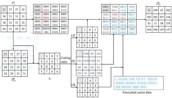
Figure 4. Example illustration of data embedding (t = 8).

The illustration of the data extraction and the index recovery is shown in Figure 5. The marked indices are converted into 8-bit binaries. Assume that the indicator sequence has been extracted. We can obtain the indicator of each index and then determine the number of retained LSBs in each index, which are shown in $HC$ and $LR$, respectively. Based on the HC and $LR$, we can calculate the number of secret data bits embedded in each marked index as shown in $VB$. According to $VB$, we extract the embedded message from the corresponding LSBs of marked indices. After the data extraction, we can recover the original indices in a raster scan ordering. Let us assume that the indices before ${IT}_s\left(\mathrm{2,2}\right)$ has been recovered. To recover ${IT}_s\left(\mathrm{2,2}\right)$, we first calculate the predicted index $\widehat{{IT}_s}\left(\mathrm{2,2}\right)$ of ${IT}_s\left(\mathrm{2,2}\right)$, which is 24. Convert ${\dot{IT}}_S\left(\mathrm{2,2}\right)$ and ${IT}_s\left(\mathrm{2,2}\right)$ into 8-bit binaries, respectively. According to the indicator sequence, we know the indicator $HC\left(\mathrm{2,2}\right)$ = ${\left(110\right)}_2$. Then, based on the coding rules, we obtain $N\left(\mathrm{2,2}\right)$ = 4 and $LR\left(\mathrm{2,2}\right)$ = 3. Because $N\left(\mathrm{2,2}\right)$ = 4, the 4 HSBs of ${IT}_s\left(\mathrm{2,2}\right)$ are the same as the bits of $\widehat{{IT}_s}\left(\mathrm{2,2}\right)$, and the 5th HSB differs from the 5-th HSB of $\widehat{{IT}_s}\left(\mathrm{2,2}\right)$. Since $LR\left(\mathrm{2,2}\right)$ = 3, we can determine that the 3 LSBs of ${IT}_s\left(\mathrm{2,2}\right)$ are the 3 bits following $HC\left(\mathrm{2,2}\right)$ in ${\dot{IT}}_S\left(\mathrm{2,2}\right)$. Therefore, ${IT}_s\left(\mathrm{2,2}\right)={\left(00010101\right)}_2$ = 21. Next, we can move on to recover the next index until we reach ${IT}_s\left(\mathrm{4,4}\right)$, which is the final index.

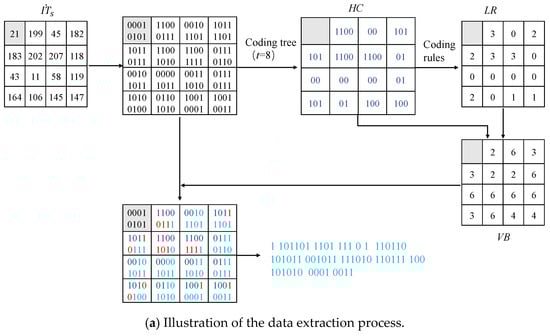
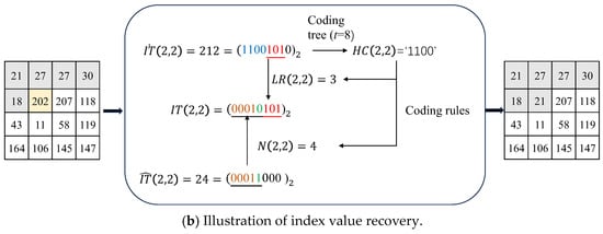
Figure 5. Illustration of data extraction and index recovery.

4. Experimental Results and Analysis

To evaluate the performance of the proposed scheme, certain experiments were conducted. We first evaluated the correlations of the indices after the codebook rearrangement. Next, we analyzed the distribution of the prediction differences to evaluate the efficiency of the predictor. Finally, we evaluated the pure compression rate and the embedding rate of proposed scheme.

4.1. Experiments Setting

In the experiments, we took eight typical standard images sized of $512\times 512$ from the USC-SIPI image database [34], including Airplane, Lena, Tiffany, Peppers, Lake, Boat, Baboon, and Goldhill, and the 24 images from Kodak dataset [35] as the test images to evaluate the performance of the proposed scheme. The size of the codebook was set to 128, 256, 512, and 1024. The block size was set to $4\times 4$. Three metrics are used to evaluate the performance of the proposed scheme, consisting of the compression rate, pure compression rate, and embedding rate. The compression rate $CR$ is defined as $\left|\right|\dot{IT}\left|\right|/(W\times H)$(bpp), where $\left|\left|\dot{IT}\right|\right|$ is the final size of the VQ index table and the $W\times H$ is the size of the original cover image. Pure compression rate $PCR$ is defined as the ratio of the sum of the size of all indicators and auxiliary information to the size of the cover image. $PCR$ is used to evaluate the efficiency of a predictor and prediction difference coding rules, and the lower $PCR$ indicates better performance. The embedding rate that denotes the average number of secret bits is embedded into each index.

4.2. Performance Analysis

In experiments, we projected all the codewords onto a base vector; we initially rearranged the codewords by sorting the projected values and then used the adAIR to obtain a codebook consisting the final rearranged codewords. Under the codebook rearrangement, we expect to enhance the correlations between adjacent indices and benefit the iMED prediction. We apply the average block complexity $C$ to evaluate the correlations between adjacent indices, which is defined as follows:

$$C={\displaystyle \frac{1}{\left(W-1\right)\ast (H-1)}}{\sum }_{i=2}^W{\sum }_{j=2}^{H}c(i,j),$$

(15)

and

$$c(i,j)={\displaystyle \frac{1}{3}}\left(\left|IT\left(i,j\right)-IT\left(i,j-1\right)\right|+\left|IT\left(i,j\right)-IT\left(i-1,j\right)\right|+\left|IT\left(i,j\right)-IT\left(i-1,j-1\right)\right|\right),$$

(16)

where $IT(i,j)$ denotes the index that locates at $(i,j)$ in the index table $IT$. $c(i,j)$ denotes the average difference in adjacent indices in the directions of left, upper, and left upper diagonal. Figure 6 shows the visualizations of the index tables using the standard codebook and the rearranged codebook on six test images, with a codebook size of 256. The first one is based on the standard codebook, and the second one is based on the rearranged codebook for each test image. We also present the corresponding average block complexity $C$ for each index table. To further demonstrate efficiency of the codebook rearrangement on reducing the block complexity, we also conduct the experiments on 24 Kodak images as shown in Figure 7. From the experiment results, we can see that the correlation of adjacent indices in index table is significantly enhanced after the codebook rearrangement, which benefits the index prediction.

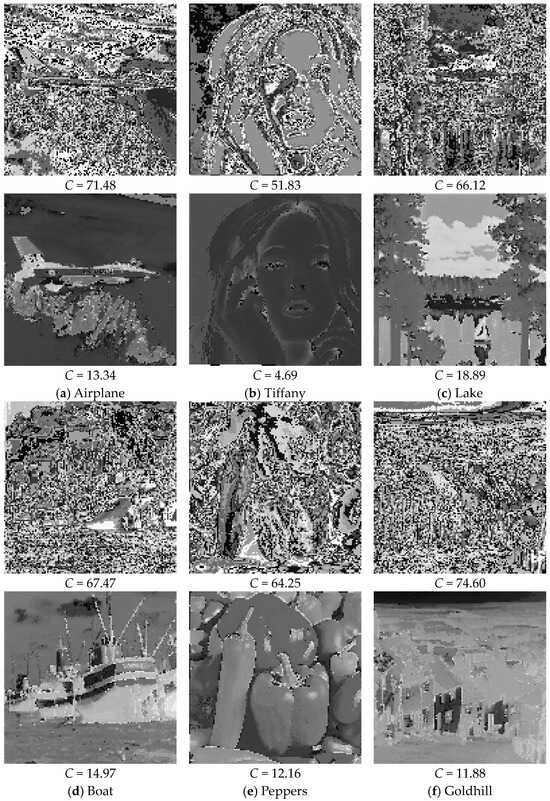
Figure 6. Visualize the index tables based on the standard codebook and the rearranged codebook of size 256 on test images.

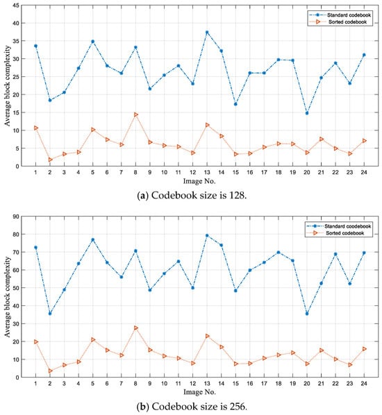
Figure 7. Average block complexity comparison on index tables using the standard codebook and the rearranged codebook on 24 Kodak images.

We assign indicators to each prediction difference type based on the vacancy capacities. Indicators encoded by the binary tree coding indicators are assigned in descending order of vacancy capacities. In Figure 8, we show the vacancy capacities of each prediction difference type on four test images using different codebook sizes. The codebook size is 256, and the vacancy capacities of prediction difference types for the test images decrease from left to right in general. The codebook’s size is 512 or 1024, the vacancy capacities vary across different test images. Type 1 has the largest vacancy capacity in most test images among all types. The size relationships of vacancy capacities of other types vary from different test images. Therefore, it is necessary to adaptively assign the indicators for different cover images based on their vacancy capacities.

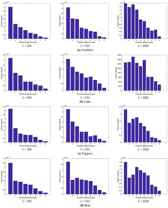
Figure 8. Vacancy capacities of each prediction type on test images.

In the proposed scheme, the maximum length of an indicator is $t/2$ when $t$ is even, and $(t+1)/2$ when $t$ is odd, where $t$ is the length of the binary representation of the index. Therefore, we can vacate the room for data embedding in index $IT(i,j)$ after prediction difference coding when $N\left(i,j\right)>⌈t/2⌉-1$, without caring which indicator is assigned to indicate its prediction difference. The proposed indicators assignment strategy can maximize the embedding capacity. According to the coding of the Equations (12)–(14) and when we keep the same compression rate for the original VQ compression stream, the embedding rate $ER$ and the pure compression rate $PCR$ of the proposed scheme can be calculated as follows:

$$ER={\displaystyle \frac{1}{W/4\times H/4}}{\sum }_{i=1}^{t}h\left(i\right)\times \left(t-L\left(i\right)-R\left(i\right)\right)],$$

(17)

and

$$PCR=[{\sum }_{i=1}^{t}h\left(i\right)\times (L\left(i\right)+R\left(i\right))]/(W\times H),$$

(18)

where $h\left(i\right)$ represents the occurrence frequency of type $i$ in the whole prediction difference table, $L\left(i\right)$ represents the length of the indicator for type $i$, and $R\left(i\right)$ represents the number of the LSBs that must be retained after encoding type $i$. We evaluate the embedding rate and the pure compression rate on four stander test images and 24 Kodak images. Figure 9 shows embedding rates on six standard test images with different codebook sizes. In the experiment, the corresponding compression rate is 0.4375, 0.5000, 0.5625, and 0.6250 when the codebook sizes are 128, 256, 512, and 1024, respectively. That is, the final length of a VQ compression stream after data embedding is the same size as the original cover index table. When the codebook size is 256 or 512, we can obtain a higher embedding rate. We can also observe that Tiffany and Airplane have higher embedding rates. This is because, after the codebook rearrangement, their index tables have lower complexity, which is validated by the experimental results in Figure 6. Figure 10 shows the pure compression rate on the six standard test images. We know the upper bound of PCRs are 0.4375, 0.5000, 0.5625, and 0.6250 when the codebook sizes are 128, 256, 512, and 1024, respectively. The results show that the proposed scheme can vacate sufficient room for data embedding. To further demonstrate the performances, we also test the proposed scheme on the 24 Kodak images, and the results are shown in Figure 11. The average embedding rates are 3.25 and 3.20, and the corresponding average pure compression rate are 0.2971 and 0.3625 when the codebook sizes are 256 and 512, respectively.

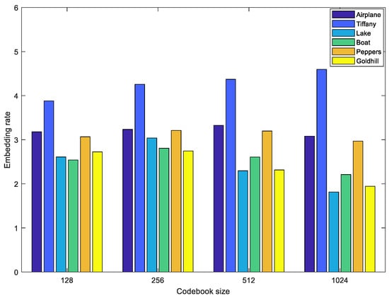
Figure 9. Embedding rates of test images under four different codebook sizes.

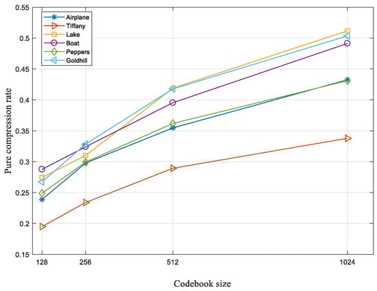
Figure 10. Pure compression rates of test images under four codebook sizes.

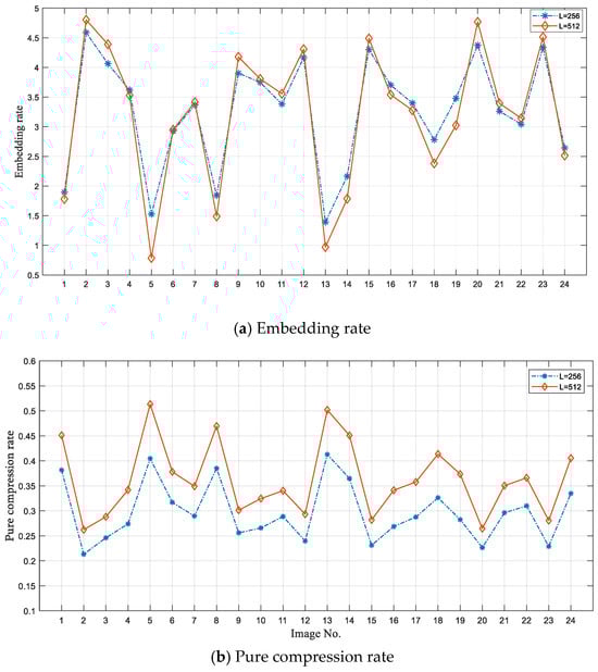
Figure 11. Performances on 24 Kodak images with codebook sizes of 256 and 512.

4.3. Comparison Experiments

In this subsection, we do performance comparisons with some related works, including Kieu and Rudder [29], Hong et al. [20], Li et al. [21], and Zhang et al. [31]. The main idea of such schemes is to rearrange the codebook and then compress the original VQ compression stream based on the redundancy of adjacent indices, thereby reducing the pure compression rate. Therefore, the lower pure compression rate indicates better performance. We show the experimental results on the pure compression rates of related works on eight standard test images in Table 4. Kieu and Rudder [29] used the SIC [6] method to resort to the codebook and used a 2- or 3-bit indicator to label the prediction errors. SIC [6] did not fully exploit the correlations of the index table. Therefore, the pure compression rates on complex images such as Baboon are not ideal. Hong et al. [20] used the AIR technique to improve the performance of the complex images. Schemes by Li et al. [21] and Zhang et al. [31] as well as the proposed scheme all continued the work based on the AIR technique. Li et al. [21] conducted two-stage data embedding in cover images. In order to ensure fairness in the comparison, we only consider data hiding in the difference index table. In the experiments, we applied the difference index table to replace our prediction difference table, while using the AIR to rearrange the codebook. The experimental results show that the proposed method has lower pure compression rates on test images compared to when conducted on difference index tables [21]. Compared to Zhang et al. [31], the proposed method achieves lower pure compression rates on test images, except for Baboon. Although Zhang et al. [31] used a weight-controlled predictor, it is difficult to match different regions with a group of weights. To further demonstrate the performance of the proposed method, we perform comparison experiments on 24 Kodak images with the method proposed by Zhang et al. [31]. In the experiments, we resized the images to $512\times 512$ as well. The experimental results are shown in Figure 12. Among the 24 test images, our method achieves a lower compression rate on 19 of them. The average pure compression rate of our method is 0.2972, while for Zhang et al. it is 0.3034. The comprehensive experimental results indicate that the proposed method is efficient and can provide a satisfactory pure compression rate on images except those with highly complex textures.

Table 4. Comparison of the pure compression rates of related works under codebook size is 256.

Image	Airplane	Lena	Tiffany	Peppers	Boat	Baboon	Goldhill
Kieu and Rudder [29]	0.307	0.349	0.283	0.335	0.342	0.492	0.389
Hong et al. [20]	0.317	0.308	0.260	0.316	0.345	0.443	0.351
Li et al. [21] (difference index)	0.316	0.321	0.248	0.316	0.343	0.448	0.335
Zhang et al. [31]	0.316	0.302	0.256	0.309	0.339	0.437	0.341
Proposed	0.298	0.281	0.234	0.299	0.324	0.440	0.328

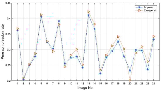
Figure 12. Comparison of the pure embedding rate over 24 Kodak images with Zhang et al. [31].

5. Conclusions

In this paper, we present a lossless data hiding scheme for VQ compressed images using an adaptive prediction difference encoding method. To enhance the correlations of adjacent indices, we used a modified AIR technique to rearrange the codebook. For the index tables based on a rearranged codebook, the improved MED predictor is used to generate the prediction differences table using the XOR operations. We define a vacancy capacity and present a coding tree to adaptively encode the prediction differences for different cover images. The prediction difference indicators, the retained bits, and the encrypted data are concatenated to generate marked VQ index tables. The experimental results on the adjacent indices show the efficiency of the codebook rearrangement. The vacancy capacity distribution analysis shows the necessity of adaptive indicator assignments. The experiments on the embedding rate and the pure compression rate show that the proposed data hiding scheme can obtain satisfying performance and outperform some related works.

References

- Shi, Y.Q.; Li, X.; Zhang, X.; Wu, H.T.; Ma, B. Reversible data hiding: Advances in the past two decades. IEEE Access 2016, 4, 3210–3237. [Google Scholar] [CrossRef]
- Tian, J. Reversible Data Embedding Using a Difference Expansion. IEEE Trans. Circuits Syst. Video Technol. 2003, 13, 890–896. [Google Scholar] [CrossRef]
- Ni, Z.; Shi, Y.Q.; Ansari, N.; Su, W. Reversible data hiding. IEEE Trans. Circuits Syst. Video Technol. 2006, 16, 354–361. [Google Scholar] [CrossRef]
- Zhang, X.; Wang, S. Efficient steganographic embedding by exploiting modification direction. IEEE Commun. Lett. 2006, 10, 781–783. [Google Scholar] [CrossRef]
- Xiong, X. An Adaptive Bit Allocation Strategy for Minimizing Embedding Distortion in Interpolated Images Used for Reversible Data Hiding. IEEE Internet Things J. 2024, 11, 20088–20098. [Google Scholar] [CrossRef]
- Chang, C.C.; Kieu, T.D.; Wu, W.C. A lossless data embedding technique by joint neighboring coding. Pattern Recognit. 2009, 42, 1597–1603. [Google Scholar] [CrossRef]
- Zhang, Y.; Luo, X.; Yang, C.; Ye, D.; Liu, F. A framework of adaptive steganography resisting JPEG compression and detection. Secur. Commun. Netw. 2016, 9, 2957–2971. [Google Scholar] [CrossRef]
- Zhang, X.; Pan, Z.; Zhou, Q.; Fan, G.; Dong, J. A reversible data hiding method based on bitmap prediction for AMBTC compressed hyperspectral images. J. Inf. Secur. Appl. 2024, 81, 103697. [Google Scholar] [CrossRef]
- Puech, W.; Chaumont, M.; Strauss, O. A reversible data hiding method for encrypted images. In Security, Forensics, Steganography, and Watermarking of Multimedia Contents X; SPIE: San Jose, CA, USA, 2008; Volume 6819, pp. 534–542. [Google Scholar] [CrossRef]
- Zhang, X. Reversible data hiding in encrypted image. IEEE Signal Process. Lett. 2011, 18, 255–258. [Google Scholar] [CrossRef]
- Fu, Z.; Chai, X.; Tang, Z.; He, X.; Gan, Z.; Cao, G. Adaptive embedding combining LBE and IBBE for high-capacity reversible data hiding in encrypted images. Signal Process. 2024, 216, 109299. [Google Scholar] [CrossRef]
- Chan, C.K.; Cheng, L.M. Hiding data in images by simple LSB substitution. Pattern Recognit. 2004, 37, 469–474. [Google Scholar] [CrossRef]
- He, W.; Cai, Z. Reversible Data Hiding Based on Dual Pairwise Prediction-Error Expansion. IEEE Trans. Image Process. 2021, 30, 5045–5055. [Google Scholar] [CrossRef] [PubMed]
- Kim, S.; Qu, X.; Sachnev, V.; Kim, H.J. Skewed Histogram Shifting for Reversible Data Hiding Using a Pair of Extreme Predictions. IEEE Trans. Circuits Syst. Video Technol. 2019, 29, 3236–3246. [Google Scholar] [CrossRef]
- Fridrich, J.; Soukal, D. Matrix embedding for large payloads. IEEE Trans. Inf. Forensics Secur. 2006, 1, 390–395. [Google Scholar] [CrossRef]
- Zhang, T.; Li, X.; Qi, W.; Guo, Z. Location-Based PVO and Adaptive Pairwise Modification for Efficient Reversible Data Hiding. IEEE Trans. Inf. Forensics Secur. 2020, 15, 2306–2319. [Google Scholar] [CrossRef]
- Wang, Y.; Xiong, G.; He, W. High-capacity reversible data hiding in encrypted images based on pixel-value-ordering and histogram shifting. Expert Syst. Appl. 2023, 211, 118600. [Google Scholar] [CrossRef]
- Wu, Y.; Hu, R.; Xiang, S. PVO-based Reversible Data Hiding Using Global Sorting and Fixed 2D Mapping Modification. IEEE Trans. Circuits Syst. Video Technol. 2023, 34, 618–631. [Google Scholar] [CrossRef]
- Qin, C.; Chang, C.C.; Chiu, Y.P. A novel joint data-hiding and compression scheme based on SMVQ and image inpainting. IEEE Trans. Image Process. 2014, 23, 969–978. [Google Scholar] [CrossRef]
- Hong, W.; Zhou, X.; Lou, D.C.; Chen, T.S.; Li, Y. Joint image coding and lossless data hiding in VQ indices using adaptive coding techniques. Inf. Sci. 2018, 463–464, 245–260. [Google Scholar] [CrossRef]
- Li, Y.; Chang, C.C.; He, M. High Capacity Reversible Data Hiding for VQ-Compressed Images Based on Difference Transformation and Mapping Technique. IEEE Access 2020, 8, 32226–32245. [Google Scholar] [CrossRef]
- Mobasseri, B.G.; Berger, R.J.; Marcinak, M.P.; Naikraikar, Y.J. Data embedding in JPEG bitstream by code mapping. IEEE Trans. Image Process. 2010, 19, 958–966. [Google Scholar] [CrossRef]
- Tang, W.; Yao, H.; Le, Y.; Qin, C. Reversible data hiding for JPEG images based on block difference model and Laplacian distribution estimation. Signal Process. 2023, 212, 109130. [Google Scholar] [CrossRef]
- Weng, S.; Zhou, Y.; Zhang, T.; Xiao, M.; Zhao, Y. Reversible Data Hiding for JPEG Images With Adaptive Multiple Two-Dimensional Histogram and Mapping Generation. IEEE Trans. Multimed. 2023, 25, 8738–8752. [Google Scholar] [CrossRef]
- Ma, K.; Zhang, W.; Zhao, X.; Yu, N.; Li, F. Reversible data hiding in encrypted images by reserving room before encryption. IEEE Trans. Inf. Forensics Secur. 2013, 8, 553–562. [Google Scholar] [CrossRef]
- Chen, S.; Chang, C.C. Reversible data hiding in encrypted images using block-based adaptive MSBs prediction. J. Inf. Secur. Appl. 2022, 69, 103297. [Google Scholar] [CrossRef]
- Yang, Y.; Chen, F.; Tai, H.M.; He, H.; Qu, L. Reversible data hiding in encrypted image based on key-controlled balanced Huffman coding. J. Inf. Secur. Appl. 2024, 84, 103833. [Google Scholar] [CrossRef]
- Wang, J.X.; Lu, Z.M. A path optional lossless data hiding scheme based on VQ joint neighboring coding. Inf. Sci. 2009, 179, 3332–3348. [Google Scholar] [CrossRef]
- Kieu, T.D.; Rudder, A. A reversible steganographic scheme for VQ indices based on joint neighboring and predictive coding. Multimed. Tools Appl. 2016, 75, 13705–13731. [Google Scholar] [CrossRef]
- Weinberger, M.J.; Seroussi, G.; Sapiro, G. From LOCO-I to the JPEG-LS standard. IEEE Int. Conf. Image Process. 1999, 4, 68–72. [Google Scholar] [CrossRef]
- Zhang, T.; Weng, S.; Wu, Z.; Lin, J.; Hong, W. Adaptive encoding based lossless data hiding method for VQ compressed images using tabu search. Inf. Sci. 2022, 602, 128–142. [Google Scholar] [CrossRef]
- Linde, Y.; Buzo, A.; Gray, R.M. An algorithm for vector quantization. IEEE Trans. Commun. 1980, 28, 84–95. [Google Scholar] [CrossRef]
- Nasrabadi, N.M.; King, R.A. Image Coding Using Vector Quantization: A Review. IEEE Trans. Commun. 1988, 36, 957–971. [Google Scholar] [CrossRef]
- Weber, A.G. The USC-SIPI Image Database: Version 5; USC Viterbi School Eng.; Signal Image Processing Institute: Los Angeles, CA, USA, 2006. [Google Scholar]
- Kodak. Kodak Lossless True Color Image Suite. Available online: http://r0k.us/graphics/kodak/index.html (accessed on 4 October 2022).
Disclaimer/Publisher’s Note: The statements, opinions and data contained in all publications are solely those of the individual author(s) and contributor(s) and not of MDPI and/or the editor(s). MDPI and/or the editor(s) disclaim responsibility for any injury to people or property resulting from any ideas, methods, instructions or products referred to in the content. |
© 2024 by the authors. Licensee MDPI, Basel, Switzerland. This article is an open access article distributed under the terms and conditions of the Creative Commons Attribution (CC BY) license (https://creativecommons.org/licenses/by/4.0/).