2.3.1. User Traffic Characteristics
Traffic prediction is based on the aggregation of each accepted tenant. Tenants may request different network slices according to their specific service requirements, without specifying the set of physical cells where their users are located. In fact, a particular vertical tenant may only require a small number of cells to provide specific services for its users. For example, the automotive industry may only need cells that cover suburban roads. Our approach involves classifying traffic requests according to relevant service requirements and geographic locations, thus enabling separate predictions for each cell and each slice. In our analysis, we initially assume that traffic requests are uniformly distributed across the entire network.
We assume the following traffic model. We assume different classes of traffic based on specific SLAs, as shown in
Table 2 [
28]. Let the traffic volumes of tenant
for traffic
be modeled as a point process,
, where
denotes the Dirac metric for sample
and
is the set of cell. We express each user’s traffic requests
as the required resource metric, and for each user
express the aggregate traffic as
.
2.3.2. Traffic Forecasting
In our model, a fundamental key assumption is that traffic requests follow a cyclical pattern, which is essential for applying time series forecasting algorithms. Based on the assumed periodicity, traffic forecasting is conducted based on an observed time window and is represented by a vector, , . Then, we fix a future time window that provides the predicted traffic for the time period , , , through a forecast function . As the observed time window extends and more information is collected, the accuracy of traffic predictions for each user’s slice in the future time window increases.
Under the above assumptions, the system exhibits periodic behavior, where
represents a season that repeats over time. Within a single season, we assume that the process
is stationary and ergodic [
29]:
where
expresses the average traffic request for the
type of traffic of the
user,
represents the number of units, and
defined as the
type of traffic request for the
user at time
.
To this end, we use the Holt–Winters (HW) forecasting method to analyze and predict future traffic requests associated with specific network slices across all selected cells. The definition of the forecasting function
is as follows:
We denote a specific predicted traffic request
by
. We use the additive version of the HW forecasting model, as the seasonal effect does not depend on the mean traffic level of the observed time window but is instead added based on values predicted through level and trend effects. Following the standard HW procedure and assuming a seasonality frequency (W) based on traffic characteristics, we can predict such requests using the level
, trend
, and seasonal
factors, as follows:
where
denotes the integer part of
and the set of optimal HW parameters
,
, and
can be obtained during a training period employing existing techniques. We focus on how prediction errors and inaccuracies affect our network slicing solutions. Inaccurate predicted traffic values may lead to incorrect embedding of network slices, which in turn may fail to adapt to the system’s capacity, resulting in degraded service quality. Therefore, the training prediction error is further defined as follows:
which can be computed during the training of the prediction algorithm. For any predicted value at time y, where a prediction interval
can be derived for which the error probability of future traffic requests is
for that particular network slice request. Given that our process
is iterative, assuming an optimal set of hardware parameters, for any predicted value at time
, we can derive the prediction interval
with a certain probability
for future traffic requests specific to our network slice. Therefore, it is considered that
where
,
denotes the one-tailed value of a standard normal distribution,
,
expresses the probability, and
is the variance of the one-step training prediction error over the observed time window, i.e.,
.
Due to the requirements imposed by traffic SLAs, we focus only on the upper bound of the prediction interval as it provides the “worst-case” of a forecasted traffic level. Following the above, best-effort traffic requests with no stringent requirements can tolerate a prediction with a longer time pace that results in imprecise values. This makes the upper bound very close to the future value regardless of the error probability ; the number of predicted values is finite. On the other hand, when considering the need to meet bit rate traffic requirements within a shorter period, the forecasting process becomes more complex and requires more predicted values . Such traffic needs to be modeled with a higher probability of prediction error probability .
According to the traffic categories defined in
Table 1, the traffic category
requires a shorter prediction range than the other traffic categories, and therefore further predictions are necessary, for which an upper bound on the prediction probability error per user for that traffic category is derived. We define the maximum gain between sliced requests and predicted traffic requests as
. Then, the prediction error probability is as follows:
As soon as the potential gain becomes very large, we cap the one-tailed value to 3.49, resulting in = 99.9%. Conversely, for the best-effort traffic ( = 4), we compute the forecasting error probability = 50%, due to its more relaxed service. For the other traffic classes , intermediate forecasting error probabilities are calculated from (6) by deriving values from the upper and the lower bound values.
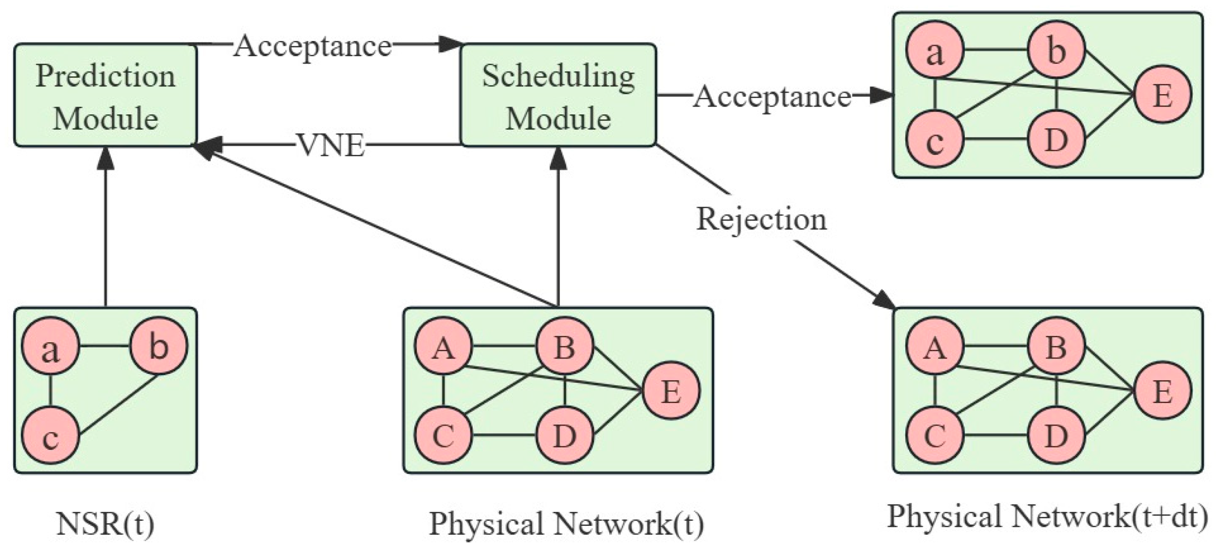
2.3.3. Scheduling Model
We define the network slicing request as , where is the amount of resources required, is the duration of the slice, denotes the tenant, and is the traffic class. In general, the user requests are denoted as and the traffic classes are predicted for a fixed time window . We assume that the physical network resources are a rectangular box that represents a limited amount of resources. where the width corresponds to and the height corresponds to the total amount of available resources . The cost of each network slice request is proportional to the amount of resources requested . The allocation of resources is an NP-hard problem.
The amount of resources required per time
based on the predicted traffic type
(with a given prediction error probability
) is denoted by the set
, and
denotes the requests of user
for category
. Five traffic categories shown in
Table 1 are considered, each characterized by a time window
that identifies the duration
over which the category should see the metric, which is shorter for highly demanding traffic categories and longer for more moderate categories. The scheduling module will give the appropriate amount of resources
to meet the traffic metric within this length.
To ensure that the scheduling module expects the network slice traffic level to be no lower than the predicted traffic boundary,
. The key goal of the scheduling module is to minimize the consumed resources, i.e., minimize the cost, while guaranteeing the SLA of the traffic within the network slice by setting a time window
that will encompass all classes of time windows
,
. The mathematical model of the scheduling module is established as follows:
where
is the total capacity of physical resources,
is the penalty generated by not meeting the SLA of the user’s network slicing service used for feedback prediction,
is a larger constant factor set to ensure the reduction in
always has the highest priority,
is to determine whether to accept the request, acceptance is 1, and refusal is 0.
The prediction error probability for the general flow category can be derived from Equation (6):
as a historical penalty function, is defined as follows:
where
is defined as the number of times the penalty is zero,
.
is defined as the length of the season in the forecasting process. The historical penalty function sets the control policy in order to control the system from SLA violations, derives a larger prediction error probability
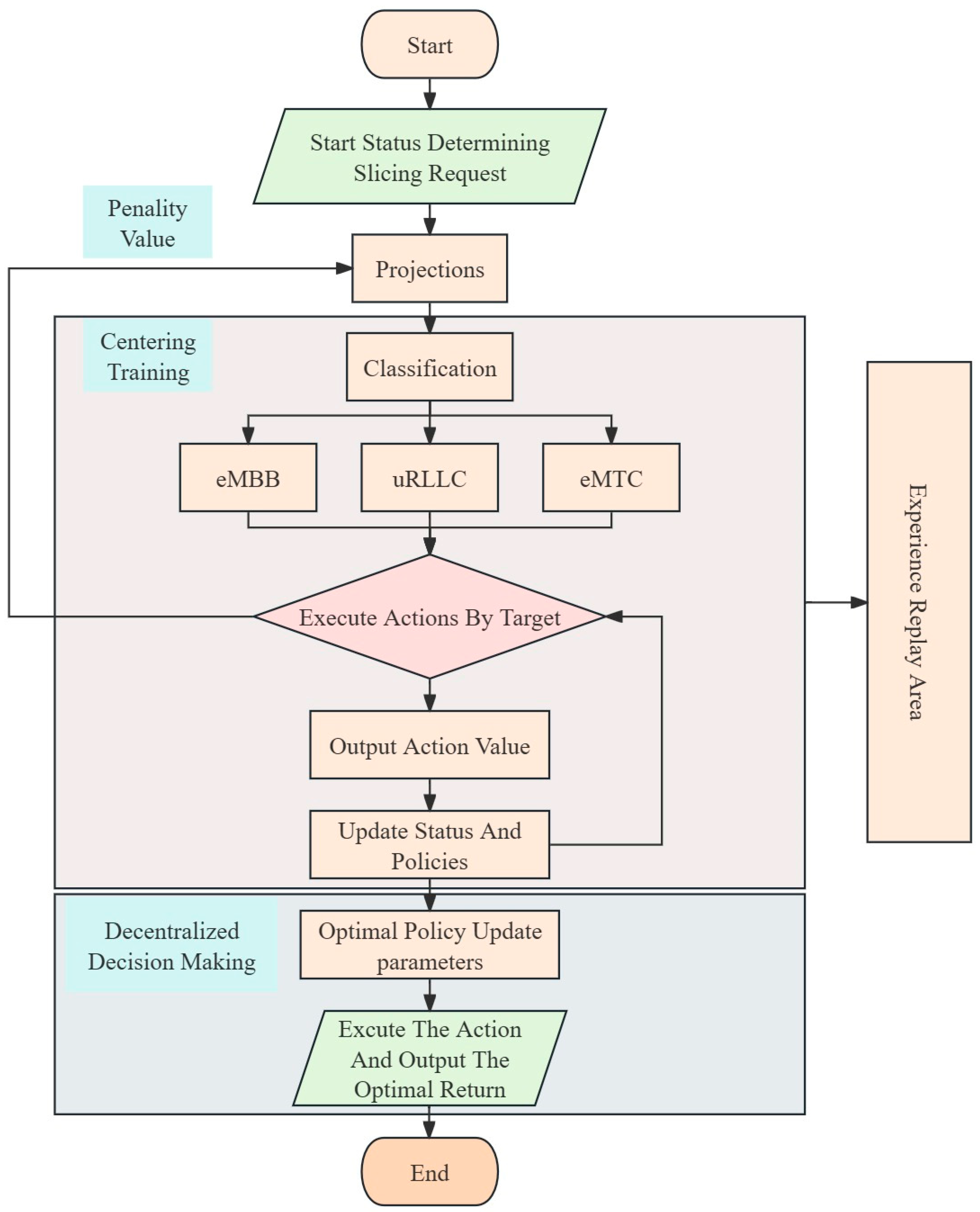
in the case of prediction failure, obtains a smaller gain, and prevents the waste of resources. The objective of setting three types of slices determines the metric
of each user traffic request in the prediction model.
eMBB: Enhanced mobile broadband is a key application scenario of 5G technology, aiming to provide wide-area coverage and hotspot connectivity. In hotspot scenarios, where user density is high, there is a need for very high traffic capacity, while the requirements for mobility are lower and user data rates are higher. This type of slice does not require strict delay constraints or abundant resources. Therefore, the deployment goal of eMBB slices should be to maximize the remaining resources on physical nodes, which can be represented as follows:
where
and
represent the sets of physical nodes and virtual nodes, respectively,
denotes the resource capacity of physical node,
denotes the resource demand of virtual node, and
represents the mapping relationship of virtual node
on physical node
.
mMTC: Massive machine-type communications (mMTC) primarily address the large-scale connectivity needs of Internet of Things (IoT) devices, characterized by a vast number of connected devices, typically transmitting low volumes of data with latency insensitivity. Due to the need to handle a large number of connections, there is a high demand for computational resources and low congestion rates. Consequently, this type of slice aims to minimize bandwidth usage on physical links. In other words, it should maximize the remaining bandwidth on physical links. Therefore, the deployment objective for mMTC slices can be expressed as follows:
where
and
represent the sets of physical link and virtual link, respectively,
represents the bandwidth of the physical link,
denotes the bandwidth of the virtual link, and
represents the number of virtual links corresponding to the physical link.
uRLLC: Ultra-reliable low-latency communication aims to provide extremely high reliability and very low communication latency to meet the needs of applications requiring high real-time performance and stability. uRLLC has strict latency requirements, and the deployment objective should be to minimize the slice’s latency. We translate latency time into hops, so minimizing latency is equivalent to minimizing the length of each physical path. Therefore, the deployment objective for uRLLC slices is as follows:
The constraints corresponding to the overall deployment objectives are as follows:
where the constraints of the above equation are expressed as follows: (a) each virtual node is guaranteed to be mapped to only one physical node; (b) each physical node is guaranteed to host only one virtual node; (c) ensuring that the bandwidth occupied by each node does not exceed the total available bandwidth.
In order to meet the demands of the virtual nodes, it is necessary to add two constraints to ensure that the resource capacity of each physical node can meet the total demand of the virtual nodes mapped to it. At the same time, we ensure that the available computing resources of the physical nodes mapping the virtual nodes are not less than the demands of the virtual nodes, which can be expressed as follows:


