Mobile Robot Navigation Based on Noisy N-Step Dueling Double Deep Q-Network and Prioritized Experience Replay

Abstract

Effective real-time autonomous navigation for mobile robots in static and dynamic environments has become a challenging and active research topic. Although the simultaneous localization and mapping (SLAM) algorithm offers a solution, it often heavily relies on complex global and local maps, resulting in significant computational demands, slower convergence rates, and prolonged training times. In response to these challenges, this paper presents a novel algorithm called PER-n₂D₃QN, which integrates prioritized experience replay, a noisy network with factorized Gaussian noise, n-step learning, and a dueling structure into a double deep Q-network. This combination enhances the efficiency of experience replay, facilitates exploration, and provides more accurate Q-value estimates, thereby significantly improving the performance of autonomous navigation for mobile robots. To further bolster the stability and robustness, meaningful improvements, such as target “soft” updates and the gradient clipping mechanism, are employed. Additionally, a novel and powerful target-oriented reshaping reward function is designed to expedite learning. The proposed model is validated through extensive experiments using the robot operating system (ROS) and Gazebo simulation environment. Furthermore, to more specifically reflect the complexity of the simulation environment, this paper presents a quantitative analysis of the simulation environment. The experimental results demonstrate that PER-n₂D₃QN exhibits heightened accuracy, accelerated convergence rates, and enhanced robustness in both static and dynamic scenarios.

1. Introduction

Mobile robots play an increasingly crucial role in various aspects of our daily lives and work, including agricultural operations, catering services, medical assistance, military actions, autonomous driving, etc. The successful execution of tasks in these applications hinges on the mobile robots’ adept navigation through static or dynamic environments, coupled with collision avoidance [1,2]. Effective navigation requires mobile robots to accurately sense and respond to their surroundings, especially in dynamic settings, where robots confront evolving terrains, dynamic obstacles, and unforeseen scenarios, necessitating the capability to explore and learn to proficiently adapt to changing environments.

Simultaneous localization and mapping (SLAM) has emerged as a solution, integrating the mobile robot’s position and environmental state data from sensors to construct precise local and global maps for autonomous navigation [3]. However, this process relies on costly sensors and manual examinations to guarantee that the produced maps satisfy the required standards for path planning and localization, which may hamper its efficiency by consuming time, resources, and computational power [4,5]. Recently, visual SLAM has been used for robot navigation, relying on a visual camera to capture environmental images and calculate the robot’s position and direction. Nevertheless, its susceptibility to external factors, such as light, humidity, temperature variations, and dust, coupled with computational demands in complex environments, raises concerns about accuracy and performance [6].

In response, deep reinforcement learning (DRL) was proposed and has gained prominence in autonomous navigation [7]. This paradigm introduces an innovative approach to decision-making from raw sensor inputs in diverse environments through the fusion of deep learning (DL) and reinforcement learning (RL). On the one hand, DRL leverages DL’s success in high-dimensional information analysis, especially in image analysis, speech recognition, and natural language processing, which has yielded a spectrum of supervised and unsupervised DL algorithms tailored for the movement of mobile robots [8]. Such algorithms have proven effective in tasks like path planning and navigation [9]. On the other hand, DRL harnesses the efficacy of RL in addressing challenges in sequential decision-making [10]. This empowers the agent to gradually learn optimal decision strategies to maximize cumulative rewards or achieve specific goals through interactions with its environment [11,12].

As an end-to-end DRL algorithm, the deep Q-Network (DQN) was introduced [13], and its success in learning policies from high-dimensional inputs was demonstrated. To enhance learning efficiency and stability, the algorithm utilizes an experience replay buffer to store and reuse previous experiences. Additionally, a secondary target network is introduced to address issues of oscillation and divergence during the learning process. Despite the DQN’s success in diverse applications and its widespread use in autonomous navigation [14,15], it has some drawbacks, notably action value overestimation derived from Q-learning updates. This overestimation arises because the action with the highest value in the Q-network is usually selected in the next state, and the same Q-network is used to select actions and calculate action values. This approach can lead to overestimation issues, as it does not consider the possibility of estimation errors. To address this issue, the double deep Q-network (DDQN) was proposed [16], utilizing two distinct Q-networks for action selection and value estimation to prevent overestimation. Meanwhile, DDQN finds applications in training mobile robots for tasks like optimal navigation and obstacle avoidance [17,18].

This research initially used the DQN algorithm to solve autonomous navigation for mobile robots. Although the accuracy can reach over 95% in open and enclosed simulation environments, with the increase in obstacles, the accuracy with the original DQN algorithm is very low. Then, the DDQN algorithm was utilized to enhance the accuracy, but the performance improvement was still minor. On the other hand, the rainbow DDQN with multiple improvement techniques has greatly improved the performance of the DDQN in Atari games [19] with high-dimensional, complex state and action spaces. However, autonomous navigation for mobile robots may have relatively low-dimensional state and action spaces, but it requires a fast response with a low computational load. The rainbow DDQN may be overly complex and inefficient for our purpose and may also increase the difficulty of implementation and parameter adjustment. More importantly, the rainbow DDQN may require more computational resources and training time, which might be challenging in resource-constrained environments or scenarios requiring rapid iteration.

In autonomous navigation problems for mobile robots, there is usually a high correlation between states. However, the traditional experience replay method in the DDQN randomly samples with equal probability, ignoring the importance of different samples, thus leading to a long training time and making it difficult to converge. Additionally, in the DDQN algorithm, the agent adopts an $ϵ$-greedy algorithm for exploration, which conducts random exploration with a probability of $ϵ$ and selects the current optimal action with a probability of 1 $-ϵ$, leading the performance to heavily rely on the size of $ϵ$. Furthermore, the $ϵ$-greedy algorithm selects the optimal action based on the current maximum Q-value at each time step, ignoring opportunities to explore other unknown actions, meaning that it may fall into a local optimal solution and fail to discover the global optimal solution. Although the DDQN can alleviate the overestimation problem to a certain extent, in mobile robot autonomous navigation problems, states typically exhibit a strong correlation. There still exists the potential for overestimation in certain actions because the Q-values of different actions may be highly similar, making it difficult to accurately estimate their differences. In this case, the network may overestimate the values of certain actions, leading to unstable learning.

To solve the aforementioned problems and propose an efficient mapless autonomous navigation algorithm for mobile robots with high accuracy in both static and dynamic environments, this paper introduces a novel variant of the DDQN named prioritized experience replay noisy n-step dueling DDQN (PER-n₂D₃QN). As implied by its name, this proposed method incorporates a key enhancement by replacing traditional experience replay with prioritized experience replay (PER), where each experience is assigned a priority based on its significance or informativeness. This prioritization mechanism allows the agent to focus on the experiences that most significantly contribute to its learning objectives, enhancing the sample efficiency [20,21]. Furthermore, a noisy network [22] with factorized Gaussian noise injected into the parameters of the online network is introduced to solve the exploration limitation in the DDQN, which can automatically adjust the randomness of action selection to find a better balance between exploration and exploitation. Additionally, an n-step temporal difference learning mechanism is adopted to alleviate the estimation error of the target Q-value, moving much closer to the real target Q-value [23], coupled with a dueling network structure to further alleviate overestimation issues and improve the stability and accuracy of learning by decomposing the Q-value into a state-value function and an advantage function, allowing the network to better learn the relationship between the state value and action advantage [24,25].

The main contributions of this paper are outlined as follows:

(1) The PER-n₂D₃QN algorithm, integrating PER, a noisy network, n-step learning, and a dueling architecture, is employed in autonomous navigation for mobile robots, significantly boosting navigation performance and accuracy.

(2) To enhance the stability and robustness of the algorithm, some enhancements are also applied to the proposed algorithm, such as a target “soft” update and a gradient clipping mechanism.

(3) A novel, effective target-oriented reshaping reward function is employed to guide the mobile robot toward the designated point while avoiding obstacles, thereby expediting convergence.

(4) In order to more specifically reflect the complexity of the simulation environment, this paper presents a detailed quantitative analysis of the simulation environment for the first time.

(5) The performance of PER-n₂D₃QN is validated through numerical simulation experiments with the ROS and Gazebo, and the results demonstrate that PER-n₂D₃QN exhibits superior performance in autonomous navigation for mobile robots compared to the DQN and DDQN, coupled with showing the whole path processed by the PER-n₂D₃QN algorithm within an episode.

The rest of this paper is structured as follows: Section 2 presents the problem statement and related research. Section 3 details the methodology of the proposed PER-n₂D₃QN. Section 4 provides implementation details for PER-n₂D₃QN. Section 5 presents the experimental setting and result analysis of the DQN, DDQN, and PER-n₂D₃QN algorithms. Finally, Section 6 concludes the paper with insights and future research directions.

2. Background

2.1. Problem Statement

The increasing deployment of mobile robots across various sectors highlights the critical need to enable them to autonomously navigate while avoiding collisions. Traditional mobile robot navigation faces challenges, including difficulties in environment perception, path planning, and real-time decision-making. To solve these problems, DRL algorithms, particularly those focused on goal-searching mapless navigation, have gained widespread use in autonomous robot navigation [26,27,28].

Among them, DDQN technology has demonstrated significant potential. However, a notable challenge remains in achieving real-time and high-accuracy mobile robot navigation in both static and dynamic environments using the original DDQN algorithms. Hence, this paper aims to address this challenge by advancing research in the field of mobile robot autonomous navigation, striving to offer more efficient, accurate, and safe solutions for mobile robot navigation tasks.

2.2. Reinforcement Learning Basics

In reinforcement learning (RL), the Markov Decision Process (MDP) is often employed to model stochastic state transitions of the environment and subsequent decision-making [29]. An MDP comprises four essential elements: S, A, R, and P. At each time step t, the agent observes the environment’s state $s_t\in S$, where S is the state space. Based on this observation, the agent selects an action $a_t$ from the action space A. After executing an action $a_t$, the agent receives a reward, $r_t\in R$, where R represents the rewards obtained by the agent from interacting with the environment. Subsequently, the state transitions to $s_{t+1}$ from $s_t$ with a certain probability $p_t\in P$. In RL, the tuple ($s_t$, $a_t$, $r_t$, $s_{t+1}$) is referred to as an experience sequence. The relationship between S, A, R, and P is depicted in Figure 1.

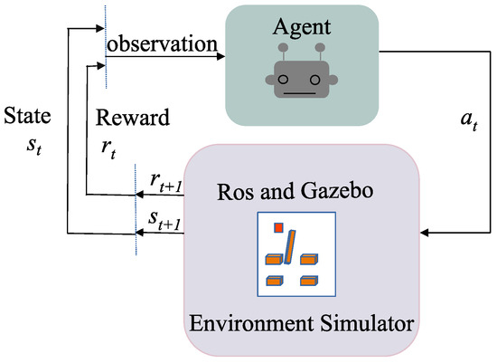
Figure 1. The structure of an MDP, where $s_t$ is the environment state at time step t, $a_t$ denotes the action taken by the agent in state $s_t$, and $r_t$ is the reward received from the environment at time step t.

Although the agent receives a reward for each step in the process of interacting with the environment, the ultimate goal is to maximize the sum of rewards, defined as the expected return in RL. By introducing the discount factor $\gamma \in \left[0,1\right]$, the expected return is defined as the discounted accumulated rewards obtained since the current time step t as follows:

$$\begin{array}{c}{G}_t=\sum _{k=0}^{\infty }{\gamma }^k{r}_{t+k},\hfill \end{array}$$

(1)

where the value of the discount factor $\gamma$ influences how much importance the agent assigns to immediate and future rewards. A higher $\gamma$ implies a more forward-looking agent, while a lower $\gamma$ indicates a more immediate-reward-focused agent. Policy $\pi$ determines the action the agent should take in different environments and is a mapping from a state to the probability of choosing each action [30]. The state-value function $V^{\pi }\left(s\right)$ under a certain policy $\pi$ can be defined as follows:

$$\begin{array}{c}{V}^{\pi }\left(s\right)=\mathbb{E}[\sum _{k=0}^{\infty }{\gamma }^k{r}_{t+k}\mid s_t=s],\hfill \end{array}$$

(2)

where $\mathbb{E}$[.] is an expectation function. Similarly, under a certain policy $\pi$, the action-value function $Q^{\pi }(s,a)$ is the expected return after executing action a starting from state s:

$$\begin{array}{c}{Q}^{\pi }(s,a)=\mathbb{E}[\sum _{k=0}^{\infty }{\gamma }^k{r}_{t+k}\mid s_t=s,a_t=a].\hfill \end{array}$$

(3)

According to Equation (2), different policies $\pi$ may correspond to different values in the state-value function. Among all policies, there is at least one policy, ${\pi }^{*}$, that maximizes the value of the state-value function in state s, and ${\pi }^{*}$ is called the optimal policy. The state-value function under the optimal policy ${\pi }^{*}$ is called the optimal state-value function $V^{*}\left(s\right)$:

$$\begin{array}{c}{V}^{*}\left(s\right)={max}_{\pi }{V}^{\pi }\left(s\right)={max}_{\pi }\mathbb{E}[r_t+\gamma G_{t+1}\mid s_t=s].\hfill \end{array}$$

(4)

Similarly, the action-value function under the optimal policy ${\pi }^{*}$ is called the optimal action-value function $Q^{*}(s,a)$ and is defined as follows:

$$\begin{array}{c}{Q}^{*}(s,a)=\mathbb{E}[r_t+\gamma \underset{a^{\prime }}{max}{Q}^{*}(s_{t+1},a^{\prime })\mid s_t=s,a_t=a].\hfill \end{array}$$

(5)

2.3. One-Step and N-Step TD Methods

For the purpose of estimating the action-value function, an off-policy temporal difference (TD) algorithm called Q-learning was proposed [14]. Q-learning uses Q-tables to store Q-values for each state–action pair and updates $Q(s_t,a_t)$ as follows:

$$\begin{array}{cc}{Q}_t(s_t,a_t)\hfill & =Q_t(s_t,a_t)+\eta [y_t-Q(s_t,a_t)],\hfill \end{array}$$

(6)

where $\eta \in [0,1]$ is the learning rate, controlling the magnitudes for updating Q-values. In Equation (6), $y_t$ is called the TD target value, which is used to approximate the discounted accumulated reward $G_t$. For a one-step TD algorithm, the time-step gap between the estimated state–action pairs is only one time step, and just one time-step reward $r_t$ is promptly utilized in each update [31]. The one-step TD target value $y_t^{\left(1\right)}$ can be expressed as follows:

$$\begin{array}{c}{y}_t^{\left(1\right)}=r_t+\gamma \underset{a^{\prime }}{max}Q(s_{t+1},a^{\prime }).\hfill \end{array}$$

(7)

In the one-step TD method, if $y_t^{\left(1\right)}$ is not equal to $G_t$, then the TD target value is slightly biased. To solve this problem and incorporate longer trajectories containing more information about future rewards, the n-step TD algorithm was proposed [23]. This approach enhances the learning efficiency of the one-step TD algorithm by bootstrapping over more time steps. N-step TD methods, such as n-step Q-learning [14] and n-step sarsa [23], consider the accumulated rewards in the next n steps and the state estimation after n time steps to update the action-value function. This allows the algorithm to exploit long-term, high-reward strategies from past experiences and further improve the efficiency of the reward signal. The n-step TD target value $y_t^{\left(n\right)}$ can be written as follows:

$$\begin{array}{c}{y}_t^{\left(n\right)}=\sum _{k=0}^{n-1}{\gamma }^k{r}_{t+k}+{\gamma }^n\underset{a^{\prime }}{max}Q(s_{t+n},a^{\prime }).\hfill \end{array}$$

(8)

2.4. Deep Q-Network

In the case of a high state dimension, the Q-table in Q-learning algorithms becomes impractically large, consuming significant time, memory, and computing resources for storage, searches, and updates. To solve these problems, the DQN algorithm incorporates deep approximators into RL using a multi-layered neural network $Q(s,a;\theta )$ instead of the Q-table in Q-learning, where $\theta$ represents the network parameters.

The DQN introduces two deep neural networks: one is the online network $Q(s,a;\theta )$, which is used to select the optimal action during agent–environment interactions, and the other is the target network $Q^{\prime }(s,a;{\theta }^{\prime })$, which shares the same structure as the online network and updates its parameters ${\theta }^{\prime }$ by copying the parameters $\theta$ from the online network every T steps, referred to as the target “hard” update. The combination of the online network and target network helps alleviate the training instability. Moreover, the DQN improves the utilization of previous experiences by introducing experience replay technology, which reduces sample correlation and enhances learning efficiency.

Training the online Q-network $Q(s,a;\theta )$ is reformulated as an optimization problem, aligning with the approach to solving the Bellman equation [32]. Gradient descent is employed to minimize the loss function. In the DQN, the one-step TD target value ${y_t}^{\mathrm{DQN}}$ estimates the accumulated discounted returns at time step t. The TD error ${\delta }_t$ represents the difference between the TD target value ${y_t}^{\mathrm{DQN}}$ and $Q(s,a;\theta )$. The mean square error (MSE) method is typically used to formulate the loss function. When the agent takes action $a_t$ in state $s_t$ and obtains the immediate reward $r_t$, transitioning the environment to state $s_{t+1}$, ${y_t}^{\mathrm{DQN}}$, ${{\delta }_t}^{DQN}$, and L($\theta$) can be expressed as follows:

$$\begin{array}{cc}{y}_t^{\mathrm{DQN}}\hfill & =r+\gamma \underset{a^{\prime }}{max}Q(s_{t+1},a^{\prime };{\theta }^{\prime }),\hfill \end{array}$$

(9)

$$\begin{array}{cc}{{\delta }_t}^{\mathrm{DQN}}\hfill & =y_t^{\mathrm{DQN}}-Q(s_t,a_t;\theta ),\hfill \end{array}$$

(10)

$$\begin{array}{cc}L\left(\theta \right)\hfill & =\frac{1}{2}\mathbb{E}{[{{\delta }_t}^{\mathrm{DQN}}]}^2.\hfill \end{array}$$

(11)

The gradient descent algorithm serves as the core optimization method to minimize the loss function for training deep neural networks. It determines the gradient direction at the current position by calculating the partial derivatives of each parameter in the loss function and updates the parameters opposite to the gradient direction. The gradient descent method iteratively minimizes the loss function locally, gradually decreasing its value to achieve the goal of minimizing the loss. However, throughout the neural network training process, gradients may sometimes become too large, leading to instabilities in the training. Thus, to address this concern, gradient clipping is implemented as a mitigating measure. The gradient of the loss function ${\nabla }_{{\theta }_t}$L($\theta$) is expressed as follows:

$$\begin{array}{c}{\nabla }_{{\theta }_t}L\left(\theta \right)={{\delta }_t}^{\mathrm{DQN}}{\nabla }_{{\theta }_t}Q(s_t,a_t;{\theta }_t).\hfill \end{array}$$

(12)

The parameters of the online neural network are updated using gradient descent as follows:

$$\begin{array}{c}{\theta }_{t+1}={\theta }_t-\eta ·{{\delta }_t}^{\mathrm{DQN}}·{\nabla }_{{\theta }_t}Q(s_t,a_t;{\theta }_t).\hfill \end{array}$$

(13)

3. PER-n₂D₃QN Method

3.1. Double Deep Q-Network

The DQN algorithm uses the maximum greedy policy to select the optimal action and estimate the target Q-value, leading to overestimation issues. The DDQN algorithm addresses this problem by using two separate Q-networks. The online Q-network $Q(s,a;\theta )$ selects the optimal action, and the target Q-network $Q^{\prime }(s,a;{\theta }^{\prime })$ evaluates the target value. Testing the DDQN on various games has demonstrated more accurate Q-value estimations and higher rewards [16]. In the DDQN, the traditional one-step TD target value $y_t^{\mathrm{DDQN}\_1}$ can be given as follows:

$$\begin{array}{cc}{y}_t^{\mathrm{DDQN}\_1}\hfill & =r_t+\gamma Q^{\prime }(s_{t+1},\underset{a^{\prime }}{\mathrm{argmax}}Q(s_{t+1},a^{\prime };{\theta }_t),{\theta }_t^{\prime }).\hfill \end{array}$$

(14)

To further increase the learning efficiency, this paper introduces the n-step TD method into the DDQN and forms the following n-step TD target $y_t^{\mathrm{DDQN}\_1}$ in the proposed PER-${\mathrm{nD}}_3$QN method:

$$\begin{array}{c}{y}_t^{\mathrm{DDQN}\_1}=\sum _{k=0}^{n-1}{\gamma }^k{r}_{t+k}+{\gamma }^n{Q}^{\prime }(s_{t+n},\underset{a^{\prime }}{\mathrm{argmax}}Q(s_{t+n},a^{\prime };{\theta }_t),{\theta }_t^{\prime }).\hfill \end{array}$$

(15)

3.2. DDQN with Dueling Network Structure

Although the DDQN can alleviate the overestimation problem to a certain extent, in mobile robot autonomous navigation problems, states typically exhibit a strong correlation. There still exists the potential for overestimation in certain actions because the Q-values of different actions may be highly similar, making it difficult to accurately estimate their differences. In this case, the network may overestimate the value of certain actions, leading to unstable learning. The dueling network structure is different from double Q-learning, as it distinguishes valuable states without requiring the estimation of values for all actions, which is particularly useful when certain actions have no impact on the environment.

The dueling network consists of two separate evaluation streams: one evaluates the state value V(s), and the other estimates the action advantage function A(s,a). The final output integrates both streams to yield the action value Q(s,a) as follows:

$$\begin{array}{c}Q(s,a;\theta ,\alpha ,\beta )=V(s;\theta ,\beta )+A(s,a;\theta ,\alpha ),\hfill \end{array}$$

(16)

where $\alpha$ and $\beta$ are top layer parameters connected to the two separate streams, and $\theta$ denotes the remaining parameters of fully connected layers [24]. One stream of the dueling network outputs a scalar V(s; $\theta$, $\beta$), while the other stream outputs a vector A(s, a; $\theta$, $\alpha$) with the same dimension as the action space.

In the implementation of the dueling structure, there is an issue of non-uniqueness for A and V given a particular Q-value, which may lead to instability and exploding gradients in the training. To resolve this issue, the maximum value of the action advantage function is subtracted, and $Q(s,a;\theta ,\alpha ,\beta )$ is expressed as follows:

$$\begin{array}{c}Q(s,a;\theta ,\alpha ,\beta )=V(s;\theta ,\beta )+(A(s,a;\theta ,\alpha )-\underset{a^{\prime }}{\max }A(s,a^{\prime };\theta ,\alpha )).\hfill \end{array}$$

(17)

This dueling network can be trained with the DDQN and can leverage additional advancements, such as improved exploration strategies, to facilitate the learning process.

While the DDQN improves experience utilization through experience replay, it treats all experiences uniformly for learning and assumes that each experience has the same probability of being chosen. However, in our preliminary tests, it is noticeable that experiences with larger TD errors may play more important roles in improving the learning efficiency of the agent, a notion also supported by other research [20]. Recognizing the varying importance of experiences based on TD error, this paper incorporates a prioritized experience replay (PER) strategy, which prioritizes experiences with higher TD error, thereby enhancing the agent’s learning efficiency.

3.3. Prioritized Experience Replay

In the training process, PER samples experiences based on their priorities, which are estimated by their TD errors [33]. Experience replays with higher TD errors are given higher priorities and are more likely to be sampled. However, this approach, solely relying on greedy TD-error prioritization, may lead to a loss of sample diversity by focusing only on a small subset of experiences. To address this problem, a stochastic sampling algorithm is introduced, combining fully greedy prioritization and uniform random sampling [20]. The sampling probability $P\left(i\right)$ for experience i can be defined as follows:

$$\begin{array}{c}P\left(i\right)=\frac{p_i}{{\sum }_{k=1}^N{p_k}^{\iota }},\hfill \end{array}$$

(18)

where $p_i$ is the priority of experience i, N is the number of experiences in the prioritized experience replay buffer, and the hyper-parameter $\iota$ determines the extent of greedy prioritization. When $\iota$ = 0, it degenerates into purely uniform sampling.

The priority of experience $p_i$ can be evaluated using two methods: proportional prioritization and rank-based prioritization [20]. Proportional priority is defined as $p_i=\left|{\delta }_i\right|+\rho$, where ${\delta }_i$ is the TD error of experience i, and $\rho$ is a very small positive constant preventing the denominator from being zero when the TD error is zero. Rank-based priority is expressed as $p_i=\frac{1}{\mathrm{rank}\left(i\right)}$, where rank(i) is the rank number of experience i when the experience replay buffer is sorted according to $|{\delta }_i|$.

PER introduces bias by altering the original distribution of experience transactions. Importance sampling (IS) is employed to correct this bias [34]. The weight of IS, $W_i$, is expressed as $W_i={(\frac{1}{N}.\frac{1}{P\left(i\right)})}^{\varrho }$, where N is the number of experiences in the prioritized experience replay buffer, and $\varrho$ is a hyper-parameter determining the degree to which the effect of PER is offset in the convergence results. $\varrho$ increases in steps of 0.001 until it reaches a maximum value of 1. If $\varrho =1$, there is no difference between PER and conventional experience replay in the DDQN. To increase stability, $W_i$ is usually normalized to generate the more efficient weight of IS, $w_i$, expressed as follows:

$$\begin{array}{c}{w}_i={(\frac{1}{N}.\frac{1}{P\left(i\right)})}^{\varrho }·\frac{1}{{max}_i{W}_i},\hfill \end{array}$$

(19)

In our experiments, we set $\iota =0.6$ and $\varrho =0.4$ based on suggestions from prior research [35].

This paper integrates a fully connected layer dueling structure and PER into the DDQN algorithm. During the learning phase, a batch of experience sequences is selected from the prioritized experience replay memory using Equation (18). Unlike the DDQN, the gradient in the proposed method is multiplied by the importance sampling weight $w_i$ in Equation (19), defined as

$$\begin{array}{c}{\nabla }_{{\theta }_t}L\left(\theta \right)=w_i·{\delta }_t^{\mathrm{DDQN}}{\nabla }_{{\theta }_t}Q(s_t,a_t;{\theta }_t).\hfill \end{array}$$

(20)

Following this, the parameter $\theta$ of the online network Q is updated using stochastic gradient descent:

$$\begin{array}{cc}{\theta }_{t+1}\hfill & ={\theta }_t-\eta ·w_i·{\delta }_t^{\mathrm{DDQN}}{\nabla }_{{\theta }_t}Q(s_t,a_t;{\theta }_t).\hfill \end{array}$$

(21)

3.4. Target “Soft” Update

The traditional DDQN algorithm employs a “hard” update policy, which directly copies the parameters of the online network to the target network every T step. However, this approach is prone to instability and convergence issues. Therefore, an alternative strategy known as a “soft” update gained prominence in DRL, involving the gradual update of the target network by maintaining a constant ratio with the parameters of the online network [36]. In the “soft” update, the parameter ${\theta }^{\prime }$ is smoothly adjusted using the equation ${\theta }^{\prime }=(1-\tau ){\theta }^{\prime }+\tau \theta$. Here, $\tau$ determines the smoothness of the update, and setting $\tau$ to 1 reduces the update rule to a pure “hard” update.

Up to this point, we have presented the proposed PER-n₂D₃QN method. The comprehensive structure with its processing flow of the proposed algorithm is depicted in Figure 2.

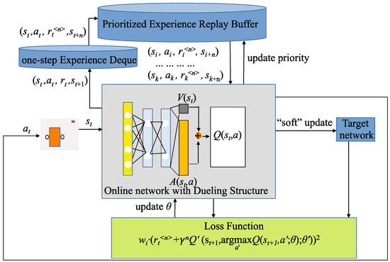
Figure 2. The diagram of the proposed n-step dueling DDQN with prioritized experience replay (PER-n₂D₃QN). The online network takes the environment state $s_t$ observed by the agent at time step t as input and separates into two streams at the last fully connected layer. After training with these parameters, a scalar stream $V\left(s_t\right)$ and a vector action advantage stream $A(s_t,a)$ are generated. Both streams are integrated to obtain the state-action value $Q(s_t,a)$, and the action with the maximum Q value is selected as the optimal action. After taking action $a_t$, the agent receives a reward, $r_t$, from the environment, and the environment transitions to state $s_{t+1}$. The experience ($s_t$, $a_t$, $r_t$, $s_{t+1}$) is stored in the one-step experience deque. During training, a batch of n-step prioritized experiences are sampled from the prioritized experience buffer, and the loss function is calculated to update the parameters of the online network. Subsequently, the TD target error is calculated to update the latest priority of the sampled prioritized experience in the buffer. The target network is updated from the online network using the “soft” update method.

When the agent observes its state $s_t$ in the environment at time step t, the online network selects and executes the optimal action $a_t$ with $\underset{a^{\prime }}{\mathrm{argmax}}Q(s_{t+1},a^{\prime };{\theta }_t)$. Subsequently, the agent receives an immediate reward, $r_t$, and the state transitions to a new one, $s_{t+1}$. Following this interaction, the one-step experience ($s_t$, $r_t$, $a_t$, $s_{t+1}$) is stored in the one-step experience deque, with a maximum capacity of n. Once this deque is filled with n experiences, these n consecutive experiences are used to generate an n-step experience ($s_t$, $r_t^{<n>}$, $a_t$, $s_{t+n}$). The notation $r_t^{<n>}$ represents the discounted accumulated rewards of subsequent n-step actions starting from time step t, calculated as $r_t^{<n>}$ = ${\sum }_{k=0}^{n-1}{\gamma }^k{r}_{t+k}$, where $s_{t+n}$ is the state at time step $t+n$. The n-step experience ($s_t$, $r_t^{<n>}$, $a_t$, $s_{t+n}$) is then stored in the prioritized experience buffer. To maintain a length of n consecutive experiences in the one-step experience deque, the earliest experience is removed from the end of the deque when a new experience is added from the top.

3.5. Exploration Policy

To facilitate learning, the agent should prioritize exploration during the early stages of training to gather more information and identify relationships between different states and actions. As training progresses, the agent should transition to exploiting learned knowledge, taking the action with $\underset{a^{\prime }}{\mathrm{argmax}}Q(s_t,a^{\prime };\theta )$.

In both the original DQN and DDQN algorithms, the agent utilizes the $ϵ$-greedy policy [11], choosing the action $\underset{a^{\prime }}{\mathrm{argmax}}Q(s_t,a^{\prime };\theta )$ with a probability of $1-ϵ$ and opting for a random action with a probability of $ϵ$[37,38]. The initial value of $ϵ$ is set to 1, and it decays at a rate of 0.99 per episode until reaching the minimum value of ${ϵ}_{min}$, which is adjusted to 0.01 to mitigate the impact of exploration on the results during the experiment [39]. The $ϵ$-greedy policy can be expressed as follows:

$$\begin{array}{c}a=\left\{\begin{array}{cc}\underset{a^{\prime }}{\mathrm{argmax}}Q(s_t,a^{\prime };\theta )\hfill & \mathrm{if}c>ϵ\hfill \\ \mathrm{random}\mathrm{action}\hfill & \mathrm{otherwise},\hfill \end{array}\right.\hfill \end{array}$$

(22)

where c is a random value from a uniform distribution in $\left[0,1\right]$.

While the $ϵ$-greedy strategy continues exploration during the entire learning process, it may lead to resource wastage, especially when a good estimation of certain actions is already available and further exploration is unnecessary. To address this limitation, this paper introduces a noisy network. It is a neural network whose weights and biases are perturbed by a parametric noise function to enhance the agent’s exploration efficiency, imposing an exploration noise onto the outputted Q-values. These parameters are updated using gradient descent [22], making agents more efficient in exploring environments and aiding in discovering meaningful exploration strategies to solve complex tasks.

In a neural network with p inputs and q outputs, the linear layer can be expressed as follows:

$$\begin{array}{c}y=\omega ·x+b,\hfill \end{array}$$

(23)

where $x\in {\mathbb{R}}^p$ is the input of the layer, $y\in {\mathbb{R}}^q$ is the output of the layer, and the weight matrix $\omega \in {\mathbb{R}}^{q\times p}$ and the bias $b\in {\mathbb{R}}^q$ need to be learned and updated. In the noisy network, $\omega$ is replaced with ${\mu }_{\omega }+{\sigma }_{\omega }\odot {\epsilon }_{\omega }$ and b with ${\mu }_b+{\sigma }_b\odot {\epsilon }_b$, where ${\mu }_{\omega }\in {\mathbb{R}}^{q\times p}$, ${\mu }_b\in {\mathbb{R}}^q$, ${\sigma }_{\omega }\in {\mathbb{R}}^{q\times p}$, ${\sigma }_b\in {\mathbb{R}}^q$. ${\mu }_{\omega }$, ${\mu }_b$, ${\sigma }_{\omega }$, and ${\sigma }_b$ need to be learned and updated in the noisy network using gradient descent. ${\epsilon }_{\omega }\in {\mathbb{R}}^{q\times p}$ and ${\epsilon }_b\in {\mathbb{R}}^q$ are random noise variables. In the noisy network, the linear layer with p inputs and q outputs is depicted in Figure 3.

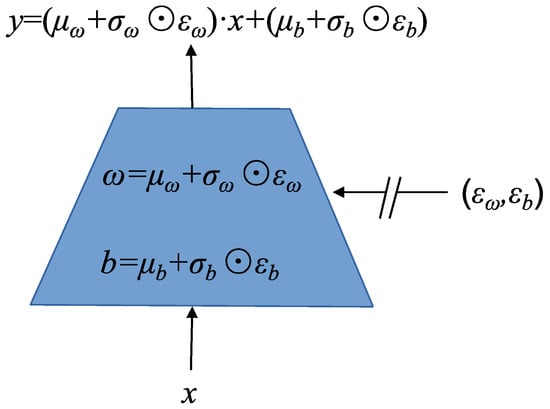
Figure 3. The linear layer structure of the noisy network, where ${\mu }_{\omega }\in {\mathbb{R}}^{q\times p}$, ${\mu }_b\in {\mathbb{R}}^q$, ${\sigma }_{\omega }\in {\mathbb{R}}^{q\times p}$, and ${\sigma }_b\in {\mathbb{R}}^q$ are the learnable parameters of the noisy network. ${\epsilon }_{\omega }\in {\mathbb{R}}^{q\times p}$ and ${\epsilon }_b\in {\mathbb{R}}^q$ are random noise variables. ⊙ represents the multiplication of the corresponding elements in the matrix. The output of the noisy layer is $y=({\mu }_{\omega }+{\sigma }_{\omega }\odot {\epsilon }_{\omega })·x+({\mu }_b+{\sigma }_b\odot {\epsilon }_b)$.

Factorized Gaussian noise is introduced to generate the random noise variables ${\epsilon }_{\omega }$ and ${\epsilon }_b$. To produce a matrix ${\epsilon }_{\omega }\in {\mathbb{R}}^{q\times p}$, one vector ${\epsilon }_q$ with q Gaussian random variables needs to be multiplied by the other vector ${\epsilon }_p$ with p random Gaussian variables. Subsequently, a total of q + p Gaussian variables are needed. The elements ${\epsilon }_{\omega (i,j)}$ in ${\epsilon }_{\omega }$ and ${\epsilon }_{b\left(i\right)}$ in ${\epsilon }_b$ can be generated as follows:

$$\begin{array}{cc}{\epsilon }_{\omega (i,j)}\hfill & =f\left({\epsilon }_{q\left(i\right)}\right)f\left({\epsilon }_{p\left(j\right)}\right)\hfill \end{array}$$

(24)

$$\begin{array}{cc}{\epsilon }_{b\left(i\right)}\hfill & =f\left({\epsilon }_{q\left(i\right)}\right),\hfill \end{array}$$

(25)

where the function $f\left(m\right)=\mathrm{sgn}\left(m\right)\sqrt{\left|m\right|}$. Although ${\epsilon }_{\omega }$ and ${\epsilon }_b$ are Gaussian random variables, their values are fixed in the neural network. All parameters ${\epsilon }_{q\left(i\right)}$ and ${\epsilon }_{p\left(j\right)}$ conform to a Gaussian distribution as ${\epsilon }_{q\left(i\right)}$, ${\epsilon }_{p\left(j\right)}\sim$$N(0,1)$. For factorized noisy networks, ${\mu }_{\omega }$ and ${\mu }_b$ are initialized by random samples from independent uniform distributions, i.e., ${\mu }_{\omega }$, ${\mu }_b\sim [-\frac{1}{\sqrt{p}},\frac{1}{\sqrt{p}}]$. All the elements in ${\sigma }_{\omega }$, ${\sigma }_b$ are set to $\frac{0.5}{\sqrt{p}}$ based on suggestions from prior research [22].

When replacing the traditional linear layers with noisy layers in the n-step DDQN, the online network is described as $Q(s,a,\epsilon ;\zeta$), where $\epsilon$ is the random variable, and $\zeta$ is the learnable parameters of the online network. Similarly, the target network is expressed as $Q^{\prime }(s,a,{\epsilon }^{\prime };{\zeta }^{\prime }$). The loss function of the n-step DDQN with noise, $L{\left(\xi \right)}_{Noisy}$, can be expressed as follows:

$$\begin{array}{c}L{\left(\xi \right)}_{Noisy}={\mathbb{E}}_{\cancel{\underset{=}{\subset }},{\cancel{\underset{=}{\subset }}}^{\prime }}[{\mathbb{E}}_{~}[\sum _{k=0}^{n-1}{\gamma }^k{r}_{t+k}+{\gamma }^n{Q}^{\prime }(s_{t+1},\underset{a^{\prime }}{\mathrm{argmax}}Q(s_{t+1},a^{\prime },\epsilon ;\zeta ),{\epsilon }^{\prime };{\zeta }^{\prime }))-Q(s,a,\epsilon ;\zeta ){]}^2].\hfill \end{array}$$

(26)

4. PER-n₂D₃QN for Mobile Robot Navigation

4.1. Action Space

The DDQN algorithm is one of the value-based RL algorithms that can only be utilized in discrete action spaces. Therefore, the movements of mobile robots must be discretized. Based on prior research [40,41] and our experimental attempts, the action space can be discretized into five actions: a large left turn, a small left turn, a forward motion, a small right turn, and a large right turn. Each action consists of two dimensions: line velocity and regular velocity. The linear velocity of the mobile robot remains constant at $v_0=0.15$ m/s, while the angular velocity varies for each action, denoted by $(2w_0,w_0,0,-w_0,-2w_0)$, where the lower angular velocity $w_0=0.75$ rad/s. Therefore, the action space can be represented as follows:

$$\begin{array}{c}A=\left\{(v_0,2w_0),(v_0,w_0),(v_0,0),(v_0,-w_0),(v_0,-2w_0)\right\}.\hfill \end{array}$$

(27)

4.2. State Space

The state represents the environmental information perceived by the agent, directly affecting its decisions during learning. In achieving efficient and collision-free navigation for the mobile robot in complex environments, designing the state space also plays an important role. The DDQN is typically more suitable for discrete state spaces, leveraging Q values within a discrete action space to optimize the policy [42].

Our experiments use the Waffle model of the TurtleBot3 mobile robot, a popular open-source platform designed for education, research, and hobbyist use and specifically tailored to work with the robot operating system (ROS). The Waffle model, equipped with sensors, employs a laser beam to detect obstacles in a 360° direction, calculating distances based on the return time and providing a comprehensive view of the surroundings. During robot navigation, the real-time state information is perceived through a LIDAR sensor and an odometer [43]. The LIDAR sensor captures distance and heading information between the robot, goal, and obstacles, while the odometer supplies the robot’s position. The efficiency of the algorithm is greatly influenced by the size of the state space. If the state space is too small, the algorithm will have low accuracy. Otherwise, it will take too much more time for training and convergence.

After multiple attempts and referencing a related paper [43], our implementation utilizes only the distances from the LIDAR sensor at 24 equidistant points, reducing the state space to 28. The state space is defined as

$$\begin{array}{c}S=[{d_L}^T,\varphi ,d_g,d_o,n],\hfill \end{array}$$

(28)

where ${d_L}^T$ represents 24 distances to the obstacles uniformly scanned by the LIDAR sensor and is expressed as ${d_L}^T=[d_0,d_1,d_2\dots \dots d_{23}]$. $\varphi$ is the heading angle between the mobile robot and the target. $d_g$ is the distance to the goal. $d_o$ is the minimum distance to the nearest obstacle detected by the LIDAR sensor, and n is the index corresponding to the minimum distance, which is used to calculate the angle of the nearest obstacle relative to the robot. The acquisition of the mobile robot state is illustrated in Figure 4.

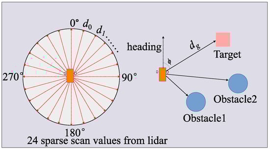
Figure 4. The acquisition of the mobile robot state, where $\varphi$ and $d_g$ represent the heading and distance between the robot and the goal.

4.3. Target-Oriented Reward Function

In the context of RL, the reward function serves the purpose of guiding the agent to learn the value of different actions with a given state [44]. In the domain of autonomous navigation for mobile robots, a straightforward method involves utilizing sparse rewards, where positive rewards are only received by the agent when reaching the goal, while negative rewards are given if it collides with an obstacle. This can result in slower or erratic learning. However, in complicated environments with abundant dense or dynamic obstacles, navigating to the target becomes exceedingly challenging for the mobile robot. Operating in such environments with sparse rewards often leads to the mobile robot becoming disoriented or immobilized. Fortunately, reward shaping provides the agent with a smoother and denser form of non-sparse reward, enabling the agent to receive more intermediate reward signals during task execution. This offers more guidance and expedites the learning process [45].

In this paper, a novel target-oriented reshaping reward function is proposed, which adjusts rewards based on factors like the distance and direction between the robot and the target and the distance between the robot and the obstacles. For instance, if the mobile robot is closer to the target, a higher reward might be given to incentivize the mobile robot to reach the goal more quickly. However, if the mobile robot is closer to the obstacle, it may receive a lower reward as a penalty to prevent it from colliding with the obstacle. This target-oriented reshaping reward function encompasses three scenarios. Firstly, if the minimum distance between the mobile robot and the obstacle is less than $l_a$, it is deemed a collision, and the agent receives a reward of −500. Secondly, when the current distance between the mobile robot and the target is less than $l_b$, the robot is considered to have successfully reached the goal, and the agent is rewarded with 1000 [46]. Otherwise, the reward is the sum of $r_1$ and $r_2$, where $r_1$ is calculated based on the angle of the current action and the current distance to the target. $r_2$ is set to −5 when the minimum distance between the mobile robot and the obstacle is less than 0.5; otherwise, $r_2$ is set to 1. The reward function can be expressed as follows:

$$\begin{array}{c}r=\left\{\begin{array}{cc}-500\hfill & \mathrm{if}\mathrm{collision}\hfill \\ 1000\hfill & \mathrm{if}\mathrm{goal}\mathrm{reached}\hfill \\ r_1+r_2\hfill & \mathrm{otherwise}.\hfill \end{array}\right.\hfill \end{array}$$

(29)

To facilitate result evaluation and comparison, the DQN, DDQN, and PER-n₂D₃QN algorithms share this same reward function [41]. In summary, the pseudocode of the proposed PER-nD₃QN is outlined in Algorithm 1.

Algorithm 1 Prioritized Experience Reply Noisy n-step Dueling DDQN algorithm

1: Set the state dimension to 28, the size of the action space to 5, the capacity of the deque D to $n=5$, and the parameters mini-batch size k, learning rate $\eta$, prioritization parameters $\iota$ and $\varrho$, noisy network parameters ${\mu }_{\omega }$, ${\mu }_b\sim [-\frac{1}{\sqrt{28}},\frac{1}{\sqrt{28}}]$, and all elements in ${\sigma }_{\omega }$, ${\sigma }_b$ to $\frac{0.5}{\sqrt{28}}$. 2: Initialize priority $p_1$ = 1, learning rate = $\eta$, and dueling noisy online network Q and target network $Q^{\prime }$ with parameters $\xi$ and ${\xi }^{\prime }$. 3: for $episode=1\to M$ do 4:     Initialize environment state $s_1$ 5:     for $t=1\to T$ do 6:         Sample a noisy network $\xi \sim \epsilon$ 7:         Choose action $a_t$ = $\underset{a}{\mathrm{argmax}}Q(s_t,a,\epsilon ;\xi )$ 8:         Take action $a_t$, observe $r_t$, $s_{t+1}$ 9:         Store experience ($s_t$, $r_t$, $a_t$, $s_{t+1}$) in D 10:         if Length of D == n then 11:            Store n-step experience ($s_t$, $r_t^{<n>}$, $a_t$, $s_{t+n}$) in a buffer with initial priority $p_1$ 12:         end if 13:         for $j=1\to k$ do 14:            Sample experience j based on the priority $P\left(j\right)$ shown in Equation (18) 15:            Sample noisy variables $\epsilon$ and ${\epsilon }^{\prime }$ for Q and $Q^{\prime }$ 16:            $y_j\leftarrow r_t^{<n>}$+${\gamma }^n{Q}^{\prime }(s_{j+n},\underset{a^{\prime }}{\mathrm{argmax}}Q(s_{j+n},a^{\prime },\epsilon ;\xi );{\epsilon }^{\prime };{\xi }^{\prime })$ 17:            Compute the TD target error ${\delta }_j$ 18:            Compute the IS weight $w_j=W_j/{\max }_i{W}_i$ by Equation (19) 19:            Update parameters with ${\theta }_{j+1}={\theta }_j-\eta ·w_j·{\delta }_j{\nabla }_{{\theta }_j}Q(s_j,a_j;{\theta }_j)$ 20:            Update priority $p_j=\left|{\delta }_j\right|+\rho$ for experience j 21:         end for 22:         “soft” update target network $Q^{\prime }$ 23:         $s_j\leftarrow s_{j+n}$ 24:     end for 25: end for

5. Numerical Experiments and Results

5.1. Experimental Settings

To evaluate the performance of the proposed algorithm PER-n₂D₃QN, we conducted experiments simulating mobile robot navigation tasks across three scenarios using the DQN, DDQN, and PER-n₂D₃QN methods (the codes are available at https://github.com/iAerialRobo (accessed on 1 January 2024)). The experiments were conducted on a laptop with an 8 GB NVIDIA GTX4060 GPU and 16 GB RAM employing the open-source robot operating system (ROS) [47,48] and open-source 3D simulator Gazebo [49]. The model is implemented in Python 3.8.10 using PyTorch 1.11, with experiment-specific parameters detailed in Table 1.

Table 1. Experiment hyper-parameters.

Parameters	Values	Remark
$\gamma$	0.99	Discount factor
M	200,000	Size of experience replay memory
D	200,000	Size of SumTree in PER memory
BATCH_SIZE	64	Size of sampled batch
$\iota$	0.6	Extent of prioritization
$\varrho$	0.4	Extent to correct bias of prioritization sampling
$\tau$	0.005	Update magnitude of target network
$\eta$	0.001	Learning rate
n	5	n-step in TD method
$l_a$	0.13 m	Threshold of collision
$l_b$	0.2 m	Threshold of reaching goal
$v_0$	0.15 m/s	Linear velocity of mobile robot
$w_0$	0.75 rad/s	Rotational speed of mobile robot

The agent employed is the Waffle model of the TurtleBot3 mobile robot, navigating three distinct scenarios depicted in Figure 5. In scenario 1, as shown in Figure 5a, a static environment with simple obstacles is presented, featuring four cylindrical obstacles around the mobile robot. Furthermore, the area of the entire closed area is 4 × 4 m², and the radius of the cylindrical obstacle in the area is 0.15 m. Scenario 2 in Figure 5b retains a static setting but introduces a more complex environment with numerous rectangular obstacles. In addition, the area of the entire closed area is 5 × 5 m², and the length of the rectangular obstacle in the area is 1 m, while the width and height are the same as those of the outer wall. Lastly, scenario 3 in Figure 5c incorporates two dynamic cylindrical obstacles with a radius of 0.12 m, moving with a line velocity of 0.5 m/s. In these three scenarios, all the target positions are generated randomly.

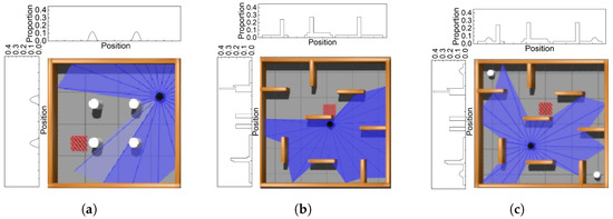
Figure 5. Static and dynamic simulation scenarios, where the black point represents the mobile robot, and the red square represents the target. (a) Scenario 1 with static obstacles. (b) Scenario 2 with static obstacles. (c) Scenario 3 with dynamic obstacles.

5.2. Quantitative Analysis of Simulation Environment

In scientific research and engineering design, quantitative analysis provides comprehensive and robust support. To better illustrate the complexity variety between different scenarios in the simulation environment, we projected obstacles onto the X- and Y-axes and quantitatively analyzed environmental complexity based on the proportion of obstacle projections throughout the environment with the removal of the width of the outermost wall. The analysis results are also depicted in Figure 5.

In scenario 1, the projection distribution of obstacles on the x- and y-axes is relatively sparse, with only two distribution areas with an obstacle, and the maximum projection proportion on the x-axes is only 0.0811 and the same with the y-axes. Additionally, the area of obstacles accounts for 0.516% of the entire simulation environment area. In scenario 2, the projection distribution of obstacles on the x- and y-axes has significantly increased. Furthermore, the maximum projection proportions on the x- and y-axes are 0.2766 and 0.4255, respectively. In addition, the obstacles encompass 5.432% of the total simulation environment area. Scenario 3 adds dynamically moving obstacles based on scenario 2, and we only show the obstacle projection distribution in the initial state. As the positions of dynamic obstacles change, their projected positions on the x- and y-axes change in real time. When calculating the proportion of the obstacle area to the total area, to distinguish the difference between dynamic obstacles and static obstacles, we use the relative value of the linear speed of the dynamic obstacle compared to that of the mobile robot as the weight, and the product of this weight and the area of the dynamic obstacles is used as the final area of the dynamic obstacle. Thus, the obstacles encompass 19.47% of the total simulation environment area. The quantitative analysis of simulation environment complexity allows for a more accurate description of environmental complexity and provides deeper insights into the performance of the three algorithms.

5.3. Results and Discussion

To assess the performance of the DQN, DDQN, and proposed PER-n₂D₃QN methods across three scenarios, we analyze the average score (AS) and success rate (SR). Figure 6 depicts the performance comparison of the three algorithms after 10 training trials in scenario 1, with each trial comprising 1100 episodes. Table 2 details the average reward and success rate statistics. DQN achieves an average score of 828.18 with a standard deviation (SD) of 248.05, and it increases to 1049.51 for the DDQN, coupled with a standard deviation of 198.96. Remarkably, PER-n₂D₃QN reaches a substantially higher average score of 3384.88 with a standard deviation of 224.69. The average success rate follows a similar trend, improving from 62.74% with a standard deviation of 5.88% for the DQN to 63.92% with a standard deviation of 4.32% for the DDQN and, finally, to 98.91% with a standard deviation of 3.41% for PER-n₂D₃QN. In this simpler static scenario 1, there is marginal improvement in the average score between the DQN and DDQN, with little difference in the success rate. However, PER-n₂D₃QN outperforms both the DQN and DDQN significantly in terms of both the average score and success rate.

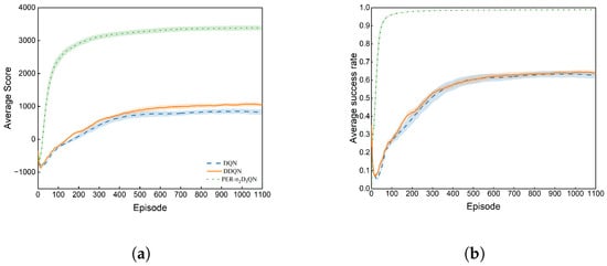
Figure 6. Experimental results in scenario 1 when trained 1100 episodes (shadowed color: Standard Error). (a) Average score over 10 trials. (b) Average success rate over 10 trials.

Table 2. Experimental results when trained for 1100 episodes in scenario 1.

Algorithm	Indicator	Trial 1	Trial 2	Trial 3	Trial 4	Trial 5	Trial 6	Trial 7	Trial 8	Trial 9	Trial 10	Average	SD
DQN	SR	58.41%	67.05%	62.97%	69.72%	61.12%	53.54%	55.75%	67.55%	70.60%	60.74%	62.74%	5.88%
	AS	678.66	1040.13	771.10	1223.60	709.68	475.56	509.12	1014.16	1055.19	804.62	828.18	248.05
DDQN	SR	63.69%	69.07%	65.22%	63.95%	68.93%	63.75%	65.25%	61.03%	53.73%	64.59%	63.92%	4.32%
	AS	1002.67	1290.22	1072.25	1080.94	1340.69	1006.20	1097.82	909.00	619.17	1076.14	1049.51	198.96
PER-n2D3QN	SR	98.95%	99.05%	99.02%	99.12%	98.26%	99.35%	98.34%	98.98%	99.06%	98.99%	98.91%	3.41%
	AS	3394.45	3720.51	3503.49	3466.41	2981.46	3449.78	3036.66	3327.22	3415.28	3553.57	3384.88	224.69

Next, we evaluated the performance of the three algorithms in scenario 2, with 1600 episodes per trial and 10 repeated trials. Figure 7a and Figure 7b, respectively, illustrate the results for the average score and success rate, while Table 3 provides specific statistics. The DQN starts with an average score of −309.56 coupled with a standard deviation of 199.66, and it improves to −209.01 with a standard deviation of 244.97 for the DDQN. In contrast, PER-n₂D₃QN achieves a substantially increased average score of 2862.23, along with a standard deviation of 236.93. Additionally, the success rate of the DQN is a mere 2.97% with a standard deviation of 2.47%, improving to 15.08% with a standard deviation of 11.21% for the DDQN and eventually reaching 98.32% with a standard deviation of 3.83% for PER-n₂D₃QN. Similar to scenario 1, the DDQN performs better than the DQN in the more complex static scenario 2. The increment in the average score between the DQN and DDQN is 100.55, and the average success rate improves by 12.11%. However, the DDQN’s accuracy and stability remain relatively low. Conversely, PER-n₂D₃QN excels in scenario 2 with high accuracy and stability.

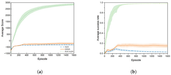
Figure 7. Experimental results in scenario 2 when trained for 1600 episodes (shadowed color: Standard Error). (a) Average score over 10 trials. (b) Average success rate over 10 trials.

Table 3. Experimental results when trained for 1600 episodes in scenario 2.

Algorithm	Indicator	Trial 1	Trial 2	Trial 3	Trial 4	Trial 5	Trial 6	Trial 7	Trial 8	Trial 9	Trial 10	Average	SD
DQN	SR	1.46%	5.79%	4.28%	3.73%	1.05%	2.93%	0.74%	0.14%	1.73%	7.88%	2.97%	2.47%
	AS	126.14	−468.26	−39.58	−378.76	−295.53	−354.15	−434.54	−357.35	−511.33	−382.24	−309.56	199.66
DDQN	SR	34.72%	9.05%	4.16%	9.04%	11.53%	25.60%	7.15%	10.95%	6.77%	31.85%	15.08%	11.21%
	AS	335.99	−336.34	−439.81	−243.87	−339.58	−134.19	−346.52	−308.70	−374.07	97.01	−209.01	244.97
PER-nD3QN	SR	98.39%	98.78%	97.45%	98.51%	98.21%	98.31%	97.96%	98.41%	98.48%	98.69%	98.32%	3.83%
	AS	2846.56	3060.75	2347.53	3108.40	2751.96	2946.01	2700.06	2861.52	2831.30	3168.20	2862.23	236.93

Finally, we evaluated the three methods in dynamic scenario 3, also with 10 trials, and each trial comprised 2000 episodes. Figure 8a and Figure 8b, respectively, show the results for the average score and success rate, with detailed statistics in Table 4. The DQN and DDQN perform poorly in scenario 3. Specifically, the DQN achieves a success rate of only 1.59% with a standard deviation of 0.85%, and the DDQN’s success rate rises to a mere 8.95% with a standard deviation of 4.52%. In contrast, PER-n₂D₃QN achieves a high average score of 2571.28 with a standard deviation of 108.20 and a success rate of 92.63% with a standard deviation of 0.93%. Although the DDQN outperformed DQN in dynamic scenario 3, with an improvement in the average score of 58.68 and a 7.36% increase in the average success rate, its accuracy and stability still lag behind those in scenario 2. On the other hand, PER-n₂D₃QN continued to excel in scenario 3, demonstrating high accuracy and stability.

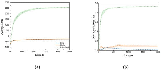
Figure 8. Experimental results in scenario 3 when trained for 2000 episodes (shadowed color: Standard Error). (a) Average score over 10 trials. (b) Average success rate over 10 trials.

Table 4. Experimental results when trained for 2000 episodes in scenario 3.

Algorithm	Indicator	Trial 1	Trial 2	Trial 3	Trial 4	Trial 5	Trial 6	Trial 7	Trial 8	Trial 9	Trial 10	Average	SD
DQN	SR	2.52%	1.18%	2.11%	2.98%	0.22%	1.53%	0.56%	1.24%	2.07%	1.49%	1.59%	0.85%
	AS	−307.24	−492.05	−428.13	−311.97	−370.97	62.36	−516.04	−315.77	−314.34	−248.65	−324.28	161.14
DDQN	SR	2.64%	3.83%	15.92%	10.92%	8.21%	13.86%	6.47%	6.46%	13.96%	7.20%	8.95%	4.52%
	AS	−441.57	−317.00	−268.187	−164.32	−376.43	−182.39	−260.03	−205.50	−294.43	−146.51	−265.63	95.30
PER-nD3QN	SR	91.27%	91.67%	94.20%	93.50%	92.13%	91.76%	92.49%	93.36%	92.89%	93.07%	92.63%	0.93%
	AS	2434.01	2489.42	2769.54	2695.33	2491.18	2571.50	2637.07	2541.79	2618.10	2464.87	2571.28	108.20

In the simpler static scenario 1, the average score increased by 222.52% and the success rate improved by 54.74% when comparing the proposed algorithm PER-n₂D₃QN with the DDQN. In the more complex static scenario 2, the average score increased by 1469.42%, and the success rate was enhanced by 551.99% when comparing the DDQN to PER-n₂D₃QN. In dynamic scenario 3, the average score rose by 1068.10%, and the success rate experienced a substantial 934.97% enhancement from the DDQN to PER-n₂D₃QN. In the detailed performance comparison of the DQN, DDQN, and PER-n₂D₃QN across the three scenarios, it is evident that the PER-n₂D₃QN method exhibits superior and stable performance in mobile robot navigation, particularly in complex static and dynamic scenarios. The method demonstrates remarkable improvement in the average score and success rate compared to the DQN and DDQN, especially in scenarios involving static obstacles and dynamic elements. Additionally, the visualized path using the policy trained by the PER-n₂D₃QN method in scenario 1 within an episode is depicted in in Figure 9. Similarly, the paths in scenarios 2 and 3 are shown in Figure 10 and Figure 11, respectively. In each episode, the mobile robot can take up to 300 steps. However, if a collision occurs, the current episode terminates. Upon reaching the current target, the mobile robot will continue to search for the next new target starting from the current position until it has taken 300 steps.

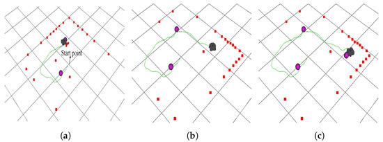
Figure 9. The whole path conducted by the PER-n₂D₃QN algorithm in scenario 1 within one episode. The red square symbol represents the obstacles detected by the radar, the purple sphere represents the target point, and the green curve represents the path taken by the robot within an episode. (a) Case 1. (b) Case 2. (c) Case 3.

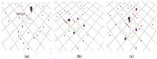
Figure 10. The whole path conducted by the PER-n₂D₃QN algorithm in scenario 2 within one episode. The red square symbol represents the obstacles detected by the radar, the purple sphere represents the target point, and the green curve represents the path taken by the robot within an episode. (a) Case 1. (b) Case 2. (c) Case 3.

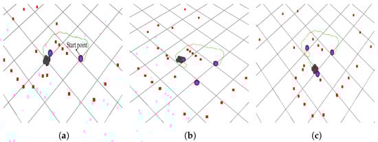
Figure 11. The whole path conducted by the PER-n₂D₃QN algorithm in scenario 3 within one episode. The red square symbol represents the obstacles detected by the radar, the purple sphere represents the target point, and the green curve represents the path taken by the robot within an episode. (a) Case 1. (b) Case 2. (c) Case 3.

6. Conclusions

This paper presents an advanced approach to autonomous navigation for mobile robots termed PER-n₂D₃QN, which is an extension of the DDQN. It significantly enhances the performance of autonomous navigation, including the average score, path efficiency, and accuracy, by incorporating prioritized experience replay, a noisy network, n-step learning, and a dueling network structure into the DDQN. Furthermore, an effective target-oriented reshaping reward function is employed to expedite learning, coupled with useful techniques, including a target “soft” update and a gradient clipping mechanism, to improve the stability and robustness of learning. These improvements boost the efficiency of experience replay, promote exploration, and deliver a more precise Q-value estimate, thereby significantly enhancing the performance of autonomous navigation for mobile robots. In addition, to further capture the complexity of the simulation environment, this paper presents a comprehensive quantitative analysis of the simulation environment for the first time. Subsequently, to validate the proposed algorithm, we conducted extensive experiments using the DQN, DDQN, and PER-n₂D₃QN on the ROS and Gazebo platforms for mobile robot autonomous navigation tasks.

The trained models were assessed across three distinct scenarios: two static simulation settings and one dynamic simulation setting. A comparative analysis of performance metrics, including the average reward and success rate, reveals that PER-n₂D₃QN exhibits remarkable improvements and enhanced robustness, particularly across all three scenarios. Although the experiment focuses on wheeled robots, this approach can extend to various types of mobile robots, including legged robots and aerial robots, as it learns directly from sensor inputs and does not rely on the type or model of the robots. Future research will delve into autonomous navigation for mobile robots in more complex tasks involving coordination and collaboration among multiple agents to improve traffic flow efficiency and safety and reduce training time.

References

- Liu, Z.; Zhai, Y.; Li, J.; Wang, G.; Miao, Y.; Wang, H. Graph Relational Reinforcement Learning for Mobile Robot Navigation in Large-Scale Crowded Environments. IEEE Trans. Intell. Transp. Syst. 2023, 24, 8776–8787. [Google Scholar] [CrossRef]
- Lee, H.; Ho, H.W.; Zhou, Y. Deep Learning-based monocular obstacle avoidance for unmanned aerial vehicle navigation in tree plantations: Faster region-based convolutional neural network approach. J. Intell. Robot. Syst. 2021, 101, 1–18. [Google Scholar] [CrossRef]
- Müller, C.J.; van Daalen, C.E. Map point selection for visual SLAM. Robot. Auton. Syst. 2023, 167, 104485. [Google Scholar] [CrossRef]
- Shi, H.; Shi, L.; Xu, M.; Hwang, K.S. End-to-end navigation strategy with deep reinforcement learning for mobile robots. IEEE Trans. Ind. Inform. 2019, 16, 2393–2402. [Google Scholar] [CrossRef]
- Temeltas, H.; Kayak, D. SLAM for robot navigation. IEEE Aerosp. Electron. Syst. Mag. 2008, 23, 16–19. [Google Scholar] [CrossRef]
- Quan, H.; Li, Y.; Zhang, Y. A novel mobile robot navigation method based on deep reinforcement learning. Int. J. Adv. Robot. Syst. 2020, 17, 1729881420921672. [Google Scholar] [CrossRef]
- Kaufmann, E.; Bauersfeld, L.; Loquercio, A.; Müller, M.; Koltun, V.; Scaramuzza, D. Champion-level drone racing using deep reinforcement learning. Nature 2023, 620, 982–987. [Google Scholar] [CrossRef]
- LeCun, Y.; Bengio, Y.; Hinton, G. Deep learning. Nature 2015, 521, 436–444. [Google Scholar] [CrossRef] [PubMed]
- Peng, X.; Chen, R.; Zhang, J.; Chen, B.; Tseng, H.W.; Wu, T.L.; Meen, T.H. Enhanced Autonomous Navigation of Robots by Deep Reinforcement Learning Algorithm with Multistep Method. Sensor Mater. 2021, 33, 825–842. [Google Scholar] [CrossRef]
- Kaelbling, L.P.; Littman, M.L.; Moore, A.W. Reinforcement learning: A survey. J. Artif. Intell. Res. 1996, 4, 237–285. [Google Scholar] [CrossRef]
- Sutton, R.S.; Barto, A.G. Reinforcement Learning: An Introduction; MIT Press: Cambridge, MA, USA, 2018. [Google Scholar]
- Zhou, Y.; Ho, H.W. Online robot guidance and navigation in non-stationary environment with hybrid Hierarchical Reinforcement Learning. Eng. Appl. Artif. Intell. 2022, 114, 105152. [Google Scholar] [CrossRef]
- Mnih, V.; Kavukcuoglu, K.; Silver, D.; Rusu, A.A.; Veness, J.; Bellemare, M.G.; Graves, A.; Riedmiller, M.; Fidjeland, A.K.; Ostrovski, G.; et al. Human-level control through deep reinforcement learning. Nature 2015, 518, 529–533. [Google Scholar] [CrossRef]
- Yuan, Y.; Yu, Z.L.; Gu, Z.; Yeboah, Y.; Wei, W.; Deng, X.; Li, J.; Li, Y. A novel multi-step Q-learning method to improve data efficiency for deep reinforcement learning. Knowl.-Based Syst. 2019, 175, 107–117. [Google Scholar] [CrossRef]
- Choi, J.; Park, K.; Kim, M.; Seok, S. Deep Reinforcement Learning of Navigation in a Complex and Crowded Environment with a Limited Field of View. In Proceedings of the 2019 IEEE International Conference on Robotics and Automation (ICRA), Montreal, QC, Canada, 20–24 May 2019; pp. 5993–6000. [Google Scholar] [CrossRef]
- Van Hasselt, H.; Guez, A.; Silver, D. Deep reinforcement learning with double q-learning. In Proceedings of the AAAI Conference on Artificial Intelligence, Phoenix, AZ, USA, 12–17 February 2016; Volume 30. [Google Scholar]
- Levine, S.; Finn, C.; Darrell, T.; Abbeel, P. End-to-end training of deep visuomotor policies. J. Mach. Learn. Res. 2016, 17, 1334–1373. [Google Scholar]
- Zhu, W.; Hayashibe, M. A Hierarchical Deep Reinforcement Learning Framework With High Efficiency and Generalization for Fast and Safe Navigation. IEEE Trans. Ind. Electron. 2023, 70, 4962–4971. [Google Scholar] [CrossRef]
- Hessel, M.; Modayil, J.; Van Hasselt, H.; Schaul, T.; Ostrovski, G.; Dabney, W.; Horgan, D.; Piot, B.; Azar, M.; Silver, D. Rainbow: Combining improvements in deep reinforcement learning. In Proceedings of the AAAI Conference on Artificial Intelligence, New Orleans, LA, USA, 2–7 February 2018; Volume 32. [Google Scholar]
- Schaul, T.; Quan, J.; Antonoglou, I.; Silver, D. Prioritized experience replay. arXiv 2015, arXiv:1511.05952. [Google Scholar]
- Li, T.; Yang, D.; Xie, X. Prioritized experience replay based reinforcement learning for adaptive tracking control of autonomous underwater vehicle. Appl. Math. Comput. 2023, 443, 127734. [Google Scholar] [CrossRef]
- Fortunato, M.; Azar, M.G.; Piot, B.; Menick, J.; Osband, I.; Graves, A.; Mnih, V.; Munos, R.; Hassabis, D.; Pietquin, O.; et al. Noisy networks for exploration. arXiv 2017, arXiv:1706.10295. [Google Scholar]
- Hernandez-Garcia, J.F.; Sutton, R.S. Understanding multi-step deep reinforcement learning: A systematic study of the DQN target. arXiv 2019, arXiv:1901.07510. [Google Scholar]
- Wang, Z.; Schaul, T.; Hessel, M.; Hasselt, H.; Lanctot, M.; Freitas, N. Dueling network architectures for deep reinforcement learning. In Proceedings of the International Conference on Machine Learning (PMLR), New York, NY, USA, 20–22 June 2016; pp. 1995–2003. [Google Scholar]
- Gök, M. Dynamic path planning via Dueling Double Deep Q-Network (D3QN) with prioritized experience replay. Appl. Soft Comput. 2024, 158, 111503. [Google Scholar] [CrossRef]
- Motlagh, O.; Nakhaeinia, D.; Tang, S.H.; Karasfi, B.; Khaksar, W. Automatic navigation of mobile robots in unknown environments. Neural Comput. Appl. 2014, 24, 1569–1581. [Google Scholar] [CrossRef]
- Li, H.; Qin, J.; Liu, Q.; Yan, C. An Efficient Deep Reinforcement Learning Algorithm for Mapless Navigation with Gap-Guided Switching Strategy. J. Intell. Robot. Syst. 2023, 108, 43. [Google Scholar] [CrossRef]
- Chen, Y.F.; Everett, M.; Liu, M.; How, J.P. Socially aware motion planning with deep reinforcement learning. In Proceedings of the 2017 IEEE/RSJ International Conference on Intelligent Robots and Systems (IROS), Vancouver, BC, Canada, 24–28 September 2017; pp. 1343–1350. [Google Scholar]
- Din, A.; Ismail, M.Y.; Shah, B.; Babar, M.; Ali, F.; Baig, S.U. A deep reinforcement learning-based multi-agent area coverage control for smart agriculture. Comput. Electr. Eng. 2022, 101, 108089. [Google Scholar] [CrossRef]
- Singh, S.; Jaakkola, T.; Littman, M.L.; Szepesvári, C. Convergence results for single-step on-policy reinforcement-learning algorithms. Mach. Learn. 2000, 38, 287–308. [Google Scholar] [CrossRef]
- Watkins, C.J.; Dayan, P. Q-learning. Mach. Learn. 1992, 8, 279–292. [Google Scholar] [CrossRef]
- Peng, B.; Sun, Q.; Li, S.E.; Kum, D.; Yin, Y.; Wei, J.; Gu, T. End-to-end autonomous driving through dueling double deep Q-network. Automot. Innov. 2021, 4, 328–337. [Google Scholar] [CrossRef]
- Cao, X.; Wan, H.; Lin, Y.; Han, S. High-value prioritized experience replay for off-policy reinforcement learning. In Proceedings of the 2019 IEEE 31st International Conference on Tools with Artificial Intelligence (ICTAI), Portland, OR, USA, 4–6 November 2019; pp. 1510–1514. [Google Scholar]
- Neal, R.M. Annealed importance sampling. Stat. Comput. 2001, 11, 125–139. [Google Scholar] [CrossRef]
- Horgan, D.; Quan, J.; Budden, D.; Barth-Maron, G.; Hessel, M.; Van Hasselt, H.; Silver, D. Distributed prioritized experience replay. arXiv 2018, arXiv:1803.00933. [Google Scholar]
- Kobayashi, T.; Ilboudo, W.E.L. T-soft update of target network for deep reinforcement learning. Neural Netw. 2021, 136, 63–71. [Google Scholar] [CrossRef]
- Xue, X.; Li, Z.; Zhang, D.; Yan, Y. A deep reinforcement learning method for mobile robot collision avoidance based on double dqn. In Proceedings of the 2019 IEEE 28th International Symposium on Industrial Electronics (ISIE), Vancouver, BC, Canada, 12–14 June 2019; pp. 2131–2136. [Google Scholar]
- Ladosz, P.; Weng, L.; Kim, M.; Oh, H. Exploration in deep reinforcement learning: A survey. Inf. Fusion 2022, 85, 1–22. [Google Scholar] [CrossRef]
- Wang, D.; Deng, H.; Pan, Z. Mrcdrl: Multi-robot coordination with deep reinforcement learning. Neurocomputing 2020, 406, 68–76. [Google Scholar] [CrossRef]
- Jaradat, M.A.K.; Al-Rousan, M.; Quadan, L. Reinforcement based mobile robot navigation in dynamic environment. Robot. Comput.-Integr. Manuf. 2011, 27, 135–149. [Google Scholar] [CrossRef]
- Marchesini, E.; Farinelli, A. Discrete deep reinforcement learning for mapless navigation. In Proceedings of the 2020 IEEE International Conference on Robotics and Automation (ICRA), Paris, France, 31 May–31 August 2020; pp. 10688–10694. [Google Scholar]
- Tai, L.; Paolo, G.; Liu, M. Virtual-to-real deep reinforcement learning: Continuous control of mobile robots for mapless navigation. In Proceedings of the 2017 IEEE/RSJ International Conference on Intelligent Robots and Systems (IROS), Vancouver, BC, Canada, 24–28 September 2017; pp. 31–36. [Google Scholar]
- Li, W.; Yue, M.; Shangguan, J.; Jin, Y. Navigation of Mobile Robots Based on Deep Reinforcement Learning: Reward Function Optimization and Knowledge Transfer. Int. J. Control. Autom. Syst. 2023, 21, 563–574. [Google Scholar] [CrossRef]
- Liu, L.; Dugas, D.; Cesari, G.; Siegwart, R.; Dubé, R. Robot Navigation in Crowded Environments Using Deep Reinforcement Learning. In Proceedings of the 2020 IEEE/RSJ International Conference on Intelligent Robots and Systems (IROS), Las Vegas, NV, USA, 24 October 2020–24 January 2021; pp. 5671–5677. [Google Scholar] [CrossRef]
- Ng, A.Y.; Harada, D.; Russell, S. Policy invariance under reward transformations: Theory and application to reward shaping. In Proceedings of the ICML, Bled, Slovenia, 27–30 June 1999; Volume 99, pp. 278–287. [Google Scholar]
- Dong, Y.; Tang, X.; Yuan, Y. Principled reward shaping for reinforcement learning via lyapunov stability theory. Neurocomputing 2020, 393, 83–90. [Google Scholar] [CrossRef]
- Koubâa, A. Robot Operating System (ROS); Springer: Cham, Switzerland, 2017; Volume 1. [Google Scholar]
- Tai, L.; Li, S.; Liu, M. A deep-network solution towards model-less obstacle avoidance. In Proceedings of the 2016 IEEE/RSJ International Conference on Intelligent Robots and Systems (IROS), Daejeon, Republic of Korea, 9–14 October 2016; pp. 2759–2764. [Google Scholar]
- Koenig, N.; Howard, A. Design and use paradigms for gazebo, an open-source multi-robot simulator. In Proceedings of the 2004 IEEE/RSJ International Conference on Intelligent Robots and Systems (IROS), Sendai, Japan, 28 September–2 October 2004; Volume 3, pp. 2149–2154. [Google Scholar]
Disclaimer/Publisher’s Note: The statements, opinions and data contained in all publications are solely those of the individual author(s) and contributor(s) and not of MDPI and/or the editor(s). MDPI and/or the editor(s) disclaim responsibility for any injury to people or property resulting from any ideas, methods, instructions or products referred to in the content. |
© 2024 by the authors. Licensee MDPI, Basel, Switzerland. This article is an open access article distributed under the terms and conditions of the Creative Commons Attribution (CC BY) license (https://creativecommons.org/licenses/by/4.0/).