Abstract
This paper studies the stability of a real-world wind farm, Bison Wind Generation System (BWGS) in the state of North Dakota in the United States. BWGS uses an AC collector grid rated at 34.5 kV and a symmetrical bipolar high-voltage DC (HVDC) transmission grid rated at ±250 kV. The HVDC line transfers a total power of 0.5 GW, while both the HVDC rectifier and inverter substations use line-commuted converters (LCCs). The LCC-based rectifier adopts constant DC current control to regulate HVDC current, while the inverter operates in constant extinction angle control mode to maintain a fixed HVDC voltage. This paper proposes a frequency scan-based approach to obtain the d–q impedance model of (i) BWGS AC collector grids with Type 4 wind turbines that use permanent magnet synchronous generators (PMSGs) and two fully rated converters, and (ii) an LCC-HVDC system. The impedance frequency response of the BWGS is acquired by exciting the AC collector grid and LCC-HVDC with multi-sine voltage perturbations during its steady-state operation. The resulting voltage and current signals are subjected to a fast Fourier transform (FFT) to extract frequency components. By analyzing the impedance frequency response measurement of BWGS, a linear time–invariant (LTI) representation of its dynamics is obtained using the vector fitting (VF) technique. Finally, a Bode plot is applied, considering the impedance of the BWGS and grid to perform stability analyses. This study examines the influence of the short circuit ratio (SCR) of the grid and the phase lock loop (PLL) frequency bandwidth on the stability of the overall system. The findings provide valuable insights for the design and verification of an AC collector and LCC-based HVDC transmission systems. The findings suggest that the extraction of the impedance model of a real-world wind farm, achieved through frequency scanning and subsequent representation as an LTI system using VF, is regarded as a robust, suitable, and accurate methodology for investigating the dynamics, unstable operating conditions, and control interaction of the wind farm and LCC-HVDC system with the AC grid.
1. Introduction
The global integration of renewable energy sources into existing power grids is expanding, bringing significant challenges such as sub-synchronous oscillations (SSOs) and grid interactions. Additionally, the inherent variability and intermittent nature of these sources pose challenges to grid stability and power quality. Ensuring the stability of wind farms integrated with weak grids is crucial, prompting various proposed approaches for evaluation. Electromagnetic transient-based analysis is advocated by the power grid sector to study grid interactions with inverter-based resources (IBRs). A large portion of existing high-voltage DC (HVDC) wind farms use LCCs. These systems, although mature and cost competitive, face instability risks when connected to a weak grid. To overcome these challenges, thorough stability analyses are essential to ensure the safe and reliable operation of power grids with high wind penetration [1,2]. From a design standpoint, impedance-based modeling offers a rapid means to assess novel control strategies and varied operating scenarios [3]. Moreover, it facilitates a deeper understanding of how different control loops influence the dynamic response and stability of the converter [4]. Researchers are investigating practical case studies and methodologies to bridge the gap between theoretical considerations and real-world applications, seeking to provide valuable insights for the effective deployment of these technologies on a broader scale [5]. The SSOs are not limited to IBRs exclusively. Previously sub-synchronous control interactions (SSCIs) have been observed in permanent magnet synchronous generator (PMSG)-based wind farms and HVDC systems [6,7]. Sometimes, these control interactions are sporadic, they appear and disappear depending on changing operation conditions and changes in the damping of oscillation modes. The first SSO in an LCC-based HVDC system was observed at Square Butte station in North Dakota in 1977 [8]. The main cause was the interaction of the current control loop of HVDC with the 11.5 Hz torsional modes of the generating plant. Further investigation revealed that the LCC-based HVDC’s current and power control could provide negative electrical damping in the 10–30 Hz range. It has been established that the mitigation of the SSOs is achievable through the appropriate design of LCC control. Furthermore, a similar analysis has also been observed in voltage source converter (VSC) and multi-modular converter (MMC)-based HVDC systems [9,10]. Recently, SSOs have been observed in the U.S, Australia, and Scotland [11]. Recent studies have extensively examined the dynamic interactions between PMSG and AC grids, revealing that system instability arises when PMSG-based wind farms are integrated with weak AC systems [4,12]. The authors in [13] examine the origin of oscillations in PMSG-based wind turbines connected to a weak grid from a control interaction perspective to provide insight into the design of the controllers. Extensive research has been conducted to understand and mitigate the occurrence of small signal oscillations as potential threats to the stability and security of power systems [14]. In [15], the authors investigated the potential causes of SSO and harmonic resonance between wind farms and HVDC systems by developing analytical models for point-to-point HVDC transmission lines. In [16], a grey box approach is employed to conduct impedance-based stability analyses. Additionally, a participation factor-based analysis is performed to identify the root cause of the instability. Note that in a grey box approach, partial information about the system is available as opposed to a black box approach where no internal knowledge of the system is known and a white box approach where all the system information is known.
To study the dynamic interactions of wind farms with AC grids, the authors in [17] present a risk assessment method based on dynamic event data and compute the eigenvalues based on an admittance model. Several research studies have delved into the application of impedance-based stability analyses within the context of PMSG-based wind turbines. The authors in [18] propose impedance models for PMSG-based wind turbines, with the focus on the machine-side model and the shaping effects of the controller in machine-side converters (MSCs) and grid-side converters (GSCs). The impedance of IBRs can be determined by performing simulations or through real-time measurements. A simulation-based analysis involves linearizing the control and electrical equations that define the converter’s dynamics around its operational state. This method necessitates comprehensive knowledge of the converter’s control and hardware architecture, including its parameters and operating conditions [19]. Inverters’ details are typically proprietary and not entirely disclosed to grid operators. Consequently, the measurement of impedances, facilitated by methods like frequency scanning [20] and harmonic injection [21], plays a vital role in understanding and characterizing these devices. In measurement-based approaches, a comprehensive understanding of the converter structure and control schemes is not required. Therefore, impedance measurements serve as valuable tools for assessing the dynamic behavior of black box models. State space models are extensively utilized in stability assessment studies [22,23]. However, in the case of complex systems, the resulting state matrix can become exceedingly intricate and impractical for assessing the stability of large systems. System identification such as vector fitting can be used to fill the gap between impedance and transfer function or state space models. The vector fitting method has recently been used to obtain the impedance and state space model of IBRs [5,24,25,26]. Except for a limited number of studies [27,28], most of the literature has focused on small test systems rather than practical wind farms integrated with HVDC systems. This paper addresses this gap by examining a real-world wind farm and employing a frequency scan-based approach, subsequently using the vector fitting method to derive the LTI impedance model for stability analyses. The aims and novelty of the paper include the following:
- This paper aims to examine the intricate control, operation, and stability aspects of real-world wind farms interconnected with LCC-HVDC systems. This investigation is driven by the necessity to propose an intuitive approach to stability analysis, achieved by concentrating on the diagonal impedances Zdd and Zqq. This strategy aims to streamline computational complexity, which is particularly beneficial for complex systems such as BWGS.
- Leveraging frequency scan data in conjunction with advanced vector fitting techniques, the proposed approach offers a clearer understanding of the dynamic behavior of wind farm connected to LCC-HVDC.
- Furthermore, this paper conducts a comprehensive stability analysis, exploring various facets of frequency scanning methodologies. Notably, this paper examines the impact of varying SCR and PLL frequency bandwidths on system stability.
The rest of the paper is structured as follows: Section 2 presents an overview of the BWGS and the architecture of the Square Butt LCC-HVDC and its control. Section 3 provides insights into the frequency scan and the impedance measurement process. Section 4 discusses vector fitting and LTI system modeling. Section 5 presents the results of the impedance-based stability analysis. Finally, a brief conclusion of the work is given in Section 6.
2. Overview of the Bison Wind Farm
2.1. Bison Wind Generation System (BWGS)
The BWGS, a schematic of which is shown in Figure 1, stands as the largest onshore wind farm in the state of North Dakota, comprising 164 Siemens wind turbines distributed across four phases, Phases 1–4, with a total capacity of 496.6 MW. The wind turbines within the BWGS operate with a voltage rating of 690 V, as shown in Figure 1. The output voltage of the wind turbine is stepped up to 34.5 kV via a base-mounted transformer. Phase 1 of the farm has a capacity of 82 MW, comprising 16 Siemens SWT-2.3-101 turbines and 15 SWT-3.0-101 turbines. Phase 2 and Phase 3 are equipped with 35 Siemens direct drive PMSG wind turbines, collectively providing a capacity of 210 MW. On the other hand, Phase 4 consists of 64 direct drive PMSG wind turbines, contributing 205 MW. The power generated by the wind turbines is collected through multiple 3-phase AC collector grids operating at 34.5 kV. This collected power is directed to two substations within the wind farm a dedicated west substation (W-Sub) for Phase 4 and a main substation (M-Sub) for Phases 1–3. These substations, W-Sub and M-Sub, are subsequently linked to the Bison-sub via a 230 kV 3-phase transmission line. The collected power from Phases 1–4 at the Bison-Sub is then transmitted to the Square Butte substation (SB-Sub) through a 22-mile 230 kV 3-phase transmission line. The rectification, facilitated by LCC, takes place at the SB-Sub. Finally, the rectified power is transmitted to the Arrowhead substation (A-Sub) in an industrial area in Duluth, Minnesota, utilizing a 465-mile bipolar ±250 kV HVDC link [12].
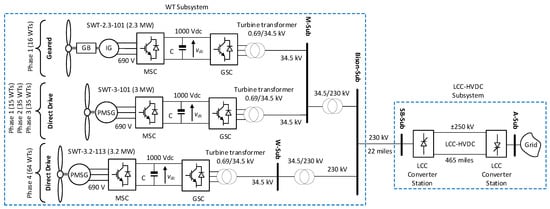
Figure 1.
Schematic of BWGS.
PMSG-based wind turbines are commonly installed in modern wind farms due to their advantages over doubly fed induction generators (DFIGs). Similarly, many HVDC projects currently in operation utilize LCC-based HVDC technology because of its lower costs, reduced station losses, and higher reliability compared to VSC-based HVDC systems [29,30]. The construction cost of LCC-HVDC systems is relatively low, and they can handle power ratings as high as 10 GW. However, they face limitations, such as commutation failures during AC faults [31]. In contrast to LCC-HVDC, VSC-HVDC systems exhibit drawbacks such as higher installation costs, lower power ratings, and increased losses resulting from their higher switching frequencies [32]. Due to the complex nature and the presence of a large number of converters and variety of control loops within the PMSG and LCC-HVDC components, the dynamic interactions become intricate and may cause SSOs. The authors in [4] utilized a state space model to analyze the oscillation characteristics in a PMSG-based wind farm integrated with LCC-HVDC, employing an eigenvalue analysis. However, the application of a state space analysis requires detailed parameters for the analysis. In the context of complex systems with multiple wind turbines, the number of state variables results in increased complexity, ultimately leading to a dimensional problem in the state space model. Therefore, in this paper, a simplified impedance-based approach is utilized to derive the impedance model of BWGS. To unveil the dynamic interactions, the overall system is divided into wind turbine (WT) subsystems and LCC-HVDC subsystems. The wind turbines are integrated into an AC collector grid through a pair of back-to-back VSCs comprising an MSC and a GSC. These converters serve to uncouple the variable-speed generator from the grid, ensuring compatibility with its fixed voltage and frequency. Wind turbines installed at BWGS operate in grid following mode, where the MSC controls the wind speed by using a field-oriented control and the GSC operates in DC voltage control. The MSC governs the wind turbine speed through field-oriented control, leveraging maximum power point tracking (MPPT) to extract the power from the wind velocity. Simultaneously, the GSC manages the active and reactive power flow to the grid while upholding a constant DC-link voltage. The control scheme utilized for both the MSC and GSC is depicted in Figure 2. Within the MSC, the MPPT system ensures optimal power extraction. The transformation from abc to d–q variables within the MSC is facilitated by considering the rotor angle position . Subsequently, the resultant error signal is fed into a proportional–integral (PI) controller that finely tunes the switching operations within the MSC to sustain this optimal power point. Conversely, within the GSC, a PLL is utilized to derive the angle . Active power regulation is governed by the d-axis current , while the q-axis current oversees the reactive power of the wind generator. Typically, the reference q-axis current is set to zero to ensure the operation of wind turbine at a unity power factor. The control of the GSC is achieved by considering the d–q rotating reference frame using the grid voltage and current as a reference. Following Park’s transformation, these measured values are converted into the d–q domain, denoted as and . The error signal undergoes processing by the controller, and subsequently, the inverse Park’s transformation converts the signals back to the abc domain, enabling the appropriate switching to control active and reactive power flow into the grid. Furthermore, an outer loop controller for the DC link voltage is employed to regulate the DC voltage . The passive components , , and are the filter resistance, inductance, and capacitance, respectively. The parameters of the wind turbine system are shown in Table 1.
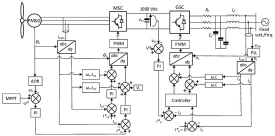
Figure 2.
Control schematic of the machine side and grid side converter (* Reference signal).

Table 1.
Parameters of the wind turbine system.
2.2. Square Butte LCC-HVDC
The Square Butte HVDC substation, as part of the BWFG system, was installed to transmit bulk power from Center, North Dakota, to Arrowhead in Minnesota and was commissioned in 1977. The Square Butte HVDC system operates as a bipolar transmission line, delivering a rated capacity of 500 MW at a bipolar voltage of KV DC with a current rating of 1000 A per pole. The system can transfer a maximum of 550 MW (1100 Amps) in bipolar operations and up to 275 MW (1100 Amps) in single-pole operations, using either metallic return or ground return in emergency situations. A simplified single-line diagram of Square Butte LCC-HVDC is shown in Figure 3, whereas the detailed parameters of the system are shown in Table 2. From the single-line diagram, it can be seen that two 11th and 13th AC harmonic filters, each rated at 39 MVAr, are symmetrically installed at each terminal. Additionally, two high-pass filters, each rated at 30 MVAr, are installed at both ends. For DC side harmonic filtering, the system also employs double-tuned DC filters, specifically targeting the 12th and 24th harmonic frequencies. The core of the system lies in its indoor, air-insulated, and air-cooled thyristor valves. These valves employ a quadruple valve design, with three quadruple valves forming a single 12-pulse converter unit. Each valve arm features a series connection of 144 thyristors, with no parallel connections. Finally, a smoothing reactor is placed on the high-voltage side of the system. This reactor is rated at 250 kV DC, 1000 A, and has an inductance of 0.06 Henry. The rectifier and inverter at the square Butte LCC-HVDC system operate under constant current control and constant extinction angle control, respectively. At the rectifier terminal, the DC current is measured, and a reference firing angle is generated, which is then compared with the phase angle of the voltage measured at the point of interconnection (POI). Conversely, at the inverter terminal, the voltage at the DC bus is measured to generate a reference firing angle, which is then compared with the phase angle of the grid voltage to generate the control signal. Figure 4 illustrates a detailed connection and control of a single-pole 12-pulse valve group comprising a rectifier station operating in DC current control mode and an invert station for DC bus voltage control. Here, denotes the reference firing angle, while represents the phase angle measured at the SB and AE subs, respectively. The detailed control scheme of the LCC-HVDC rectifier and inverter under normal operation is shown in Figure 5 [22]. Here, , and represents the measured and reference current for rectifier control, while and denotes the measured and reference voltage for inverter control.
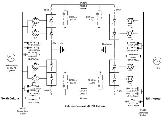
Figure 3.
Simplified single-line diagram of Square Butte LCC-HVDC.
Table 2.
Parameters of the LCC HVDC.
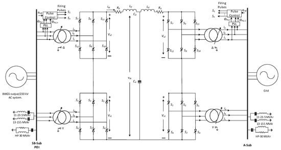
Figure 4.
Typical connection and control of a single-pole 12-pulse valve group.
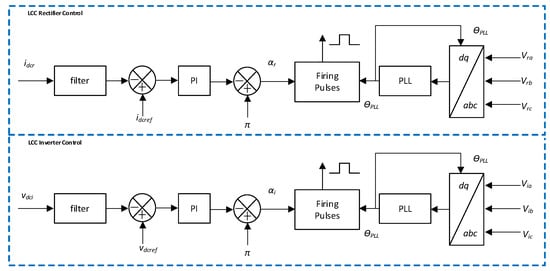
Figure 5.
Control scheme of rectifier and inverter.
To generate the control signal and initiate the switching, the reference firing angle of the rectifier () and inverter () are compared with the phase angle estimated from the AC voltage. The resultant control signal is then transmitted to the rectifier and inverter stations. In the rectifier control scheme, the measured DC current undergoes filtration before being applied to the controller. PI controllers are utilized in both control loops for regulation purposes, while a PLL is employed to obtain the electrical angle for the abc–d–q transformation. In the phase-controlled LCC, the firing angle is compared with a voltage angle reference, and thyristors are turned on when the reference signal (usually a control signal) exceeds the firing angle, which are generated by the PLL and current control loop, respectively. The firing angle () at time t represents the delay in the conduction of the thyristors after the instant the voltage crosses zero. When the reference signal surpasses this firing angle, it triggers the thyristor to conduct, allowing current to flow through the converter circuit. This control mechanism allows the converter to regulate the power flow and achieve the desired performance, such as controlling the voltage, current, or power factor in the system. Figure 6a,b show the LCC rectifier operation and pulse generation mechanism for the switching of thyristors.
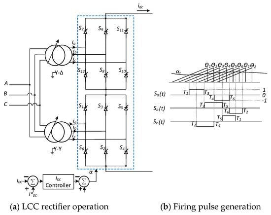
Figure 6.
LCC Rectifier operation and firing pulse generation.
3. Frequency Scan and Impedance Data Curation
Acquisition of impedance models through measurement is important in understanding complex systems. When dealing with a highly complex or black-boxed system, deriving an analytical model can be challenging and require significant simplification and assumptions, which can limit the accuracy of the resulting model. In such circumstances, two methods are mainly employed for impedance measurements: (1) frequency scanning [20,33] or harmonic injection [28], and (2) online measurement [34]. Online measurement involves the use of an additional hardware device, known as an impedance measurement unit (IMU), which injects voltage perturbations, collects the resulting voltage and current, and computes the d–q impedance. Compared to the online measurement at the initial stage, the frequency scanning method is favored for its simpler experimental design. This technique involves injecting a broad-spectrum signal into the system during normal operation. By analyzing the system’s response to this signal, a mathematical model of its small-signal impedance or admittance in d–q or the sequence domain can be extracted [35]. Frequency scanning is a valuable technique for extracting system models. It utilizes a time–domain simulation program to analyze how the system responds to a wide range of small-signal frequencies. This analysis is then numerically converted into a mathematical model through FFT to break down the system’s response and vector fitting algorithms to identify key characteristics, allowing for the creation of an accurate model. While traditional frequency scanning methods have limitations, the authors in [33] explore the use of d–q and dynamic phasor-based frequency scanning.
To perform the impedance test, a frequency scan is utilized to determine the equivalent impedance of the wind farm and LCC-HVDC system connected to the grid. Perturbations were applied at POI, and the system’s response was analyzed across a wide range of frequencies to extract the d–q impedance components. Following the scan, voltage and current signals are recorded and processed using MATLAB 2022, where FFT is employed to extract the frequency components, resulting in frequency domain impedance data. Although the existing methods to perform an impedance-based stability analysis have demonstrated strong effectiveness, errors in impedance modeling can occur, particularly due to approximation during linearization in analytical impedance modeling. In our specific case, utilizing frequency scan-based impedance modeling, errors can arise, particularly in the presence of weak or unbalanced grid conditions. These conditions can lead to inaccuracies in phase determination by the PLL. However, enhancing the PLL structure improves the impedance modeling and stability analysis. Figure 7 illustrates the key steps in the methodology for performing frequency scanning and an impedance-based stability analysis of the overall system. The system under consideration is simplified into two sub systems, the BWGS serving as the source, and the grid acting as the load. Scanning individual frequencies is time-consuming; therefore, the spectrum of the frequency and multirun component in PSCAD/EMTDC is utilized to perform repeated tasks. The simulation utilizes a time step of 20 μs and a maximum duration of 5.0 s. The perturbation is applied at POI with a perturbation voltage of 1% of the nominal voltage. Frequency scanning can be performed using either voltage or current perturbations to the system. Interestingly, both methods generally yield similar results and accuracy. In this approach, a small, perturbed voltage is introduced around the system’s operating point. The system’s response is then analyzed across a wide range of frequencies to extract the d–q impedance components, which provide valuable insights into the system’s behavior. The injected signal is a multi-sine periodic waveform superimposed on the existing sources necessary to establish the operating conditions. A multi-sine voltage perturbed signal is given by (1) and is used as a wideband signal to perturb the system [36]. The perturbed voltage signal is of a small magnitude so that the steady-state operation is not affected.
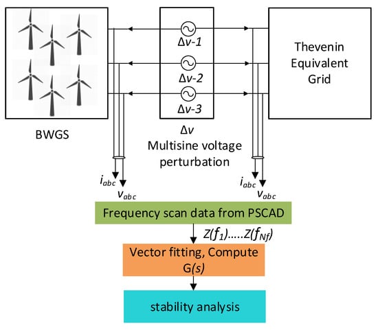
Figure 7.
Methodology used to perform the stability analysis.
In Equation (1), is the amplitude, is the frequency interval of the injected signal and is the phase shift.
Once the scan is performed, the recorded voltage and current signals are processed in MATLAB, where a FFT is used to extract the frequency components and resulting d–q impedance. , , , and are calculated as shown in (2). The resulting impedance matrix is given by (3).
In Equation (2), is the perturbation frequency.
4. Vector Fitting (VF) and LTI Modeling
The vector fitting algorithm, first introduced in [37], is a widely adopted technique for effectively approximating unknown system models using frequency response data acquired from simulations or measurements. A series of discrete terminal impedances obtained through simulations can be modeled in the Laplace domain using the VF algorithm, as detailed in the flow chart shown in Figure 8. Employing an iterative least-squares error minimization approach (4), the VF algorithm progressively refines a rational fitting function, to closely match the simulated data, . The VF algorithm leverages the pole-residue representation of transfer functions (5) in a single-input, single-output (SISO) case, and this representation aligns with the partial fraction expansion of The fitted transfer function is estimated using -iterations by minimizing the least square error and fitted transfer function is the sum of rational functions defined in (6), where real poles and residues are represented by and , while the imaginary residue and poles are given by and , and represents a real constant [38]. Equations (4)–(6) are integral to the vector fitting algorithm, which is employed to estimate the transfer function of the overall system. The simulated data and the desired approximation order are the input to the VF algorithm. In general, the higher the value of , the lower the RMS error will be, and the fitted model will be more accurate. In order to accurately capture the behavior of the measuring system, various LTI representation options were investigated. These options involved altering the order and pole location of the fitting model. The optimal LTI representation will therefore be determined by minimizing the root mean square (RMS) error while retaining the stable dynamics that are inherent in the original system.
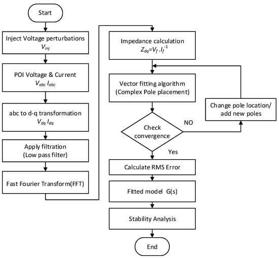
Figure 8.
Flow chart of the scheme.
Here, are the poles, is the residue corresponding to the poles, and parameter takes a non-zero value when , while is also non-zero in case .
The flow chart in Figure 8 describes the working principle of frequency scan and the VF algorithm. After performing a frequency scan and applying FFT, the resulting frequency domain impedance data are input into the vector fitting algorithm. To accurately capture the resonance peaks during the fitting process, the algorithm [37] initializes the pole locations with complex values. While the initial pole locations are arbitrarily chosen, the subsequent pole relocation step iteratively refines them until a minimum error is achieved. This iterative process converges when the least-squares error falls below a predefined threshold (), indicating a satisfactory model fit. Following the convergence check and calculation of residues, the process yields a transfer function that accurately emulates the system frequency-dependent impedance model of the system for the stability analysis.
5. Impedance-Based Stability Analysis
The impedance-based stability analysis stands out as a data-driven tool that has demonstrated efficacy in assessing the stability of wind farms connected to the grid. Various studies have explored the use of impedance-based stability analyses in conjunction with frequency scanning of power systems [38]. Using time–domain electromagnetic transient (EMT) simulations alongside frequency scanning allows for the estimation of impedance models of a power system. The system under consideration consisting of BWGS and LCC-HVDC transmission, as shown in Figure 1, is modeled in PSCAD/EMTDC, and the frequency scan is performed in the d–q domain. During the simulations, the coupling impedances were considered, with and recorded to calculate both self and coupling impedances. However, due to the relatively small magnitude of and compared to the direct and quadrature impedances, the impedance matrix is considered diagonally dominant. Therefore, only and were utilized in the stability analysis. The work presented in this paper builds upon the methodologies outlined in [39,40], where stability analyses were performed using only the diagonal impedances and . Specifically, given the complexity of a system comprising hundreds of turbines, simplifying the stability criterion by focusing on diagonal impedances helps mitigate the computational burden without compromising the overall validity of the analysis. Furthermore, while coupling impedance can indeed provide additional insights into system behavior, our analysis indicates that for the specific conditions of the BWGS, the diagonal impedances and adequately capture the primary characteristics influencing stability. The flow chart in Figure 8 shows the steps involved in performing the frequency scan and stability analysis. The parameters used in the simulation are listed in Table 1 and Table 2. To assess potential instabilities, an estimation of the transfer function the vector fitting algorithm is used to approximate the impedance data obtained from simulations, resulting in an LTI approximation model of the PMSG and LCC-HVDC system. The obtained model is employed to analyze the potential instability in the interconnected system and propose adjustments to control parameters, thereby facilitating the achievement of the desired response. Following the VF-based estimation of the transfer function, the Bode plot for both the fitted model and the simulated frequency response data are plotted. The order of the fitting function in the VF method is set to 20, a choice made based on considerations of convergence speed and fitting accuracy. Subsequently, after determining the fitting model using the VF algorithm, Bode plots illustrating the magnitude and phase are generated. To understand the dynamic behavior and stability of the PMSG-based wind farm and LCC-based HVDC, several case studies were conducted.
The Bode diagrams in Figure 9 illustrate the simulated impedance frequency response for case-1 alongside the fitting results obtained using various orders. The solid line depicts the simulated frequency response, while the dashed line represents the corresponding vector fitting approximation achieved using the VF algorithm. It is evident from the results that the fitting accuracy improves with increasing order, notably from the 8th to the 20th order. Our study demonstrates that a satisfactory approximation of the impedance response is attained with an order of 20. The RMS fitting errors for various orders are summarized in Table 3.
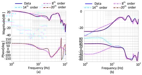
Figure 9.
Fitting results of simulated BWGS output impedance using different orders: (a) (b) .
Table 3.
Fitting errors.
5.1. Stability Analysis of BWGS
To study the resonance and operational stability of BWGS, we consider the phase difference between the grid impedance () and the output impedance of BWGS () at frequencies where their magnitude responses interact. The occurrence of resonance phenomenon is indicated when the magnitude of the impedance of BWGS and the grid overlap at a certain frequency. Therefore, at a resonance frequency, the system will demonstrate stability if and only if the phase difference between and is less than , i.e., [41]. A phase difference equal to produces an oscillatory response, and the system may be considered marginally stable. However, a phase difference greater then can lead to potential resonance of a high magnitude, causing the system to become unstable. To observe the resonance, the SCR of the grid is varied, and a stability analysis of BWGS is conducted. The stiffness of the grid at POI can be characterized by the SCR, represented as follows:
where is the short circuit capacity at the POI, i.e., the Bison-sub, as shown in Figure 1; is the total apparent power of BWGS; is the grid voltage amplitude; and are the amplitude of the rated POI voltage and current injected by the BWGS in to the grid.
Initially, the frequency scan is performed considering a strong grid with a SCR of 12. Equations (1)–(7) are used during different steps of the analysis, as shown in Figure 8. Initially, Equations (1)–(3) are used to inject the voltage perturbation and simultaneously calculate the impedance of the system. In the second stage, Equations (4)–(6) are utilized in vector fitting and transfer function estimation. Finally, Equation (7) aids in calculating the SCR and performing the stability analysis. Once the frequency scan is completed, the resulting data undergo processing as outlined in the flow chart depicted in Figure 8. Subsequently, the magnitude and phase plot for , , and are illustrated in Figure 10. The analysis reveals that the magnitude curve of the wind farm impedance and interact between 90 and 100 Hz; however, the corresponding phase difference is small, indicating the stability of the system. Conversely, the impedance curve of the wind farm ( does not interact with , indicating that the quadrature-axis component of the BWGS at a high SCR value is not contributing to the resonance. In conclusion, the phase difference between and for a robust grid remains below , affirming system stability. In addition, it can also be noticed that the wind farm impedance is capacitive before interacting with the grid impedance; therefore, a decrease in the SCR value or increases in the output power of the wind farm may cause the impedance curve of the wind farm to interact with the grid impedance curve with a higher phase difference, potentially causing instability. To analyze the stability of the interconnected system, the SCR of the grid is reduced to 5. The resulting Bode plots, as depicted in Figure 11, illustrate that as the SCR of the grid decreases, the magnitude curve of the wind farm impedance and interact between 90 and 100 Hz, with a phase difference of 110 degrees. In addition, the magnitude curve of the wind farm impedance and also interact between 80 and 90 Hz, with a phase difference of 90 degrees. However, the phase difference between and the , curves is less then , indicating that the system is stable. To further investigate the effects of grid strength on system stability, the SCR of the grid is reduced to 2, and the resulting Bode plot is shown in Figure 12. Notably, the analysis reveals that both and interact with at a frequency of 90 Hz. In this instance, there is a significant increase in the phase difference between the grid impedance and the wind farm impedance , plots, particularly on the plot, surpassing the threshold of . The surpassing of the limit indicates a strong interaction between the wind output and the grid, potentially leading to oscillatory behavior of the system. Additionally, when the phase difference between the grid impedance and the wind farm impedance exceeds 180 degrees, it can lead to resonance, voltage instability, power quality issues, and control instability, ultimately resulting in system instability.
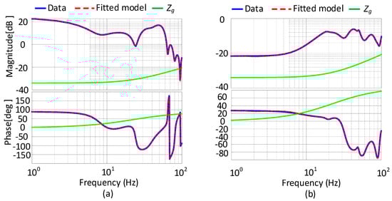
Figure 10.
Output impedance of BWGS when grid SCR = 12. (a) , (b) .
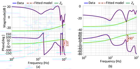
Figure 11.
Output impedance of BWGS when grid SCR = 5. (a) , (b) .
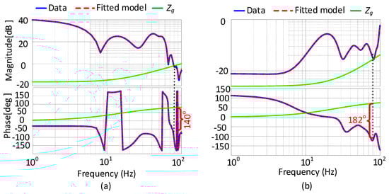
Figure 12.
Output impedance of BWGS when grid SCR = 2. (a) , (b) .
5.2. Stability Analysis of LCC-HVDC
To perform a stability analysis of the Square Butte LCC-HVDC system, the configuration depicted in Figure 3 is modeled in PSCAD/EMTDC. The methodology used in the flow chart in Figure 8 is employed to derive the impedance model of the LCC-HVDC using a frequency scan followed by the vector fitting algorithm to perform the stability analysis. Variations in the SCR and PLL bandwidth are employed to investigate the stability of the LCC-HVDC system connected to the PMSG-based wind farm. Initially, the LCC-HVDC system is connected to a strong grid with SCR = 6 at rectifier side in center (North Dakota), and the power is being transmitted through the LCC-HVDC transmission system to Arrowhead (Minnesota) under the strong grid scenario. The magnitude and phase plot for , , and are illustrated in Figure 13. The analysis reveals that the magnitude curve of the LCC-HVDC impedance and do not interact. Therefore, it can be determined that the system operates in stable mode. In the second case, the SCR of the grid is decreased to 3, and the resulting Bode plot is shown in Figure 14. The interaction between the magnitude of the grid impedance and the LCC-HVDC impedance can be observed in the plot; however, the impedance does not show any interactions with the grid impedance, indicating that does not contribute to the resonance in the system.
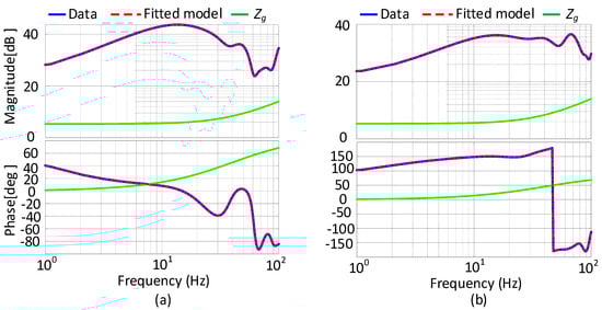
Figure 13.
Output impedance of LCC-HVDC when grid SCR = 6. (a) , (b) .
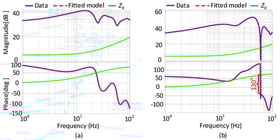
Figure 14.
Output impedance of LCC-HVDC when grid SCR = 3. (a) , (b) .
Finally, the SCR of the grid is further reduced to 2, and the resulting Bode plots are shown in Figure 15. In this scenario, both the and plots interact with the grid impedance, and the phase difference in exceeds , which can trigger instability in the system. Additionally, there are two interaction points between and the LCC-HVDC output impedance on the plot. The first occurs at 70 Hz; however, at this frequency, the phase difference is small, measuring only , indicating system stability. However, at a frequency of 90 Hz, the phase difference exceeds , indicating that the system will eventually become unstable. To delve deeper into the impact of the system parameters, we adjust the frequency bandwidth of the PLL and conduct an analysis of its influence on overall stability. Figure 16 presents the Bode plot illustrating the impedance characteristics of the LCC-HVDC system interconnected with a wind farm, depicting various PLL frequency bandwidth values. Initially, the PLL frequency bandwidth is configured at 20 Hz.
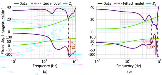
Figure 15.
Output impedance of LCC-HVDC when grid SCR = 2. (a) , (b) .
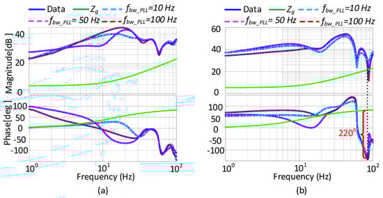
Figure 16.
Output impedance of LCC-HVDC for different frequency bandwidths of PLL. (a) , (b) .
Our analysis indicates minimal interactions between the grid impedance and the LCC-HVDC impedance, with no observable resonance contribution evident in the and impedance plots. Subsequently, we increased the PLL bandwidth to 50 Hz. Even with this adjustment, the system operates in the stable mode, showing no susceptibility to resonance. However, when we further raise the PLL bandwidth to 100 Hz, our analysis reveals a significant interaction between the grid and LCC-HVDC impedances. This interaction is marked by a phase difference exceeding 180 degrees at the point where the magnitudes of both impedances coincide. This scenario indicates a potential for resonant frequencies to emerge, presenting a destabilizing threat to the BWGS. Additionally, we observe that the impedance remains relatively constant, owing to the PLL’s regulation of q-axis voltages.
6. Conclusions
In this paper, a comprehensive impedance-based stability assessment methodology for PMSG-based wind farms connected to LCC-HVDC systems is presented. The stability of BWGS, a real-world wind farm located in North Dakota, United States, is investigated using frequency scanning techniques. The d–q impedance model of the PMSG-based wind farm and LCC-HVDC system at the BWGS is extracted. An LTI representation of the system’s dynamics is obtained through VF, followed by stability analyses conducted via Bode plot analyses. The methodology in the paper offers an approach to assess the risk of possible unstable operation of wind farms connected to HVDC systems. Specifically, the influence of the SCR of the grid and the PLL frequency bandwidth on the stability of the collector grid and LCC-HVDC system is examined. The dynamic interaction of the wind farm and LCC-HVDC with the grid is studied in detail by considering different values of SCR. The extracted d–q impedance model accurately provides information for the system stability evaluation and can be used for parameter design to avoid SSO incidents. These findings offer valuable insights for the design and verification of AC collectors and LCC-based HVDC transmission systems. The findings highlight the robustness and accuracy of frequency scanning and VF-based impedance modeling in investigating system dynamics, unstable operating conditions, and control interactions.
Author Contributions
Writing—original draft preparation, M.A.; writing—review and editing, M.A. and O.B.; conceptualization, M.A., M.O.M. and M.G.; methodology, M.A. and O.B.; software, M.A. and M.O.M.; formal analysis and investigation, M.A. and O.B.; resources, M.A. and M.G.; data curation, M.A.; supervision and project administration, O.B. All authors have read and agreed to the published version of the manuscript.
Funding
This research received no external funding.
Data Availability Statement
The data used during the study is available from the corresponding author upon reasonable request.
Conflicts of Interest
The author declares no conflict of interest.
References
- Abedin, T.; Lipu, M.S.H.; Hannan, M.A.; Ker, P.J.; Rahman, S.A.; Yaw, C.T.; Tiong, S.K.; Muttaqi, K.M. Dynamic Modeling of HVDC for Power System Stability Assessment: A Review, Issues, and Recommendations. Energies 2021, 14, 4829. [Google Scholar] [CrossRef]
- Gao, B.; Deng, P.; Wang, Y.; Yu, H.; Ren, B. Evaluation of damping of sub synchronous interaction between direct-drive wind farm and LCC-HVDC based on the damping path analysis. Int. J. Electr. Power Energy Syst. 2023, 144, 108532. [Google Scholar] [CrossRef]
- Lee, J.-S.; Lee, G.-Y.; Park, S.-S.; Kim, R.-Y. Impedance-Based Modeling and Common Bus Stability Enhancement Control Algorithm in DC Microgrid. IEEE Access 2020, 8, 211224–211234. [Google Scholar] [CrossRef]
- Zheng, L.; Ma, S. Damping Characteristic Analysis and Optimization of Wind-thermal-bundled Power Transmission by LCC-HVDC Systems. J. Mod. Power Syst. Clean Energy 2024, 12, 299–312. [Google Scholar] [CrossRef]
- Fan, L.; Miao, Z. Time-Domain Measurement-Based DQ-Frame Admittance Model Identification for Inverter-Based Resources. IEEE Trans. Power Syst. 2021, 36, 2211–2221. [Google Scholar] [CrossRef]
- Xie, X.; Zhang, C.; Liu, H.; Liu, C.; Jiang, D.; Zhou, B. Continuous-Mass-Model-Based Mechanical and Electrical Co-Simulation of SSR and Its Application to a Practical Shaft Failure Event. IEEE Trans. Power Syst. 2016, 31, 5172–5180. [Google Scholar] [CrossRef]
- Lyu, J.; Cai, X.; Amin, M.; Molinas, M. Sub-synchronous oscillation mechanism and its suppression in MMC-based HVDC connected wind farms. IET Gener. Transm. Distrib. 2018, 12, 1021–1029. [Google Scholar] [CrossRef]
- Bahrman, M.; Larsen, E.; Piwko, R.; Patel, H. Experience with HVDC—Turbine-Generator Torsional Interaction at Square Butte. IEEE Trans. Power Appar. Syst. 1980, PAS-99, 966–975. [Google Scholar] [CrossRef]
- Gao, B.; Liu, Y.; Shao, B.; Ran, H. A path analysis method to study the sub synchronous oscillation mechanism in direct-drive wind farm with VSC-HVDC system. Int. J. Electr. Power Energy Syst. 2022, 142, 108328. [Google Scholar] [CrossRef]
- Chao, W.; Deng, C.; Huang, J.; Dai, L.; Min, Y.; Cheng, Y.; Wang, Y.; Liao, J. A Sub-Synchronous Oscillation Suppression Strategy Based on Active Disturbance Rejection Control for Renewable Energy Integration System via MMC-HVDC. Electronics 2023, 12, 288. [Google Scholar] [CrossRef]
- Cheng, Y.; Fan, L.; Rose, J.; Huang, S.-H.; Schmall, J.; Wang, X.; Xie, X.; Shair, J.; Ramamurthy, J.R.; Modi, N.; et al. Real-World Sub synchronous Oscillation Events in Power Grids with High Penetrations of Inverter-Based Resources. IEEE Trans. Power Syst. 2023, 38, 316–330. [Google Scholar] [CrossRef]
- Arshad, M.; Beik, O.; Pallapati, R.; Hoberg, S. Overview and Impedance-Based Stability Analyses of Bison Wind Farm: A PRACTICAL EXAMPLE. IEEE Ind. Appl. Mag. 2024, 2–15. [Google Scholar] [CrossRef]
- Liu, B.; Li, Z.; Zhang, X.; Dong, X.; Liu, X. Impedance-Based Analysis of Control Interactions in Weak-Grid-Tied PMSG Wind Turbines. IEEE J. Emerg. Sel. Top. Circuits Syst. 2020, 11, 90–98. [Google Scholar] [CrossRef]
- Guo, B.; Zhang, X.; Ma, H.; Yang, Y.; Wang, X.; Tian, Q.; Jin, S. A Series Impedance Reshaping Control Method Considering PLL Dynamics for Grid-Connected Inverters Under Weak Grid Conditions. IEEE Trans. Ind. Electron. 2024, 71, 4896–4910. [Google Scholar] [CrossRef]
- Amin, M.; Molinas, M. Understanding the Origin of Oscillatory Phenomena Observed between Wind Farms and HVDC Systems. IEEE J. Emerg. Sel. Top. Power Electron. 2017, 5, 378–392. [Google Scholar] [CrossRef]
- Zhu, Y.; Gu, Y.; Li, Y.; Green, T. Participation Analysis in Impedance Models: The Grey-Box Approach for Power System Stability. IEEE Trans. Power Syst. 2022, 37, 343–353. [Google Scholar] [CrossRef]
- Wang, Z.; Bao, L.; Fan, L.; Miao, Z.; Shah, S. From Event Data to Wind Power Plant DQ Admittance and Stability Risk Assessment. IEEE Trans. Power Syst. 2022, 37, 4400–4408. [Google Scholar] [CrossRef]
- Liu, B.; Li, Z.; Dong, X.; Yu, S.S.; Chen, X.; Oo, A.M.T.; Lian, X.; Shan, Z.; Liu, X. Impedance Modeling and Controllers Shaping Effect Analysis of PMSG Wind Turbines. IEEE J. Emerg. Sel. Top. Power Electron. 2020, 9, 1465–1478. [Google Scholar] [CrossRef]
- Gholamian, M.; Beik, O. Coordinate Control of Wind Turbines in a Medium Voltage DC Grid. IEEE Trans. Ind. Appl. 2023, 59, 6480–6488. [Google Scholar] [CrossRef]
- Jiang, X.; Gole, A. A frequency scanning method for the identification of harmonic instabilities in HVDC systems. IEEE Trans. Power Deliv. 1995, 10, 1875–1881. [Google Scholar] [CrossRef]
- Badrzadeh, B.; Sahni, M.; Zhou, Y.; Muthumuni, D.; Gole, A. General methodology for analysis of sub-synchronous interaction. IEEE Trans. Power Syst. 2013, 28, 1858–1869. [Google Scholar] [CrossRef]
- Liu, Y.; Zhou, X.; Chen, Q.; Yin, H.; Hong, L.; Tian, H.; Chen, Y.; Li, S. Harmonic State Space Based Impedance Modeling and Virtual Impedance Based Stability Enhancement Control for LCC-HVDC Systems. J. Mod. Power Syst. Clean Energy 2024, 12, 287–298. [Google Scholar] [CrossRef]
- Zhou, W.; Mohammed, N.; Bahrani, B. Comprehensive Modeling, Analysis, and Comparison of State-Space and Admittance Models of PLL-Based Grid-Following Inverters Considering Different Outer Control Modes. IEEE Access 2022, 10, 30109–30146. [Google Scholar] [CrossRef]
- Bakhshizadeh, M.K.; Blaabjerg, F.; Hjerrild, J.; Kocewiak, L.; Bak, C.L. Improving the Impedance-Based Stability Criterion by Using the Vector Fitting Method. IEEE Trans. Energy Convers. 2018, 33, 1739–1747. [Google Scholar] [CrossRef]
- Kontis, E.O.; Papadopoulos, T.A.; Chrysochos, A.I.; Papagiannis, G.K. Measurement-Based Dynamic Load Modeling Using the Vector Fitting Technique. IEEE Trans. Power Syst. 2018, 33, 338–351. [Google Scholar] [CrossRef]
- Chen, C.; Gong, L.; Qian, W.; Zhang, W.; Wu, T.; Li, X. Study on Wideband Harmonic Instability of Wind Farm Based on the Vector Fitting Method. In Proceedings of the 2023 International Seminar on Computer Science and Engineering Technology (SCSET), New York, NY, USA, 29–30 April 2023; pp. 737–741. [Google Scholar]
- Xue, T.; Lyu, J.; Wang, H.; Cai, X. A Complete Impedance Model of a PMSG-Based Wind Energy Conversion System and Its Effect On the Stability Analysis of MMC-HVDC Connected Offshore Wind Farms. IEEE Trans. Energy Convers. 2021, 36, 3449–3461. [Google Scholar] [CrossRef]
- Salehi, F.; Matsuo, I.B.M.; Brahman, A.; Tabrizi, M.A.; Lee, W.J. Sub-Synchronous Control Interaction Detection: A Real-Time Application. IEEE Trans. Power Deliv. 2019, 35, 106–116. [Google Scholar] [CrossRef]
- Feng, J.; Liu, Z.; Li, K.; Li, B.; Li, J.; Li, L. A fast and high-accurate commutation failure identification method for LCC-HVDC system. In Proceedings of the IEEE 6th Conference on Energy Internet and Energy System Integration, Chengdu, China, 11–13 November 2022; pp. 763–767. [Google Scholar]
- Khazaei, J.; Idowu, P.; Asrari, A.; Shafaye, A.; Piyasinghe, L. Review of HVDC control in weak AC grids. Electr. Power Syst. Res. 2018, 162, 194–206. [Google Scholar] [CrossRef]
- Guo, C.; Liu, W.; Zhao, C.; Iravani, R. A Frequency-Based Synchronization Approach for the VSC-HVDC Station Connected to a Weak AC Grid. IEEE Trans. Power Deliv. 2017, 32, 1460–1470. [Google Scholar] [CrossRef]
- Xiao, H.; Sun, K.; Pan, J.; Liu, Y. Operation and control of hybrid HVDC system with LCC and full-bridge MMC connected in parallel. IET Gener. Transm. Distrib. 2020, 14, 1344–1352. [Google Scholar] [CrossRef]
- Das, M.K.; Kulkarni, A.M.; Darji, P.B. Comparison of DQ and Dynamic Phasor based frequency scanning analysis of grid-connected Power Electronic Systems. In Proceedings of the 2016 Power Systems Computation Conference (PSCC), Genoa, Italy, 20–24 June 2016. [Google Scholar]
- Jaksic, M.; Shen, Z.; Cvetković, I.; Boroyevich, D.; Burgos, R.; DiMarino, C.; Chen, F. Medium-Voltage Impedance Measurement Unit for Assessing the System Stability of Electric Ships. IEEE Trans. Energy Convers. 2017, 32, 829–841. [Google Scholar] [CrossRef]
- Dey, K.; Das, M.K.; Kulkarni, A. Comparison of dynamic phasor, discrete-time and frequency scanning based SSR models of a TCSC. Electr. Power Syst. Res. 2021, 196, 107237. [Google Scholar] [CrossRef]
- Das, M.K.; Kulkarni, A.M. Dynamic phasor based frequency scanning for grid-connected power electronic systems. Sadhana 2017, 42, 1717–1740. [Google Scholar] [CrossRef]
- Triverio, P. Vector Fitting. In Handbook on Model Order Reduction; Benner, P., Grivet-Talocia, S., Quarteroni, A., Rozza, G., Schilders, W.H.A., Silveira, L.M., Eds.; De Gruyter: Berlin, Germany, 2021; pp. 275–310. [Google Scholar]
- Jacobs, K.; Seyedi, Y.; Meng, L.; Karaagac, U.; Mahseredjian, J. A comparative study on frequency scanning techniques for stability assessment in power systems incorporating wind parks. Electr. Power Syst. Res. 2023, 220, 109311. [Google Scholar] [CrossRef]
- Aapro, A.; Messo, T.; Roinila, T.; Suntio, T. Effect of Active Damping on Output Impedance of Three-Phase Grid-Connected Converter. IEEE Trans. Ind. Electron. 2017, 64, 7532–7541. [Google Scholar] [CrossRef]
- Messo, T.; Luhtala, R.; Roinila, T.; Yang, D.; Wang, X.; Blaabjerg, F. Real-time impedance-based stability assessment of grid converter interactions. In Proceedings of the 2017 IEEE 18th Workshop on Control and Modeling for Power Electronics (COMPEL), Stanford, CA, USA, 9–12 July 2017. [Google Scholar]
- Wang, X.; Harnefors, L.; Blaabjerg, F. Unified Impedance Model of Grid-Connected Voltage-Source Converters. IEEE Trans. Power Electron. 2017, 33, 1775–1787. [Google Scholar] [CrossRef]
Disclaimer/Publisher’s Note: The statements, opinions and data contained in all publications are solely those of the individual author(s) and contributor(s) and not of MDPI and/or the editor(s). MDPI and/or the editor(s) disclaim responsibility for any injury to people or property resulting from any ideas, methods, instructions or products referred to in the content. |
© 2024 by the authors. Licensee MDPI, Basel, Switzerland. This article is an open access article distributed under the terms and conditions of the Creative Commons Attribution (CC BY) license (https://creativecommons.org/licenses/by/4.0/).