Hardware Architecture for Realtime HEVC Intra Prediction

Abstract

Researchers have, in recent times, achieved excellent compression efficiency by implementing a more complicated compression algorithm due to the rapid development of video compression. As a result, the next model of video compression, High-Efficiency Video Coding (HEVC), provides high-quality video output while requiring less bandwidth. However, implementing the intra-prediction technique in HEVC requires significant processing complexity. This research provides a completely pipelined hardware architecture solution capable of real-time compression to minimize computing complexity. All prediction unit sizes of $4\times 4$, $8\times 8$, $16\times 16$, and $32\times 32$, and all planar, angular, and DC modes are supported by the proposed solution. The synthesis results mapped to Xilinx Virtex 7 reveal that our solution can do real-time output with 210 frames per second (FPS) at $1920\times 1080$ resolution, called Full High Definition (FHD), or 52 FPS at $3840\times 2160$ resolution, called 4K, while operating at 232 Mhz maximum frequency.

1. Introduction

High-Efficiency Video Coding (H265/HEVC) is the next generation of Advanced Video Coding (H.264/AVC) compression technology, aimed at improving compression efficiency. Compared to earlier standards, H265/HEVC saves twice as much bandwidth. The desire for streaming digital video or video storing services is unavoidable as the Internet grows. H265/HEVC helps boost speed and capacity with its highly efficient coding efficiency. Moreover, H265/HEVC also outperforms high-resolution videos (4K, 8K).

Most video coding standards use intra-prediction to eliminate spatial redundancies by generating a predicted block based on nearby pixels. In H265/HEVC, the intra-prediction unit has been updated to achieve efficient coding; intra-prediction now has 35 prediction modes, nine more than H.264/AVC currently provides, and supports prediction unit (PU) sizes ranging from $4\times 4$ to $32\times 32$ (sample × sample) in comparison to the largest PU size of $16\times 16$ in H.264/AVC. H265/HEVC offers more complex intra-prediction, which has a substantial impact on coding efficiency because of the enormous computational complexity.

Intra-prediction consumes significant processing time, motivating researchers to employ various strategies to reduce algorithm complexity. Nevertheless, the output FPS of software solutions cannot meet the daily needs of the majority of consumers. Currently, streaming high-quality video in real time is common, yet, encoding these videos at high FPS is difficult with the present software solutions. As a result, we can bypass software constraints by employing hardware acceleration.

Many researchers investigated implementing the intra-prediction algorithm on hardware to achieve higher output framerates and more energy efficiency than the software version. Using the data reuse strategy for decreasing the number of computations, the proposed [1] solution helps to reduce 80% of the computation time to reach a framerate of 30 FPS for the FHD resolution. Nevertheless, it only supports PU sizes of $4\times 4$ and $8\times 8$. Therefore, the authors deploy a completely pipelined solution constructed on the Field Programmable Gate Arrays (FPGA) in the architecture [2], which supports all intra-prediction modes with all PU sizes to reach the framerate at 24 FPS for the 4K resolution.

Hasan Azgin and their colleagues proposed a Computation and Energy Reduction Method for HEVC Intra Prediction [3] in 2017. It was demonstrated that using 24.63% less energy than the original H.265/HEVC intra-prediction equation, 40 FPS can be produced for the FHD resolution at 166MHz. In 2018, [4] developed an effective FPGA implementation for the approximate intra-prediction algorithm using digital signal processing (DSP) blocks instead of adders and shifters. This design can handle 55 FPS for the FHD resolution while consuming less energy. These proposals aim to reduce computational complexity while increasing energy efficiency. However, with the continued demand for high-quality streaming video, the ability to read-time encode at the 4K resolution and high FPS is necessary.

The contributions of this paper are as follows:

(1)

We propose a completely pipelined architecture for the intra-prediction module. By implementing DC, Planer, and Angular processing units in parallel, we effectively minimize execution time to increase the throughput. The predicted samples are generated for all PU sizes in one single clock cycle.

(2)

A flexible partitioning of cell predictions was introduced for the angular prediction modes, which enhances parallelism up to 16 PUs with sizes of $4\times 4$ or $16\times 16$ each time. Our solutions provide a processing speed of 210 FPS for the FHD resolution and 52 FPS for the 4K resolution and support all prediction modes and PU sizes.

The rest of the paper is organized as follows. Section 2 explains the H.265/HEVC coding structure and intra-prediction algorithm. Section 3 explains the proposed hardware architecture for intra-prediction. Next, Section 4 and Section 5 show the functional verification and synthesis results of the proposed design. Finally, Section 6 states our conclusions.

2. Intra Coding in H.265/HEVC

2.1. Overview of H.265/HEVC Structure

An image can be divided into coding tree units (CTU) in the H.265/HEVC coding standard. Compared to the previous H.264/AVC standard, CTU is the core of the coding layer. CTUs are L × L in size, with L being 64, 32, or 16; the greatest CTU size is $64\times 64$, which is greater than a macroblock ($16\times 16$ of luma samples). H.265/HEVC can improve the previous standard’s coding efficiency by adopting a larger CTU size. H.265/HEVC employs a quad-tree partitioning structure, as illustrated in Figure 1, in which the largest coding unit (LCU) can be recursively split into four smaller coding units (CU) [5].

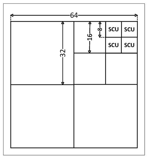
Figure 1. Demonstration of CU partitioning, where SCU is the smallest CU.

As shown in Figure 2 [6], each CU has a PU and TU (Transform Unit). The PU determines whether to use intra-picture or inter-picture prediction to reduce spatial or temporal redundancy; after obtaining the prediction residual, it is processed by the Transform Unit, which then applies entropy coding to generate the output bitstream.

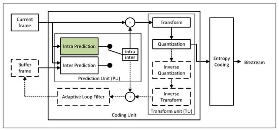
Figure 2. H.265/HEVC coding unit structure.

Intra-prediction is used in H.265/HEVC to eliminate spatial redundancy; it generates predicted samples for the PU of the CU using already coded pixels and adjoining PUs as input references. The intra-prediction algorithm supports PU sizes of $4\times 4$, $8\times 8$, $16\times 16$, and $32\times 32$, with Planar, DC, and Angular prediction modes totaling 35, as shown in Table 1.

Table 1. Intra mode number and its associated names.

Intra Prediction Mode Number	Mode Names
0	Planar
1	DC
[2, 34]	Angular

2.2. H.265/HEVC Sample Substitution and Filter

As shown in Figure 3, H.265/HEVC employs a reference sample substitution process that enables the production of predicted samples without the full availability of reference samples, where an unknown reference can be substituted by the value of its nearest reference.

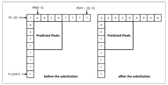
Figure 3. Illustration of sample substitution process for prediction block $4\times 4$.

Following sample substitution, input references will be conditionally filtered to avoid the appearance of undesirable directional edges on predicted samples. When the filter is applied, the three-tap filter is used as the default, and the output-filtered references are derived using the equations:

$$P[-1][-1]=\frac{P[-1]\left[0\right]+2\times P[-1][-1]+P\left[0\right][-1]+2}{4}$$

(1)

$$P[-1]\left[y\right]=\frac{P[-1][y+1]+2\times P[-1]\left[y\right]+P[-1][y-1]+2}{4}$$

(2)

$$P\left[x\right][-1]=\frac{P[x-1][-1]+2\times P\left[x\right][-1]+P[x-1][-1]+2}{4}$$

(3)

where x = [0:$2N-2$] and y = [0:$2N-2$], N is the size of predicted block.

2.3. H.265/HEVC Angular Prediction

H.265/HEVC [7] provides 33 different prediction directions in angular prediction modes, compared to only 8 in H.264/AVC [8]. Additional prediction directions allow H.265/HEVC to achieve more efficient coding with two main prediction directions: horizontal modes (modes 2–17) and vertical modes (the rest).

To perform prediction, we select positive references. The selection is followed by Equations (4) and (5):

$$R\left[x\right]=p[-1+x][-1](x\ge 0;mode\ge 18)$$

(4)

$$R\left[x\right]=p[-1][-1+x](x\ge 0;mode<18)$$

(5)

$$R\left[x\right]=p[-1][-1+((x\times B+128)>>8\left)\right](mode\ge 18)$$

(6)

$$R\left[x\right]=p[-1+((x\times B+128)>>8\left)\right][-1](mode<18)$$

(7)

For negative references, the A parameter is used for the selected mode, as shown in Table 2. If A is negative, indicating that both top and left references are required, the R needs to be extended with index $x<0$ by Equations (6) and (7). When input reference samples (R) are available, we can generate the predicted samples using the following equations:

$$R\left[x\right]\left[y\right]=\frac{\left(\right(32-f)\times R[y+i+1]+f\times R[y+i+2]+16)}{32}$$

(8)

$$R\left[x\right]\left[y\right]=\frac{\left(\right(32-f)\times R[x+i+1]+f\times R[x+i+2]+16)}{32}$$

(9)

$$i=\left(\right(y+1)\times A)>>5(mode\ge 18)$$

(10)

$$i=\left(\right(x+1)\times A)>>5(mode<18)$$

(11)

$$f=\left(\right(y+1)\times A)\&31(mode\ge 18)$$

(12)

$$f=\left(\right(x+1)\times A)\&31(mode<18)$$

(13)

Table 2. Angular A and B parameters lock-up table.

Horizontal modes	mode	2	3	4	5	6	7	8	9
	A	32	26	21	17	13	9	5	2
	mode	10	11	12	13	14	15	16	17
	A	0	−2	−5	−9	−13	−17	−21	−26
Vertical modes	mode	18	19	20	21	22	23	24	25
	A	−32	−26	−21	−17	−13	−9	−5	−2
	mode	26	27	27	29	30	31	32	33
	A	0	2	5	9	13	17	21	26
	A	−32	−26	−21	−17	−13	−9	−5	−2
	B	−256	−315	−390	−482	−630	−910	−1638	−4096

Equation (8) is used for vertical modes ($mode\ge 18$), and Equation (9) is for horizontal modes where $mode<18$, where the ranges of $xandy$ depend on the size of the prediction unit.

Discontinuities in the output result may occur during the generation of the predicted samples. These discontinuities can be removed using a boundary filter is used to smooth the predicted boundary values by replacing them with the reference samples; this step is optional for angular modes 10 and 26:

$$B_{10}\left[x\right]=CLIP(b_{10}\left[x\right]+\frac{re{f}_{top}\left[0\right]-re{f}_{top}[x+1]}{2})$$

(14)

$$B_{26}\left[x\right]=CLIP(b_{26}\left[x\right]+\frac{re{f}_{left}\left[0\right]-re{f}_{left}[x+1]}{2})$$

(15)

where $B_{10}$ is the mode 10 boundary after the filter and $B_{10}$ is the original boundary value, $re{f}_{top}$ and $re{f}_{left}$ are the top and left reference samples. In the case of an 8-bit pixel depth, the CLIP function takes the place of maintaining the predicted samples in the range $[0,255]$.

2.4. H.265/HEVC Planar Prediction

Although the angular mode delivers a decent prediction when a prediction block contains edges, it may provide some noticeable discontinuities in the results. Therefore, the following equations are employed in H.265/HEVC planar prediction to generate smooth predicted samples with no discontinuities:

$$P\left[x\right]\left[y\right]=(hor\left[x\right]\left[y\right]+ver\left[x\right]\left[y\right]+N)>>({log}_{2}N+1)$$

(16)

$$hor\left[x\right]\left[y\right]=(N-1-x)\times p[-1]\left[y\right]+(x+1)\times p\left[N\right][-1]$$

(17)

$$ver\left[x\right]\left[y\right]=(N-1-y)\times p\left[x\right][-1]+(y+1)\times p[-1]\left[N\right]$$

(18)

where P has planar predicted samples, N is the size of the prediction block, and p is references samples.

2.5. H.265/HEVC DC Prediction

DC prediction contributes to creating an absolutely smooth prediction block with no edges on the predicted output. The DC Prediction predicted samples are equal dcVal, which is derived by taking the average value of all left and top reference samples:

$$dcVal=(\sum _{x=0}^{N-1}p\left[x\right][-1]+\sum _{y=0}^{N-1}p[-1]\left[y\right]+N)>>(lo{g}_2\left(N\right)+1)$$

(19)

where N is the size of the PU, x,y = 0 …$N-1$ to determine the position of the predicted sample.

Similar to angular prediction, to avoid discontinuities, a three-tap filter is applied to replace the value of $p\left[0\right]\left[0\right]$, and a two-tap filter is applied for all predicted samples $p\left[x\right]\left[0\right]$ and $p\left[0\right]\left[y\right]$ where x = y = 1 … $N-1$:

$$p\left[0\right]\left[0\right]=\left(p\right[-1\left]\right[0]+2\times dcVal+p[0\left]\right[-1\left]\right)>>2$$

(20)

$$p\left[x\right]\left[0\right]=\left(p\right[x\left]\right[-1]+3\times dcVal+2)>>2$$

(21)

$$p\left[0\right]\left[y\right]=\left(p\right[-1\left]\right[y]+3\times dcVal+2)>>2$$

(22)

2.6. Best Mode Decision

As explained in earlier sections, H.265/HEVC has introduced a series of new prediction modes that enhance the old prediction modes of H.264/AVC to eliminate duplications in prediction and improve compression efficiency and the efficient processing of PU with complicated structures. First, the mode selection runs all 35 modes for each PU before deciding on the optimum mode to use in that PU block.

Next, the RMD (Rough Mode Decision) and RDO (Rate Distortion Optimization) are processed. The RMD process can be regarded as a pre-processing phase that minimizes the complexity of RDO by lowering the number of modes to be predicted from 35 to less and putting them in a list. Then, the modes in the list are evaluated by RDO to discover the most optimal mode for prediction.

During RMD execution, the encoder calculates the cost function for each PU using the Lagrangian cost function:

$$C{F}_{RMD}=SAD+\lambda \times R_{mode}$$

(23)

where $C{F}_{RMD}$ is the total cost required to encode a PU, and SAD (Sum of Absolute Transform Difference) is the total difference between the original and predicted PU blocks. $\lambda$ is the Lagrangian coefficient, and $R_{mode}$ is the bit rate needed to encrypt that PU block.

For RMD implementation, the decoder reduces the number of modes to perform from 35 modes to three modes (PU $64\times 64$, $32\times 32$, $16\times 16$) and eight modes (PU $8\times 8$ and $4\times 4$), with the lowest costing ones, after being calculated, added to the list of candidates. In addition, since the upper and left-adjacent PUs are related to the current PU, and these blocks have been encrypted, and the Intra mode of these blocks is also added to the list of candidates. These modes are called MPM (Most probable mode).

After completing the RMD step and adding MPM, the list of optimal modes is a total of 11 or 6 modes depending on the size of the PU. In the last step, the RDO process is performed to continue to calculate the costs of these modes and choose the lowest cost mode to apply to that PU using the following equation:

$$C{F}_{RDO}=SSE+\lambda \times R_{mode}$$

(24)

Similar to the calculation of RMD, $C{F}_{RDO}$ is the RDO cost of each PU, $\lambda$ is the Lagrangian coefficient, and $R_{mode}$ is the bit rate required to encrypt that PU block. SSE is the sum of the squared error between the current and predicted PU blocks. After the calculation is completed, the processor chooses the mode with the lowest RDO cost as the mode of execution for the current PU. This process is shown in Figure 4.

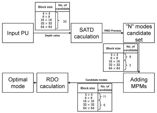
Figure 4. Process of best mode decision [9].

3. Hardware Implementation of H.265/HEVC Intra-Prediction

The proposed hardware architecture supports all intra-prediction modes, and all PU block sizes ($32\times 32$, $16\times 16$, $8\times 8$, $4\times 4$). According to Figure 5, the input reference samples are conditionally filtered and divided into three main datapaths for DC, planar, and angular prediction modules, as shown in Table 1, and the output predicted samples are fed to the SAD (Sum of Absolute Difference) module to calculate the cost for each prediction mode.

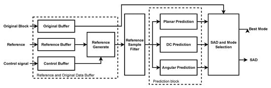
Figure 5. The proposed hardware architecture for H.265/HEVC intra prediction.

3.1. Reference Sample Filtering

In the Reference Samples Filtering stage, a three-tap filter is applied according to Equations (1)–(3); Figure 6 depicts the hardware implementation of the three-tap filter. It has a pipeline behavior and requires three adders and two shifters.

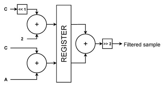
Figure 6. Implementation of a TREE-TAP FILTER.

We used a tree-tap filtering cell for each reference sample and a multiplexer to select the output-filtered references based on the size of the prediction block to filter all of the input reference samples. The configuration of three-tap filtering cells is depicted in Figure 7. Depending on the size of the prediction block, a varied number of filtering cells is triggered to generate the output. All filtering cells are activated in the $32\times 32$ block; however, only cells 0 to 8 are activated in the $4\times 4$ block. It enables the Reference Samples Filter module to process reference samples of any size without duplicating hardware resources.

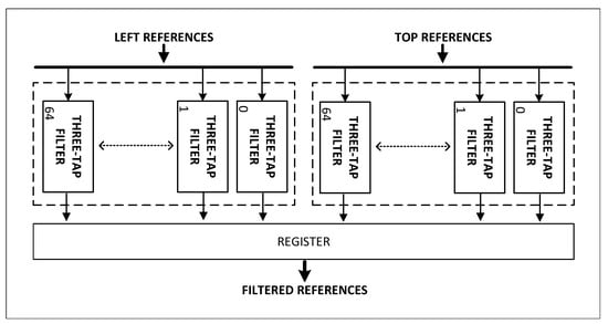
Figure 7. Hardware architecture of Reference Samples Filter module.

3.2. Angular Prediction

The angular prediction Equations (8) and (9) require reference samples and i, f values for each prediction; before delivering the predicted samples, they can be flipped or post-filtered if necessary. Figure 8 depicts our proposed hardware architecture for the Angular prediction module.

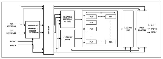
Figure 8. The proposed hardware architecture for H.265/HEVC intra Angular mode.

The top and left references are chosen in our architecture to generate main and side reference samples for the next stage. The “REFERENCE SELECT” module processes the selection using multiplexers, as shown in Figure 9.

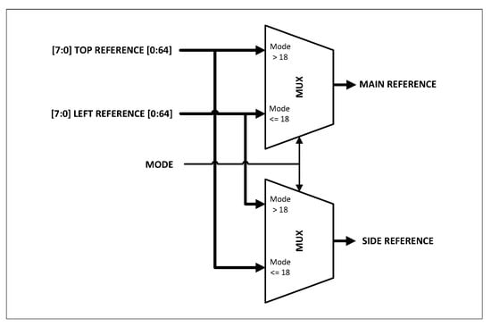
Figure 9. The method to select main and side references.

The “NEGATIVE REFERENCE EXTEND” module processes the main and side references to generate the reference with the required negative index reference samples for prediction equations later. We have already calculated i and f for each mode and kept these values in memory as a look-up table to reduce the effort of finding i and f.

To implement Equations (8) and (9) without employing a multiplier, we use the PEA [2] (Processing Element for Angular) concept. Equation (9) can be rearranged as follows:

$$R\left[x\right]\left[y\right]=\left(not\right(f)\times R[x+i+1]+f\times R[x+i+2]+16)>>5$$

(25)

As shown in Figure 10, a group of five 2to1 multiplexers and six adders is employed, and a three-stage pipeline is used to reduce propagation time and increase throughput.

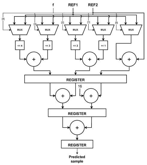
Figure 10. The structure of Processing Element for Angular (PEA) [2].

Another technique to implement Equations (8) and (9) in FPGA is to use direct multiplication operations offered by the DSP block, as shown in Figure 11. The DSP blocks are particularly efficient regarding power consumption and may be customized. Moreover, they work well with binary multipliers and accumulators. Therefore, Equation (9) should be modified using the DSP as follows:

$$R\left[x\right]\left[y\right]=(f\times (re{f}_1-re{f}_2)+((32\times re{f}_1)+16))<<5$$

(26)

$$re{f}_1=R[x+i+1]$$

(27)

$$re{f}_2=R[x+i+2]$$

(28)

$$(32\times re{f}_1)+16=(re{f}_1<<5)|16$$

(29)

Then, Equation (26) matches to the custom implementation $P=B\times (A+D)+C$ of DSP48 slice, where:

$$B=f$$

(30)

$$A=re{f}_1$$

(31)

$$D=-re{f}_2$$

(32)

$$C=(re{f}_1<<5)|16$$

(33)

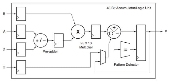
Figure 11. Basic structure of DSP48E1 Slice [10].

The biggest PU size $32\times 32$ needs 1024 PEA units to predict 1024 samples for one mode in the angular prediction architecture. The PU size $8\times 8$ needs 64 PEA units to predict 64 samples for one mode. Thus, we split those 1024 PEA units into 16 groups (64 PEA units/group), then each group is used to predict 64 samples for one mode. Therefore, 16 modes can be predicted in parallel. The parallelism for PU size $4\times 4$ is achieved in the same manner. Using flexible PEAs, we can obtain a maximum throughput of 1024 predicted samples per clock cycle. The predicted block will be flipped at the “SAMPLES FLIP” module in the case of horizontal modes. The flip process is depicted in Figure 12.

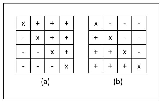
Figure 12. Illustration of the input/output of “FLIP” module for prediction block of $4\times 4$ where: (a) input predicted block, (b) flipped block output.

For modes 10 and 26, if the control signal $filter\_boundary=true$, then post-processing is required. The post-processing process applies Equations (14) and (15) to filter discontinuities in the predicted block boundary.

3.3. Planar Prediction

Module Planar prediction in Intra Prediction helps solve the image’s areas with countering and blockiness inside a PU block. Similar to Angular Prediction, we also transfer multiplications in Equations (17) and (18) into the adders and shifters module to reduce the complexity of multiplications. For example, in the case of PU size is $8\times 8$, with $N=width=8$, Equations (17) and (18) are as follows:

$$p_h\left[x\right]\left[y\right]=(7-x)\times p[-1]\left[y\right]+(x+1)\times p\left[8\right][-1]$$

(34)

$$p_v\left[x\right]\left[y\right]=(7-y)\times p\left[x\right][-1]+(y+1)\times p[-1]\left[8\right]$$

(35)

In the case of $x=1$ and $y=3$, then the formula $p_h\left[1\right]\left[3\right]$ is:

$$p_h\left[1\right]\left[3\right]=6\times p[-1]\left[3\right]+2\times p\left[8\right][-1]$$

(36)

$$p_v\left[1\right]\left[3\right]=4\times p\left[1\right][-1]+4\times p[-1]\left[8\right]$$

(37)

Two multiplications in (36) and (37) can be transformed into the shifter and adder modules according to the following formula:

$$p_h\left[1\right]\left[2\right]=(p[-1]\left[2\right]>>2+p[-1]\left[2\right]>>1)+(p\left[8\right][-1]>>1)$$

(38)

$$p_v\left[1\right]\left[2\right]=(p\left[1\right][-1]>>2)+(p[-1]\left[8\right]>>2)$$

(39)

Compared to employing multipliers, this transformation uses a set of shifters and adders instead of multipliers, as shown in Figure 13, which reduces the resources required to calculate the values of $p_h$ and $p_v$.

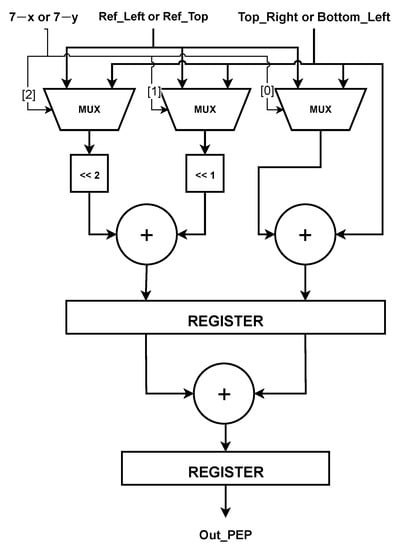
Figure 13. The structure of Processing Element for Planar (PEP) [2].

The module’s input is determined by whether the calculated value is $p_h$ or $p_v$. If $p_h$ is the calculating value, the input value will be $(7-x)$, left reference samples, $p[-1]\left[N\right]$ value, and reversed. These two numbers will be calculated in parallel simultaneously to increase throughput.

Figure 13 depicts a module with a two-stage pipeline to calculate in the situation of a PU size $8\times 8$, in which the values of $(7-x)$ and $(7-y)$ shift from 0 (0 0 0) to 7 (1 1 1). As a result, it requires three bits to cover all cases, with these bits simultaneously acting as the input for three corresponding multiplexers. If $select=1$, the selected values will be identical to the value of the reference sample. If $select=0$, the input values will be either Top_Right ($p\left[8\right][-1]$) or Bottom_Left ($p[-1]\left[8\right]$) depending on which value needs to be calculated. Then, these values are combined to produce the calculation-required value of $p_h$ and $p_v$ [2].

The number of multiplexers and shifters used to decode the relevant bits varies depending on the PU size. A maximum of five multiplexer sets for PU $32\times 32$ and a minimum of 2 multiplexer sets for PU $4\times 4$.

These modules are used as the sub-modules to operate Equation (16), thus creating predicted samples for 8 × 8 size module, as shown in Figure 14. The same method is used for $4\times 4$, $16\times 16$, and $32\times 32$ PU sizes.

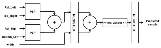
Figure 14. Hardware architecture of Planar sample prediction.

The Planar Prediction module’s output is the predicted sample values at the location that has to be predicted after using the Planar Prediction algorithm. Then, depending on the processing PU size, these values are chosen by employing a multiplexer. The selection signal input of this multiplexer is controlled by the value of $log2\left(N\right)$, as shown in Figure 15.

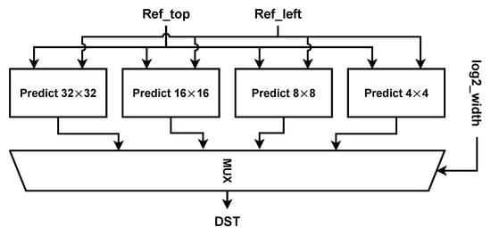
Figure 15. Hardware architecture planar prediction.

3.4. DC Prediction

The architecture of the module DC prediction is relatively straightforward because the outcome of DC Prediction is simply a calculated dcVal value based on the sum of left and top reference samples, which are then attached to every single output sample $p\left[x\right]\left[y\right]$ location inside the PU block.

In this module, the values of the top and left reference samples are sequentially passed by the add module to be added. In the case of PU size $32\times 32$, we employ a pipelined adder tree with 63 adder stages for adding at this step. It takes six clock cycles to add all of the left and top references.

The values of $p\left[0\right]\left[0\right]$, $p\left[x\right]\left[0\right]$, and $p\left[0\right]\left[y\right]$ in DC prediction must pass through post-processing procedures, as indicated in Section 3.4. Hence, after adding all of the left and top samples, the dcVal output is attached to a series of three parallel filter modules to determine the output value. Figure 16 depicts a complete DC prediction module with the filters that have been added.

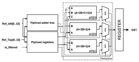
Figure 16. Hardware architecture of DC Prediction.

In special cases with predicted samples at positions $p\left[0\right]\left[0\right]$, $p\left[x\right]\left[0\right]$, and $p\left[0\right]\left[y\right]$, when the dcVal value is ready, it is put inside three-taps ($p\left[0\right]\left[0\right]$) or two-taps filter module ($p\left[x\right]\left[0\right]$ and $p\left[0\right]\left[y\right]$), a multiplexer set is added to these values with control signal is a $is\_filter$ variable. In the case $is\_filter=1$, the output value equals $dcVal$ after processing through filters. Vice versa, if $is\_filter=0$, the final value is $dcVal$. The first output requires seven clock cycles to complete all pipeline registers, and the next projected value is ready at each cycle.

4. Functional Verification

To validate our solution, we create a Universal Verification Methodology (UVM) environment, as illustrated in Figure 17. The Angular, DC, and Planar sequences are randomized and delivered to DUT via a virtual interface. The DUT output is gathered and monitored before being compared to the output of the H.265/HEVC intra-prediction software reference model and updated in the coverage report.

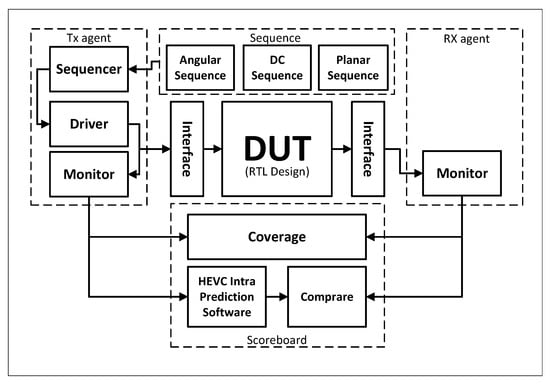
Figure 17. The structure of the verification environment used for our DUT.

An open-source H.265/HEVC encoder [11] is used as a reference model for the intra-prediction module in this research. The model was created in the C programming language and supports all intra-prediction modes and PU sizes. By employing the SystemVerilog Direct Programming Interface [12] (DPI), which allows SystemVerilog to connect directly with functions written in C, we can eliminate errors in constructing our own software reference model because we reuse existing C functions from [11].

Questasim 10.7c is used to operate our test environment. A test case is considered “PASSED” when the same input reference sample is used, and the prediction output of the DUT with the software model is the same. We set coverage checkpoints for all prediction modes to ensure that our design was covered during the simulation phase. The simulation results indicate that our design function was successful.

5. Synthesis Results

The proposed hardware architecture is described in SystemVerilog, with a synthesis target of Xilinx Virtex-7 (xc7vx485tffg1761-3) and a speed grade = −2.

The latencies of the PU modules taken to perform in a CU module are described in Table 3. The parameters Latency of load reference samples, Latency of reconstruction loop, Latency of sample prediction, and Number PUs in 1 CU are labeled by (1), (2), (3), and (4). For the PU $4\times 4$, PU 8 × 8, PU $16\times 16$, and PU $32\times 32$, the latencies of loading reference samples are 1, 1, 2, and 4, respectively. As shown in Figure 2, the latencies of the reconstruction loop of those PUs are the delay from the Sample Prediction unit, Subtraction, Transform, Quantization, Inverse Quantization, Inverse transform, and Summation modules. For the optimal pipelined design, the delay of the Subtraction, Transform, Quantization, Inverse Quantization, Inverse transform, and Summation modules can be estimated by 1, 2, 2, 2, 2, and 1 cycles, respectively. The latencies of the Sample Prediction unit are 3, 3, 36, and 36 clocks for the PU $4\times 4$, PU 8 × 8, PU $16\times 16$, and PU $32\times 32$, respectively. Therefore, the latencies of the reconstruction loop of those PUs are 13, 13, 46, and 46, respectively. For the worst-case prediction for one CU module, 1 PU $32\times 32$, 4 PUs $16\times 16$, 16 PUs 8 × 8, and 64 PUs $4\times 4$ are performed. Then, the total latency to finish one CU module is 546 cycles. Therefore, as shown in Table 4, if we do the intra-prediction for the FHD frame, there are 2020 CU modules to be executed. Then, the frame rate is 210 FPS. If we do the intra-prediction for the 4K frame, there are 8100 CU modules to be executed. Then, the frame rate is 52 FPS.

Table 3. Latency of PUs processing in a CU.

PU Size	Lat. of Load Ref. Samples (No. Clocks) (1)	Lat. of RL (No. Clocks) (2)	Lat. of Sample Prediction (No. Clocks) (3)	No. PUs in 1 CU (4)	Lat. of PUs in 1 CU (No. Clocks) (1) + (2) + (3) × (4)
4 × 4	1	13	3	64	206
8 × 8	1	13	3	16	62
16 × 16	2	46	36	4	192
32 × 32	4	46	36	1	86
Lat. of 1 CU (No. Clocks)					546

Table 4. Frame Rate of the FHD and 4K Video.

Frame	No. CUs	Lat. of 1 CU (No. Clocks)	Lat. of 1 frame (No. Clocks)	Freq. (MHz)	Frame Rate (FPS)
FHD	2020	546	1,102,920	232	210
4K	8100	546	4,422,600	232	52

The synthesis comparison results are shown in Table 5 and Table 6. The slide LUTS utilization costs 73%, and the slice registers utilization costs 41% of the FPGA resources. The memory utilization of our design is high because all reconstructed samples are stored in register buffers, including the original buffer, reference buffer, and control buffer, as shown in Figure 5.

Table 5. Synthesis results and comparison with the other FPGA implementations.

	[13]	[14]	[15]	[16]	[17]	[18]	[2]	This Work
Technology	Arria-II	ZCU-120	Arria-II	Stratix-V	Stratix-V	Kintex-7	Virtex-7	Virtex-7
PU size	4; 8;	4; 8;	4; 8;	4; 8;	4; 8;	4; 8;	4; 8;	4; 8;
	16; 32	16; 32	16; 32	16; 32	16; 32	16; 32	16; 32	16; 32
LUTs	31,179	49,678	83,548	195,883	201,823	63,450	170,000	214,000
Registers	N/A	36,214	N/A	N/A	N/A	19,430	110,000	220,000
Freq (MHz)	100	200	140	120	120	175	256	232
FHD Frame rate (FPS)	17.52	29	30	45	45	60	110	210
4K Frame rate (FPS)	4.38	7.25	7.5	11.25	11.25	15	24	52
Bitrate/Area (Kbps/LUT)	27.96	29.05	17.87	11.43	11.1	47.06	28.10	48.37
Compress ratio	N/A	N/A	N/A	NA	NA	N/A	N/A	242.94

Table 6. Synthesis results and comparison with the other FPGA implementations (continue).

	[19]	[20]	[21]	[22]	This Work
Technology	Arria-10	Zynq-7000	Arria-II	Arria-10	Virtex-7
PU size	4; 8;	4; 8;	4; 8;	4; 8;	4; 8;
	16; 32	16; 32	16; 32	16; 32	16; 32
LUTs	552,000	8698	93,184	308,000	214,000
Registers	N/A	9852	481	N/A	220,000
Freq (MHz)	175	200	100	125	232
FHD Frame rate (FPS)	240	8	60	120	210
4K Frame rate (FPS)	60	2	15	30	52
Bitrate/Area (Kbps/LUT)	21.64	45.82	32.04	19.39	48.37
Compress ratio	N/A	N/A	N/A	NA	242.94

Compared to earlier works, the proposed design [13] accelerates the throughput of the most frequently used PU (PU $4\times 4$). This approach provides a frame rate of 4.38 FPS for the 4K resolution. To increase the throughput up to 7.5 FPS, the authors of [14,15] applied the pipelined TU coding and the paralleled intra-prediction architectures. By applying a fully parallel manner for the mode prediction, transformation, quantization, inverse quantization, inverse transformation, rate estimation, and reconstruction processes, [16,17] provided a frame rate of 11.25 FPS. To improve both throughput and hardware resources, ref. [18] proposed a four-stage pipeline architecture. This approach provides a frame rate of 15 FPS with a high bit rate/area (47 Kbps/LUT). To reach real-time 4K video processing of 24 FPS, [2] simplified the equations of all calculations for reference sample preparations and applied parallel computing. The authors of [19,22] investigated parallelization of Kvazaar-based intra-encoder on CPU and FPGA platforms to obtain the frame rate of 60 FPS for the 4K resolution with a bit rate/area of about 20 Kbps/LUT. The authors of [20] studied the impact of a high-level synthesis (HLS) design method on the HEVC intra-prediction block decoder. Although this work provides a high bit rate/area (45.82 Kbps/LUT), the frame rate is only 2 FPS. To increase the frame rate of 15 FPS, [21] proposed the computationally scalable algorithm and the architecture design for the H.265/HEVC intra-encoder. This design provides a bit rate/area of 32.04 Kbps/LUT. The designs in [23,24] provide a high frame rate of 30 FPS for the 4K resolution. However, the hardware resources of these works are not mentioned. To extremely reduce the hardware resources, some works applied approximation algorithms to simplify the designs [3,4,25,26]. The frame rates of those designs are 10, 13.75, 30, and 24 FPS, respectively. Although these approaches helped to increase the bit rate/area performance extremely, their peak signal-to-noise ratios (PSNRs) are affected. In addition to implementing on FPGA platforms, some works are designed and implemented on the ASIC platform [27,28] to provide the frame rate of 30 FPS for the 8K resolution. As shown in Table 5 and Table 6, our work provides a frame rate of 52 FPS with a high bit rate/area (48 Kbps/LUT). This throughput is high enough for the real-time processing of the 4K video frame.

6. Conclusions

This research uses both DSP and non-DSP versions of H.265/HEVC intra-prediction. PEA and PEP cells were employed to reduce the complexity of multiplications by developing a pipeline design with parallel processing for DC, Angular, and Planar predictions. The architecture creates multiple predictions for the angular mode with PU sizes of $4\times 4$ and $8\times 8$ with the flexible use of PEA cells. The design was synthesized and mapped to the Xilinx Virtex-7, which can handle 210 FPS for the FHD resolution and 52 FPS for the 4K resolution. The design is appropriate for high-resolution real-time coding. However, the hardware resources of our design still need to be improved. In future work, we will explore the approximation techniques to apply to our current design to optimize hardware resources and accuracy.

References

- Kalali, E.; Adibelli, Y.; Hamzaoglu, I. A high performance and low energy intra prediction hardware for High Efficiency Video Coding. In Proceedings of the 22nd International Conference on Field Programmable Logic and Applications (FPL), Oslo, Norway, 29–31 August 2012; pp. 719–722. [Google Scholar] [CrossRef]
- Amish, F.; Bourennane, E.-B. Fully pipelined real time hardware solution for High Efficiency Video Coding (HEVC) intra prediction. J. Syst. Archit. 2016, 64, 133–147. [Google Scholar] [CrossRef]
- Azgin, H.; Kalali, E.; Hamzaoglu, I. A computation and energy reduction technique for HEVC intra prediction. IEEE Trans. Consum. Electron. 2017, 63, 36–43. [Google Scholar] [CrossRef]
- Azgin, H.; Mert, A.C.; Kalali, E.; Hamzaoglu, I. An efficient FPGA implementation of HEVC intra prediction. In Proceedings of the 2018 IEEE International Conference on Consumer Electronics (ICCE), Las Vegas, NV, USA, 12–14 January 2018; pp. 1–5. [Google Scholar] [CrossRef]
- Sullivan, G.J.; Ohm, J.; Han, W.; Wiegand, T. Overview of the High Efficiency Video Coding (HEVC) Standard. IEEE Trans. Circuits Syst. Video Technol. 2012, 22, 1649–1668. [Google Scholar] [CrossRef]
- Wang, C.; Kao, J.-Y. Fast Encoding Algorithm for H.265/HEVC Based on Tempo-spatial Correlation. Int. J. Comput. Consum. Control. (IJ3C) 2015, 4, 51–58. [Google Scholar]
- Lainema, J.; Bossen, F.; Han, W.J.; Min, J.; Ugur, K. Intra Coding of the HEVC Standard. IEEE Trans. Circuits Syst. Video Technol. 2012, 22, 1792–1801. [Google Scholar] [CrossRef]
- Zhang, X.; Liu, S.; Lei, S. Intra mode coding in HEVC standard. In Proceedings of the 2012 Visual Communications and Image Processing, San Diego, CA, USA, 27–30 November 2012; pp. 1–6. [Google Scholar] [CrossRef]
- Nair, P.S.; Nair, M.S. On the analysis of HEVC Intra Prediction Mode Decision Variants. Procedia Comput. Sci. 2020, 171, 1887–1897. [Google Scholar] [CrossRef]
- Xilinx. 7 Series DSP48E1 Slice User Guide. UG479 (v1.10). 27 March 2018. Available online: https://docs.xilinx.com/v/u/en-US/ug479_7Series_DSP48E1 (accessed on 1 February 2023).
- Viitanen, M.; Koivula, A.; Lemmetti, A.; Ylä-Outinen, A.; Vanne, J.; Hämäläinen, T.D. Kvazaar: Open-Source HEVC/H.265 Encoder. In Proceedings of the 2016 ACM International Conference on Multimedia (MM’16), New York, NY, USA, 15–19 October 2016; pp. 1179–1182. [Google Scholar] [CrossRef]
- 1800-2017–IEEE Standard for SystemVerilog–Unified Hardware Design, Specification, and Verification Language; IEEE: Piscataway, NJ, USA, 2018. [CrossRef]
- Abramowski, A.; Pastuszak, G. A double-path intra prediction architecture for the hardware H.265/HEVC encoder. In Proceedings of the 17th International Symposium on Design and Diagnostics of Electronic Circuits & Systems, Warsaw, Poland, 23–25 April 2014; pp. 27–32. [Google Scholar] [CrossRef]
- Chen, W.; He, Q.; Li, S.; Xiao, B.; Chen, M.; Chai, Z. Parallel Implementation of H.265 Intra-Frame Coding Based on FPGA Heterogeneous Platform. In Proceedings of the 2020 IEEE 22nd International Conference on High Performance Computing and Communications; IEEE 18th International Conference on Smart City; IEEE 6th International Conference on Data Science and Systems (HPCC/SmartCity/DSS), Yanuca Island, Cuvu, Fiji, 14–16 December 2020; pp. 736–743. [Google Scholar] [CrossRef]
- Atapattu, S.; Liyanage, N.; Menuka, N.; Perera, I.; Pasqual, A. Real time all intra HEVC HD encoder on FPGA. In Proceedings of the 2016 IEEE 27th International Conference on Application-specific Systems, Architectures and Processors (ASAP), London, UK, 6–8 July 2016; pp. 191–195. [Google Scholar] [CrossRef]
- Zhang, Y.; Lu, C. High-Performance Algorithm Adaptations and Hardware Architecture for HEVC Intra Encoders. IEEE Trans. Circuits Syst. Video Technol. 2019, 29, 2138–2145. [Google Scholar] [CrossRef]
- Zhang, Y.; Lu, C. Efficient Algorithm Adaptations and Fully Parallel Hardware Architecture of H.265/HEVC Intra Encoder. IEEE Trans. Circuits Syst. Video Technol. 2019, 29, 3415–3429. [Google Scholar] [CrossRef]
- Ding, D.; Wang, S.; Liu, Z.; Yuan, Q. Real-Time H.265/HEVC Intra Encoding with a Configurable Architecture on FPGA Platform. Chin. J. Electron. 2019, 28, 1008–1017. [Google Scholar] [CrossRef]
- Sjövall, P.; Viitamäki, V.; Vanne, J.; Hämäläinen, T.D.; Kulmala, A. FPGA-Powered 4K120p HEVC Intra Encoder. In Proceedings of the 2018 IEEE International Symposium on Circuits and Systems (ISCAS), Florence, Italy, 27–30 May 2018; pp. 1–5. [Google Scholar] [CrossRef]
- Atitallah, A.B.; Kammoun, M. High-level design of HEVC intra prediction algorithm. In Proceedings of the 2020 5th International Conference on Advanced Technologies for Signal and Image Processing (ATSIP), Sousse, Tunisia, 2–5 September 2020; pp. 1–6. [Google Scholar] [CrossRef]
- Pastuszak, G.; Abramowski, A. Algorithm and Architecture Design of the H.265/HEVC Intra Encoder. IEEE Trans. Circ. Syst. Video Tech. 2015, 26, 210–222. [Google Scholar] [CrossRef]
- Sjövall, P.; Viitamäki, V.; Oinonen, A.; Vanne, J.; Hämäläinen, T.D.; Kulmala, A. Kvazaar 4K HEVC intra encoder on FPGA accelerated airframe server. In Proceedings of the 2017 IEEE International Workshop on Signal Processing Systems (SiPS), Lorient, France, 3–5 October 2017; pp. 1–6. [Google Scholar] [CrossRef]
- Aparna, P. Efficient Architectures for Planar and DC modes of Intra Prediction in HEVC. In Proceedings of the 2020 7th International Conference on Signal Processing and Integrated Networks (SPIN), Noida, India, 27–28 February 2020; pp. 148–153. [Google Scholar] [CrossRef]
- Shastri, S.; Lakshmi; Aparna, P. Complexity Analysis of Hardware Architectures for Intra Prediction unit of High Efficiency Video Coding (HEVC). In Proceedings of the 2020 International Conference on Electronics, Computing and Communication Technologies (CONECCT), Bangalore, India, 2–4 July 2020; pp. 1–6. [Google Scholar] [CrossRef]
- Min, B.; Xu, Z.; Cheung, R.C. A Fully Pipelined Hardware Architecture for Intra Prediction of HEVC. IEEE Trans. Circ. Syst. Video Tech. 2016, 27, 2702–2713. [Google Scholar] [CrossRef]
- Kalali, E.; Hamzaoglu, I. An Approximate HEVC Intra Angular Prediction Hardware. IEEE Access 2019, 8, 599–2607. [Google Scholar] [CrossRef]
- Tang, G.; Jing, M.; Zeng, X.; Fan, Y. A 32-Pixel IDCT-Adapted HEVC Intra Prediction VLSI Architecture. In Proceedings of the 2019 IEEE International Symposium on Circuits and Systems (ISCAS), Sapporo, Japan, 26–29 May 2019; pp. 1–5. [Google Scholar] [CrossRef]
- Fan, Y.; Tang, G.; Zeng, X. A Compact 32-Pixel TU-Oriented and SRAM-Free Intra Prediction VLSI Architecture for HEVC Decoder. IEEE Access 2019, 7, 149097–149104. [Google Scholar] [CrossRef]
Disclaimer/Publisher’s Note: The statements, opinions and data contained in all publications are solely those of the individual author(s) and contributor(s) and not of MDPI and/or the editor(s). MDPI and/or the editor(s) disclaim responsibility for any injury to people or property resulting from any ideas, methods, instructions or products referred to in the content. |
© 2023 by the authors. Licensee MDPI, Basel, Switzerland. This article is an open access article distributed under the terms and conditions of the Creative Commons Attribution (CC BY) license (https://creativecommons.org/licenses/by/4.0/).