The Prior Model-Guided Network for Bearing Surface Defect Detection

Abstract

Surface defect detection is a key task in industrial production processes. However, the existing methods still suffer from low detective accuracy to pit and small defects. To solve those problems, we establish a dataset of pit defects and propose a prior model-guided network for defect detection. This network is composed of a segmentation network with a weight label, classification network, and pyramid feature fusion module. The segmentation network as the prior model can improve the accuracy of the classification network. The weight label with center distance transformation can reduce the label cost of the segmentation network. The pyramid feature fusion module can adapt defects of different scales and avoid information loss of small defects. The comparison experiments are implemented to identify the performance of the proposed network. Ablation experiments are designed to specify the effectiveness of every module. Finally, the network is performed on a public dataset to verify its robustness. Experimental results reveal that the proposed method can effectively identify pit defects of different scales and improve the accuracy of defect detection. The accuracy can reach 99.3%, which is increased by 2~5% compared with other methods, revealing its excellent applicability in automatic quality inspection of industrial production.

1. Introduction

Bearing, as one of the most widely used mechanical basic parts in the world, is considered “the joint of modern mechanical industry” to enable the efficient operation of mechanical equipment [1]. Most scenarios of bearing usage are complicated environments, including outdoor sites, production workshops, and construction places. If any external object enters the bearing raceway or roller gap, the work of bearings can be largely affected and even mechanical paralysis can be triggered, which may result in unimaginable safety accidents. Therefore, the presence of the bearing covers offers a favorable solution to this problem. The use of the bearing cover can isolate the bearing from the external environment, protect the bearing from rusting and corrosion, and prevent the lubricant from leaking, thus can prolong the life of the bearing. During the bearing manufacturing process, the bearing cover is the weakest part, and the surface often generates many pits, which there is a potential danger. Therefore, the final quality detection process is indispensable in the production process. However, quality detection still relies on manual operation in the factory, which has low efficiency and high cost. With the introduction of the industry 4.0 model, algorithms based on deep learning have been adopted to solve industry problems [2,3,4,5,6,7]. However, pit defect detection of bearing production based on the method is still a vacancy need to be studied urgently.

When collecting images of bearings, the images are easily affected by the light changes due to the property of metal materials. Moreover, the surface of the bearing cover is not flat, which may cause noise in the collected data. There exist many challenges in the pit defects detection on metal bearing cover surfaces: (1) Large differences within the class. Due to the particularity of the bearing material, the data collected by different bearings with the same material shows an obvious difference as shown in Figure 1a. (2) Diversification of defects. Pit defects on the bearing cover have various shapes and sizes as shown in Figure 1b,c. (3) Weak features of small defects. Small defects account for a small proportion of the overall area, so the contrast is relatively low, and the defect features are not obvious as shown in Figure 1c.

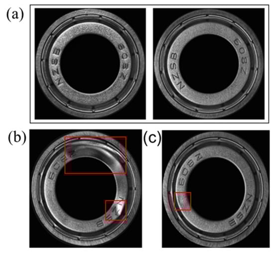
Figure 1. Challenges of bearing inspection from the industry. (The surface defect of the bearings is in the red box) (a) The data of two non-defective bearings exhibit large surface differences. (b) Defects of different sizes. (c) Small defects.

For the large differences within the class, the model needs to effectively learn the detailed features of the object. In this paper, the segmentation network is used as the prior model, and the resulting map of the segmentation network is used to guide the classification network. Through fine-grained classification, the detailed features of the same category can be better learned. For the problem of diverse defects and weak features of small defects, the model needs to remain robust against various changes in the defect. The most commonly used methods based on convolutional neural networks (CNN) tend to expand the network’s receptive field to cover the entire defect of target objects. Different feature layers of CNN have different sensitivity to objects. Low-level features with higher resolution can generate clear and detailed boundaries but lack contextual information. While high-level features have more abstract semantic information and are good at category classification, but weaker in shape recognition and location [8,9,10,11]. Nowadays, these methods mainly focus on the high-level features extracted from the deep layer of the network. Since CNN uses pooling layers repeatedly to extract advanced semantics, the pixels of small objects can be filtered out during the downsampling process, thus resulting in poor recognition of small defects [12].

Feature pyramid networks can solve the small target problem well [13,14]. This paper introduces the pyramid feature fusion module (PFFM) [15], which crosses the fusion of the features of different stages to fully obtain context information, thereby avoiding the loss of small defect information, and can well extract the features of different size defects. The final segmentation result map is obtained by passing the extracted features through the 1 × 1 convolution kernel and then used as the attention map. Then, global feature extraction is performed on the attention map, which is used as the prior knowledge of the classification network to improve the accuracy of defect recognition. The main contributions are as follows.

(1)

A prior model-guided network (PMG-Net) was proposed for defect detection, which uses the segmentation network as the prior model to guide the classification network to better learn the features of objects. And a pyramid feature fusion module is introduced in the segmentation network to fully combine context information. This improves the classification accuracy of the proposed method.

(2)

To verify the performance of the proposed method, we established a large-scale dataset of pit defects on the bearing cover surfaces in real industrial scenarios for deep learning.

(3)

The center distance transformation formula acted as the weight label was introduced to the segmentation network to reduce the label cost.

The rest of this paper is organized as follows. Section 2 presents related work on surface defects detection. Next, the proposed PMG-Net is described in detail in Section 3. Subsequently, Section 4 describes the acquisition of the dataset, with an evaluation and corresponding discussion of the proposed method. Finally, Section 5 summarizes this article.

2. Related Works

Recently, surface defects detection methods based on computer vision can be divided into traditional detection methods and deep learning-based detection methods.

2.1. Traditional Method

Liu et al. [16] applied a multi-angle illumination method to collect images of the pits and scratches on the surface of the bearing cover. The pits and scratches detection was realized through polar coordinate transformation and optimized OTSU threshold. One bearing surface needs to be identified eight times with light sources of eight angles, so the efficiency is considerably low. Shen et al. [17] designed a self-comparison method to replace the template comparison method for bearing cover defects detection. This method has a low error tolerance rate for image acquisition, and the efficiency cannot meet the detection requirements. Mien et al. [18] proposed a new wavelet kernel function to construct the kernel function of Linear local fisher discriminant analysis to extract effective features for bearing defect classification. The method is effective in seeking the optimized parameters but performs poorly in detection. Pacas et al. [19] constructed a dynamic threshold algorithm to detect surface defects of bearing steel balls by using the probability density function of the data distribution. Chen et al. [20] reconstruct the global image based on discrete cosine transformation, which can restore defect regions in the image by setting a threshold and be applied in tiny surface defects detection. Although these traditional techniques have achieved good performance in defect detection, the heavy reliance on expert knowledge and poor robustness hinder their wild application.

2.2. Deep Learning

Several related works have explored the application of deep learning in industrial anomaly detection and classification [21,22,23,24], but there are very few studies on the defect detection of bearing cover. The unsupervised method only requires normal samples and does not require a defect label, most methods are now unsupervised. Haselmann et al. [25] designed a fully convolution-based auto-encoding network to detect surface defects on decorative plastic parts. Youkachen et al. [26] used a convolutional autoencoder for image reconstruction and obtained the final surface defect segmentation results of hot-rolled strip steel. Zhai et al. [27] adopted a multi-scale fusion strategy to fuse the responses of the three convolutional layers of the GAN discriminator, and then used the Otsu method to further segment defect locations on the fused feature correspondence map. These above-mentioned unsupervised methods learn the features of normal samples, and judge whether the samples are defective by comparing the feature differences between the two images.

The bearing data is collected by multi-angle point light sources, and the bearing angle of the collection process will change due to equipment reasons, so it is difficult for unsupervised methods to learn the differences between bearings. We tried the latest unsupervised methods of Patchcore [28], Padim [29], and Cflow [30], and some of the results are shown in Figure 2. From the resulting image, it can be found that the unsupervised method is not suitable for complex industrial scenes. These methods are susceptible to changes in illumination and positions, making the network misjudge the position changes of characters as abnormal areas, resulting in low recognition accuracy.

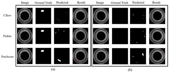
Figure 2. The result of defect detection with unsupervised methods. (a) the resulting image for defective data; (b) the resulting image for non-defective data.

However, in actual industrial applications, there are still supervision methods to detect defects. Yang et al. [31] applied YOLOv5 to steel pipe weld defect detection. Cha et al. [32] detected bridge defects based on the two-stage detector Faster R-CNN, where the backbone network was replaced by ZF-Net to improve real-time performance. Zhou et al. [33] apply a novel anchor mechanism to generate suitable candidate boxes for objects and combine multi-level features to construct discriminative features for split pins defect inspection. Recently, one group [34] studied the defects detection of rubber bearing cover, achieving good results in detecting the surface defects of the bearing rubber seal cover by modifying the YOLOv3 network. But the classification confidence of some images still needs to be improved.

3. Methods

In this section, we give an overview of PMG-Net, and then illustrate every module used to build this network.

3.1. Overview

As shown in Figure 3, PMG-Net is composed of the segmentation network and the classification network. The segmentation network concludes the multilevel features extraction module (MFEM) and the pyramid feature fusion module. The classification network contains the classification backbone and the segmentation result map.

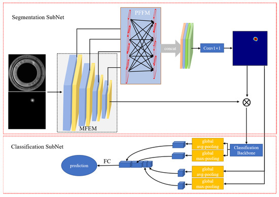
Figure 3. Details of the proposed PMG-Net. First input the image to extract the features of different stages in MFEM. Then, the extraction feature is then passed through the PFFM module fusion features, and the features adjustment dimension after 1 × 1 convolution will be fused to obtain the segmentation result. The segmentation results are multiplied with the last layer of MFEM to get enhanced features as the input of the classification network. Finally, the features by the classification backbone are extracted and segmentation results are sent to the full connection layer through the global average and maximum pooling, and the final prediction results are obtained.

During the working process, a batch of original images with the same resolution and their corresponding weight labels are input into the PMG-Net first. Then, features of different scales in four stages are extracted through the MFEM. Afterward, the extracted features pass through the PFFM to generate multi-scale global contextual features and extract rich contextual information. The obtained global contextual features are channel fused, using 1 × 1 convolution to adjust the channel dimension of the feature to get the final segmentation result map. Finally, the segmentation result map is multiplied pixel by pixel with the features of the last stage of the MFEM to obtain the enhanced features. The final segmentation result map with the defective location acts as the prior knowledge of the classification network and assists the classification network for image recognition. Meanwhile, the enhanced features are inputted into the classification backbone to further extract features. The extracted features and the final segmentation result map are used in the channel dimension to gain the output neurons by global average pooling and global maximum pooling. The output neurons are inputted into the fully connected layer to get the final prediction result.

3.2. Multilevel Features Extraction Module (MFEM)

CNN is widely used for feature extraction of objects, which are learned by stacking multiple convolution kernels and pooling layers [35]. In this paper, the MFEM includes four layers of shallow, fine, deep, and rough, layers. From the shallow and fine layers, original features and low-level features of the image (such as edges and contours) can be acquired; From the deep and rough layers, deep abstract semantic features of the image can be found [15]. Every layer consists of max pooling and convolutional blocks with different amounts, and each convolutional block consists of a convolutional kernel (Conv), rectified linear unit (ReLu) activation function, and batch normalization (BN). The details of MFEM can be found in Table 1.

Table 1. Details of multi-scale feature extraction module.

Layer	Type
Input	C = 1
Layer1	[Conv 5 × 5 + BN + ReLu, C = 32] × 2 max pooling 2 × 2
Layer2	[Conv 5 × 5 + BN + ReLu, C = 64] × 3 max pooling 2 × 2
Layer3	[Conv 5 × 5 + BN + ReLu, C = 128] × 4 max pooling 2 × 2
Layer4	[Conv 5 × 5 + BN + ReLu, C = 256] × 2 max pooling 2 × 2

3.3. Pyramid Feature Fusion Module (PFFM)

When using MFEM, deep and advanced features can be extracted from the network. The area of small defects only accounts for a small part of the entire image, and as the depth of the network increases, the feature information will be lost, which will make the small defect feature information weaker. Therefore, PFFM is introduced to compensate for this shortcoming as shown in Figure 4. It can generate a multi-scale global contextual feature and extract rich contextual information.

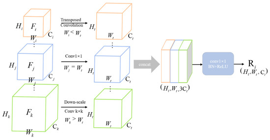
Figure 4. Details of PFFM module. The features obtained from MFEM are adjusted to the same dimension as the target resolution by transposed convolution, conv operation, and down-scale. Then, feature cross-fusion maps at different stages are obtained using channel fusion and 1 × 1 convolution.

The image with a resolution of W × H is passed through the MFEM to obtain multi-scale features of different layers. The features of the four layers are represented by the feature set F: F = ($F_1$,$F_2$,$F_3$,$F_4$), where F1 represents the features that have passed through Layer1, and so on. To make full use of the context information, the features of different layers are mapped to feature maps of different resolutions: $I_n$ = ($W/2^{n-1}-$,$H/2^{n-1}$), where n = (1,2,3,4), W and H represent the width and height of the input image, respectively. The feature $F_1$ with the resolution of $I_1$ was reduced to different resolutions by using convolution kernels with different sizes. The output features $O_1^i$ are as follows:

$$O_1^i={ℳ}_{down-scale}\left(F_1\right)=\sigma \left(BN\left(W_{k\times k,s}\ast F_1\right)\right)\left(i=1,\dots ,4\right),$$

(1)

where $\sigma$ represents the ReLu, $W_{k\times k,s}$ represents the convolution with the $k\times k$ convolution kernel and stride of $s$, and $\ast$ represents the convolution operation. For the feature obtained by Layer4 for $F_4$, its resolution $I_4$ is the smallest, which is upsampled into features of different resolutions through transposed convolution. Its output features $O_4^i$ are as follows:

$$O_4^i={ℳ}_{upsample}\left(F_4\right)=\sigma \left(BN\left(W_{k\times k,s}{}^T\ast F_4\right)\right)\left(i=1,\dots ,4\right)$$

(2)

where $W_{k\times k,s}{}^T$ represents Transposed Convolution with the $k\times k$ convolution kernel and stride of $s$. For $F_2$ and $F_3$ whose resolutions are between $I_1$ and $I_4$, a combination of upsampling and downscaling is used to map them to the resolution of different features. Its output features $O_b^i$ are as follows:

$$O_b^i={ℳ}_{down-scale}\left(F_b\right)\&{ℳ}_{upsample}\left(F_b\right)\left(i=1,\dots ,4;b=2,3\right)$$

(3)

where ${ℳ}_{down-scale}$ and ${ℳ}_{upsample}$ represent Equations (1) and (2). These adjusted feature maps ($O_1^i$,…,$O_4^i$) have a channel dimension of 128. Finally, these feature maps with the same resolution are fused to generate the final four fused feature maps, named $R_i$, defined as:

$$R_i=\sigma (BN(W_{1\times 1}\ast CAT(O_1^i, \dots , O_4^i)))\left(i=1,\dots ,4\right),$$

(4)

where $CAT$ represents channel fusion, that is, channel splicing. $W_{1\times 1}$ represents the 1 × 1 convolution kernel, which changes the channel dimension of features. The fused channels are adjusted from 512 dimensions to 128 dimensions, and the fused features $R_i$ are downscaled to $I_4$ resolution features. Four different resolutions are merged again, and the channel dimension of the feature map is adjusted using 1 × 1 convolution to obtain the final segmentation result map $S$, which is defined as follows:

$$Y_i={ℳ}_{downscale}\left(R_i\right)\left(i=1,\dots ,4\right)$$

(5)

$$S=\sigma (BN(W_{1\times 1}\ast CAT(Y_1,Y_2,Y_3,Y_4))),$$

(6)

The fused feature dimension after the use of 1 × 1 convolution is adjusted from 512 dimensions to 1 dimension as the final segmentation result map. All parameters are shown in Table 2. Through this multi-scale information cross-fusion, the information of different stages is effectively obtained, thereby avoiding the loss of information in deep features.

Table 2. Details of the pyramid cross-fusion module.

Stage	R1	R2	R3	R4
Layer 1	D: 1 × 1, s = 1	D: 2 × 2, s = 2	D: 4 × 4, s = 4	D: 8 × 8, s = 8
Layer 2	T: 2 × 2, s = 2	D: 1 × 1, s = 1	D: 2 × 2, s = 2	D: 4 × 4, s = 4
Layer 3	T: 4 × 4, s = 4	T: 2 × 2, s = 2	D: 1 × 1, s = 1	D: 2 × 2, s = 2
Layer 4	T: 8 × 8, s = 8	T: 4 × 4, s = 4	T: 2 × 2, s = 2	D: 1 × 1, s = 1

D means down-scale, which is the Conv; T means upsample, which is the Transposed Convolution.

3.4. Weight Label

The segmentation network is a fine-grained classification network, which classifies each pixel in the image, so fine labels are required as the ground truth, leading to high labeling costs. To solve this problem, this paper proposes the weight label, which means the positions of different pixels in the defect area are assigned different weights. Most of the surface defects of the bearing cover are pits, so more attention should be paid to the central part of the labeled area, and less attention to the peripheral part.

The image of the bearing cover is shown in Figure 5a. The region of interest (Figure 5b) is extracted from Figure 5a by the EDCircle method [36]. Figure 5c is obtained from Figure 5a by the annotation software Labelme. It is obvious that only the shape of the rectangular frame is labeled. Then, taking the intersection of Figure 5b,c, the semi-fine label can be acquired as shown in Figure 5d. Afterward, we can find the center point of Figure 5d and assign different weights to different pixels according to the distance from the pixels to the center point. The weight of the center point is 1. And the closer to the center point, the higher the weight is. The weights of pixels are calculated as follows:

$$P_{weight}\left(pix\right)=\omega \ast {\left(\frac{D{\left(pix\right)}_{max}-D\left(pix\right)}{D{\left(pix\right)}_{max}}\right)}^{\alpha }$$

(7)

where $pix$ represents each pixel in the annotated area, $D{\left(pix\right)}_{max}$ represents the farthest distance from the center point, and $D\left(pix\right)$ represents the distance from each pixel to the center point. $\alpha$ controls the rate at which the importance of pixels decreases as they move farther away from the center point. $\omega$ is an additional scalar weight to control the interval between the importance of pixels. Note that the weight of all non-annotated regions remains 1. This is because when training a non-defect image, all the pixels in the label are set as negative sample pixels, which are used to train the segmentation network and enhance the generalization of the network.

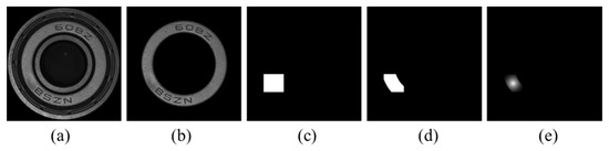
Figure 5. The weight label for segmentation networks. (a) original image; (b) region of interest; (c) annotation label; (d) semi-fine label; (e) weight label.

3.5. Classification Subnet Module

Segmentation network training with weight labels may lead to overfitting on non-defect images. The labeling process uses a rectangular frame for labeling, which will generate a lot of useless information. Although the weight label is used and the edge information is set to a small weight, it is inevitable that the network will learn the edge information as the positive sample pixel. That will cause some non-defect images to be identified as defective, resulting in overfitting. To this end, the classification subnet is added to adjust the pixel information of the peripheral weight, and the image-level label is used to adjust the insufficiency of the pixel-level weight label. Figure 6 shows the details of the classification subnet. The segmentation result map, which can increase the weight of important regions, multiplies the last layer features of MFEM by elements, and the results act as input (1024 channels) to the classification backbone. The classification backbone consists of multiple stacked convolutional layers, and the convolutional layer outputs are 256, 64, and 16 channels, respectively. The features obtained from the backbone structure and the final segmentation result map are subjected to global average and global maximum pooling to generate 34 output neurons, and these neurons are passed through the fully connected layer to obtain the final output confidence.

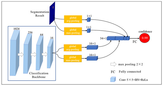
Figure 6. Details of classification subnet. The segmentation result and classification backbone features obtained neurons by the global average and maximum pooling, and the obtained neurons are sent to the full connection layer to obtain the final prediction value.

The segmentation result map is used as the prior knowledge can provide important information about the defective location and guide the classification subnet for training. The classification subnet guarantees the adaptability to large and complex shapes through multi-layer convolution and downscale. The global average and the global maximum pooling of the last layer of the classification backbone and the segmentation result map are used as the input of the full connection layer, which can strengthen the guidance of prior knowledge and avoid using a large amount of unnecessary feature information. Thus, the PMG-Net can not only capture local shapes, but also capture global shapes spanning large areas of the image, which can identify the defects of different shapes.

3.6. Training Constraints

In the training process, the segmentation network and the classification subnet are trained at the same time, so that the weight labels can be better used. Segmentation and classification losses are combined into a single unified loss for simultaneous learning in an end-to-end manner [37]. Loss is defined as follows:

$${ℒ}_{seg}={ℒ}_{cls}=-\frac{1}{N}{\sum }_{i=1}^N\left[y_i\log P_i+(1-y_i\right)\log (1-P_i)]$$

(8)

$$ℒ=(1-\frac{n}{n_{ep}})·P_{weight}\left(pix\right)·{ℒ}_{seg}+\frac{n}{n_{ep}}·{ℒ}_{cls}$$

(9)

where n represents the number of current epochs, $n_{ep}$ represents the total number of epochs, $P_{weight}\left(pix\right)$ represents Equation (7), $y_i$ represents the true probability of the i-th image, $P_i$ represents the predicted probability of the i-th image, and N represents the batch size. Through $n/n_{ep}$ we control the focus on learning different networks. In the initial stage of training, the segmentation network has not yet produced meaningful output. Using the results of the segmentation network to guide the classification will lead to a decline in the results. Therefore, in the early stage, we only learn the segmentation network, and then gradually transition to only learning the classification subnet.

4. Experiment

In this section, we introduce the datasets in detail and evaluate the performance of the proposed method as well as some implementation details.

4.1. Dataset

4.1.1. Bearing Dataset

For the detection of surface defects on metal bearing covers, there is still a lack of available deep-learning datasets. In this paper, we have established a dataset of surface pit defects on metal bearing covers to fill in the blanks. We collected a dataset of pit defects on metal-bearing cover surfaces using industrial cameras on the production line. Figure 7 shows the platform for bearing data collection. To simulate the way of defects detection by the human eye, multi-point light sources were used to provide multi-angle lighting. In addition, annular light sources were introduced for supplementary light to collect defect data of different sizes.

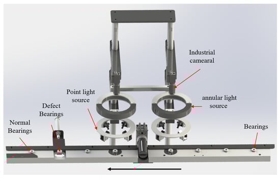
Figure 7. Bearing data collection platform.

The resolution of the collected images is 1280 × 1024, and the collected images are shown in Figure 8a. After the EDCircle method [36], the bearing area is extracted, and the inner ring area of the bearing is removed, as shown in Figure 8b. Then, the resolution of Figure 8b is adjusted to 416 × 416. 1700 images of defective bearing samples are collected. The defects are labeled by the professional annotation software Labelme. The labeling results are recorded in the a.json file. After processing the a.json file, the results (as shown in Figure 5d) are recorded as a semi-fine label.

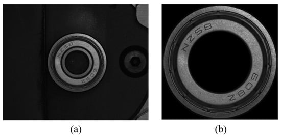
Figure 8. Data collected by the platform. (a) Original data (b) Bearing data.

The final data are shown in Table 3. Since the accuracy evaluation index is easily affected by sample imbalance, the number of defective data and non-defective data is kept consistent on the test dataset.

Table 3. Number of collected bearing datasets.

Type	Train	Valid	Test
Defect	960	240	500
Non-defect	2400	600	500

4.1.2. Magnetic-Tile Dataset

The Magnetic-Tile (MT) defect dataset [38] contains 392 defective images and 952 non-defective images. There are five types of defects in this dataset, which are blowhole, break, crack, fray, and uneven. Every image corresponds to a pixel-level label with different resolutions. We cut the image according to the center position of the label pixel and adjust the final resolution of the image to 192 × 192. Figure 9 shows some images and ground truth (GT) after processing.

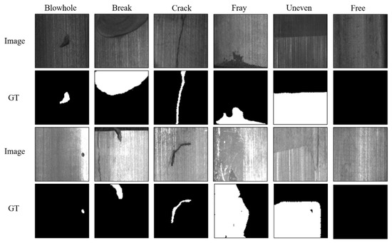
Figure 9. Examples of images from the MT defect dataset.

4.2. Implementation Details

The proposed PMG-Net is implemented in the PyTorch framework with an NVIDIA GTX2080TI (11G memory) on Ubuntu. The network optimizer is stochastic gradient descent (SGD) without momentum and weight decay. The learning rate is set to 0.01, the batch size is 16. And 80 training epochs are carried out. The weights are initialized to the convolutional blocks by the “Xavier” scheme. The training data and validation data are shown in Table 3. After many experiments, the weight label α is set to 2, and ω is set to 1 for Equation (7).

4.3. Performance Metrics

In all experiments, we focus on evaluating the classification metrics of every image, which are the most relevant metrics in industrial quality control, as they decide whether to keep or discard samples under inspection. Therefore, accuracy (ACC) and average precision (AP) are used to measure the classification performance of the PMG-Net. ACC is calculated by the ratio of all correctly detected samples to all samples in the dataset. The AP is calculated as the area under the curve of precision and recall. The recall rate R represents the ratio of samples with the positive test result to the actual positive samples in the test dataset. The higher the R is, the more positive samples are detected, and the missed detection rate is lesser. The ratio of the actual positive samples to the total number of positive samples detected is the precision rate P. The higher the P is, the lower the false detection rate is. Theoretically, higher P and R indicators are the ultimate aims of the detection, which is impossible in a practical situation. Considering P and R indicators comprehensively, F1 is introduced as the harmonic mean of P and R. The calculation of these indicators depends on the four parameters of sample classification as described follows:

$$ACC=\frac{TP+TN}{TP+TN+FP+FN}$$

(10)

$$P=\frac{TP}{TP+FP}$$

(11)

$$R=\frac{TP}{TP+FN}$$

(12)

$$AP={\int }_0^{1}P\left(R\right)dR$$

(13)

$$F1=\frac{2\ast P\ast R}{P+R}$$

(14)

where TP means true positive samples, which are positive samples and positively classified; FP means false positive, which are negative samples but positively classified; TN means true negative, which are negative samples and negatively classified. FN means false negative samples, which are positive samples but negatively classified.

4.4. Experiment Results and Analysis

To verify the superiority, robustness, and practicality of the PMG-Net, we designed the following experiments including comparison experiments with state-of-the-art methods, ablation experiments of the PMG-Net, and experiments on the MT defect dataset.

4.4.1. Methods Comparison

The performance of the proposed PMG-Net is firstly compared with other methods by training and testing the same data on our newly established dataset of bearing cover defects.

During the testing process, we regard samples with defects as positive samples and non-defective samples as negative samples. For the object detection network (Yolov6 and Yolov7), the threshold of intersection over union is set to 0.45, and the confidence is set to 0.25. For the classification of positive samples, the sample is classified as the correct positive sample if the object box contains a defect area; otherwise, it is classified as a wrong positive sample. For negative samples, it is considered a wrong negative sample if the object box is detected, and vice versa.

The performance comparison results of different methods are shown in Table 4 and Figure 10. Obviously, our PMG-Net is superior to other methods in AP value of bearing defect detection. Our method achieves a high ACC of 99.3%, which is increased by >2% compared with that of MixSeg (97.3%) and SegDecNet (97.0%). And there are only 7 recognition errors (0 + 7) of PMG-Net, which is fewer than that of MixSeg (27 (3 + 24) errors) and SegDecNet (30 (5 + 25) errors). Compared with Yolov6 and Yolov7, the ACC is increased by 3%~5%, and the number of recognition errors is reduced by 34 and 51, respectively. The FP of PMG-Net is 0, indicating that there is no false detection on the non-defect dataset. The FN is 7 and the missed detection rate is only 1.4%. Compared with other methods, PMG-Net has the lowest false detection rate and missed detection rate.

Table 4. The accuracy results of these five methods on the bearing dataset.

Method	AP	F1	ACC	FP + FN
MixSeg [37]	0.996	0.972	0.973	3 + 24
SegDecNet [39]	0.995	0.969	0.970	5 + 25
Yolov6 [40]	0.987	0.958	0.959	20 + 21
Yolov7 [41]	0.976	0.939	0.942	12 + 46
PMG-Net (ours)	0.999	0.993	0.993	0 + 7

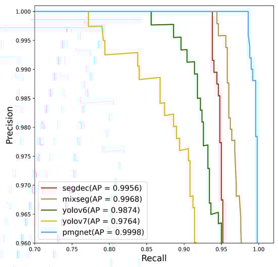
Figure 10. AP curve of different defect detection methods.

The detection results in a comparison of different methods are displayed in Figure 11. As shown in Figure 11b,c, the Yolov6 and Yolov7 have good recognition ability for small defects detection, but it is easily affected by materials and the change of font position. And they perform poorly in the recognition of large defects with low contrast, resulting in missed detections. The defects detection of MixSeg and SegDecNet (Figure 11d,e) are not affected by fonts and materials change, but small defects and large defects cannot be effectively identified at the same time. Our PMG-Net method achieves high recognition accuracy for defects of different sizes and non-defect data as shown in Figure 11f. Moreover, the defects detection results are insusceptible to the change of fonts and materials. The improved defects detection performance can be attributed to the following reasons: (1) The segmentation network is used to classify each pixel, so that the network can learn the detailed features of the same category and avoid the data inconsistency caused by materials. (2) The location of the segmentation result map is also relatively accurate, so as the prior knowledge, it can better guide the classification subnet to classify defects. (3) Through the multi-scale cross-fusion module, the network can make full use of context information, adapt to defect data of different scales, and enable the classification subnet to have a more accurate classification.

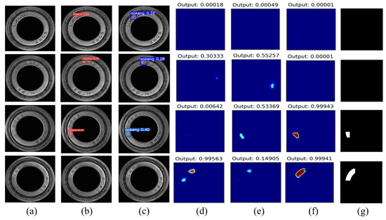
Figure 11. The result images of different methods. (a) Original image. (b) Yolov6. (c) Yolov7. (d) MixSeg. (e) SegDecNet. (f) PMG-Net. The first two rows are the data of non-defective bearings, and the last two rows are the data of defective bearings. (g) Ground truth.

4.4.2. Ablation Experiment

The PMG-Net mainly includes three modules in total, and to evaluate the function of every module, a series of ablation experiments including segmentation prior models (SegPM), PFFM, and weight label are performed in this part. The results of the ablation experiments are shown in Table 5.

Table 5. Performance of every individual module on the bearing dataset.

SegPM	PFFM	Weight Label	ACC	FP + FN
			0.853	75 + 72
√			0.949	21 + 30
√		√	0.965	10 + 25
√	√		0.972	18 + 10
√	√	√	0.993	0 + 7

SegPM: For the network only with the classification network (the SegPM, PFFM, and weight label are all removed), the ACC is 85.3% and there are 147(75 + 72) recognition errors. When the segmentation network is added as the prior model, the ACC improves to 94.9% on the bearing dataset and the number of recognition errors decreases to 51 (21 + 30). These results indicate that with the segmentation network as prior knowledge, the classification subnet can be better guided to classify samples. Meanwhile, the wrong features learned by the classification subnet can be corrected by the segmentation network.

Weight label: After introducing the weight label to the segmentation network, the ACC increased from 94.9% to 96.5% on the bearing dataset, which proves the effectiveness of the weight label. It can be seen from Figure 12 that when a weight label is added, the PMG-Net pays more attention to the central area of the pit defects and ignores some useless information in the edge area. That means the confidence of the center is high, and the confidence near the edge is small. In this way, the PMG-Net can avoid learning wrong features and increase the accuracy of identifying non-defective data.

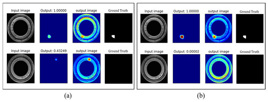
Figure 12. Comparison of weight label results. (a) Without weight label. (b) With weight label. The first row is defective data. The second row is non-defective data.

PFFM: When the PFFM module is added, the ACC increases from 94.9% to 97.2% on the bearing dataset without the introduction of a weight label. After the addition of the weight label, the ACC further increases from 97.2% to 99.3%. The results are shown in Figure 13. The addition of the PFFM module further improves the recognition accuracy of defect data. The segmentation network can combine global context information more efficiently, thus can recognize defects of various sizes and avoiding the information loss of small defects as the network deepens.

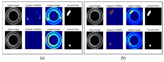
Figure 13. Comparison of PFFM results (with weight label). (a) Without PFFM. (b) With PFFM.

4.4.3. Robustness Experiment

To verify the robustness of the PMG-Net, we conducted experiments on the public MT dataset. The MT datasets have various defects, complex textures, and changeable light intensity. Due to the data imbalance of defect types in the MT dataset, the use of ACC as an evaluation metric will lead to data error. Therefore, AP is selected as an evaluation metric for the MT dataset. The results of various types of defects are shown in Table 6.

Table 6. The method is mentioned on the MT dataset with AP of different defects.

Type	Blowhole	Crack	Break	Fray	Uneven
AP	1.0	1.0	0.996	0.954	0.975

It can be seen from the table that our PMG-Net can reach the AP of 100% for the blowhole and crack-type defects. And the AP of the break and uneven type defects is 99.6% and 97.5%, respectively. The average AP value of the five types of defects is 98.5%. Figure 14 exhibits the output of PMG-Net operated on the MT dataset. Distinctly, our method has good adaptability to defects with different sizes, complex textures, and variational light.

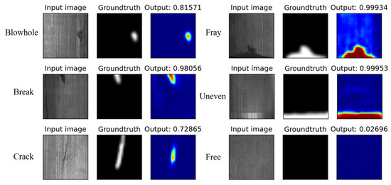
Figure 14. The output result images of the method mentioned on the MT dataset.

5. Conclusions

In this paper, we construct a dataset of 1700 images with annotation labels of defective bearing covers and 3500 images of non-defective bearing covers for the first time. And we also propose a PMG-Net for the pit defects detection on the bearing cover to realize fast quality inspection in the bearing production process. The PMG-Net is designed with a segmentation prior model, weight label, and pyramid cross-fusion module. The segmentation network can learn the detailed features of the same category through fine-grained segmentation. And as a prior model, it also can guide the classification network to classify. The introduction of weight labels can reduce the cost of the manual label. And the pyramid cross-fusion module is added to make the segmentation network fully obtain the context information, thus can detect defects of different sizes and avoiding the information loss of small defects, resulting in improved defects detection accuracy. The experimental results show that the PMG-Net can perfectly distinguish the defective and non-defective samples and shows high detection accuracy for the pit defects of different sizes on the bearing cover. And we also confirm the robustness of the PMG-Net on the public dataset. The PMG-Net still faces some challenges in recognizing some complicated samples, which all have very small defect areas and extremely low contrast. Therefore, in the future, we will dedicate our focus to the detection of weak and small defects on bearing covers.

References

- Liang, P.; Deng, C.; Wu, J.; Yang, Z.; Zhu, J. Intelligent fault diagnosis of rolling element bearing based on convolutional neural network and frequency spectrograms. In Proceedings of the 2019 IEEE International Conference on Prognostics and Health Management (ICPHM), San Francisco, CA, USA, 17–20 June 2019; pp. 1–5. [Google Scholar] [CrossRef]
- Volkau, I.; Mujeeb, A.; Dai, W.; Erdt, M.; Sourin, A. The Impact of a Number of Samples on Unsupervised Feature Extraction, Based on Deep Learning for Detection Defects in Printed Circuit Boards. Futur. Internet 2021, 14, 8. [Google Scholar] [CrossRef]
- Onchis, D.M.; Gillich, G.-R. Stable and explainable deep learning damage prediction for prismatic cantilever steel beam. Comput. Ind. 2020, 125, 103359. [Google Scholar] [CrossRef]
- Weimer, D.; Scholz-Reiter, B.; Shpitalni, M. Design of deep convolutional neural network architectures for au-tomated feature extraction in industrial inspection. CIRP Ann. 2016, 65, 417–420. [Google Scholar] [CrossRef]
- Yang, Y.; Yang, R.; Pan, L.; Ma, J.; Zhu, Y.; Diao, T.; Zhang, L. A lightweight deep learning algorithm for inspection of laser welding defects on safety vent of power battery. Comput. Ind. 2020, 123, 103306. [Google Scholar] [CrossRef]
- Yu, J.; Zheng, X.; Liu, J. Stacked convolutional sparse denoising auto-encoder for identification of defect patterns in semiconductor wafer map. Comput. Ind. 2019, 109, 121–133. [Google Scholar] [CrossRef]
- Lin, H.; Li, B.; Wang, X.; Shu, Y.; Niu, S. Automated defect inspection of LED chip using deep con-volutional neural network. J. Intell. Manuf. 2019, 30, 2525–2534. [Google Scholar] [CrossRef]
- Mahendran, A.; Vedaldi, A. Understanding deep image representations by inverting them. In Proceedings of the IEEE Conference on Computer Vision and Pattern Recognition, Boston, MA, USA, 7–12 June 2015; pp. 5188–5196. [Google Scholar]
- Long, J.; Shelhamer, E.; Darrell, T. Fully convolutional networks for semantic segmentation. In Proceedings of the IEEE Conference on Computer Vision and Pattern Recognition, Boston, MA, USA, 7–12 June 2015; pp. 3431–3440. [Google Scholar]
- Li, G.; Yu, Y. Visual saliency based on multiscale deep features. In Proceedings of the IEEE Conference on Computer Vision and Pattern Recognition, Boston, MA, USA, 7–12 June 2015; pp. 5455–5463. [Google Scholar]
- Zhao, R.; Ouyang, W.; Li, H.; Wang, X. Saliency detection by multi-context deep learning. In Proceedings of the IEEE Conference on Computer Vision and Pattern Recognition, Boston, MA, USA, 7–12 June 2015; pp. 1265–1274. [Google Scholar]
- Deng, C.; Wang, M.; Liu, L.; Liu, Y.; Jiang, Y. Extended Feature Pyramid Network for Small Object Detection. IEEE Trans. Multimedia 2021, 24, 1968–1979. [Google Scholar] [CrossRef]
- Lin, T.-Y.; Dollár, P.; Girshick, R.; He, K.; Hariharan, B.; Belongie, S. Feature pyramid networks for object detection. In Proceedings of the IEEE Conference on Computer Vision and Pattern Recognition, Honolulu, HI, USA, 21–26 July 2017. [Google Scholar]
- Lin, T.-Y.; Goyal, P.; Girshick, R.; He, K.; Dollár, P. Focal loss for dense object detection. In Proceedings of the IEEE International Conference on Computer Vision, Venice, Italy, 22–29 October 2017. [Google Scholar]
- Dong, H.; Song, K.; He, Y.; Xu, J.; Yan, Y.; Meng, Q. PGA-Net: Pyramid Feature Fusion and Global Context Attention Network for Automated Surface Defect Detection. IEEE Trans. Ind. Informatics 2019, 16, 7448–7458. [Google Scholar] [CrossRef]
- Liu, B.; Yang, Y.; Wang, S.; Bai, Y.; Yang, Y.; Zhang, J. An automatic system for bearing surface tiny defect detection based on multi-angle illuminations. Optik 2020, 208, 164517. [Google Scholar] [CrossRef]
- Shen, H.; Li, S.; Gu, D.; Chang, H. Bearing defect inspection based on machine vision. Measurement 2012, 45, 719–733. [Google Scholar] [CrossRef]
- Van, M.; Kang, H.-J. Wavelet Kernel Local Fisher Discriminant Analysis With Particle Swarm Optimization Algorithm for Bearing Defect Classification. IEEE Trans. Instrum. Meas. 2015, 64, 3588–3600. [Google Scholar] [CrossRef]
- Pacas, M. Sensorless harmonic speed control and detection of bearing faults in repetitive mechanical systems. In Proceedings of the 2017 IEEE 3rd International Future Energy Electronics Conference and ECCE Asia (IFEEC 2017-ECCE Asia), Kaohsiung, Taiwan, 3–7 June 2017; pp. 1646–1651. [Google Scholar]
- Chen, S.-H.; Perng, D.-B. Automatic Surface Inspection for Directional Textures Using Discrete Cosine Transform. In Proceedings of the THE 2009 Chinese Conference on Pattern Recognition, Nanjing, China, 4–6 November 2009; pp. 1–5. [Google Scholar] [CrossRef]
- Huang, Y.; Qiu, C.; Wang, X.; Wang, S.; Yuan, K. A Compact Convolutional Neural Network for Surface Defect Inspection. Sensors 2020, 20, 1974. [Google Scholar] [CrossRef]
- Kim, S.; Kim, W.; Noh, Y.-K.; Park, F. Transfer learning for automated optical inspection. In Proceedings of the 2017 International Joint Conference on Neural Networks (IJCNN), Anchorage, AK, USA, 14–19 May 2017; pp. 2517–2524. [Google Scholar]
- Lin, Z.; Ye, H.; Zhan, B.; Huang, X. An Efficient Network for Surface Defect Detection. Appl. Sci. 2020, 10, 6085. [Google Scholar] [CrossRef]
- Wang, T.; Chen, Y.; Qiao, M.; Snoussi, H. A fast and robust convolutional neural network-based defect detection model in product quality control. Int. J. Adv. Manuf. Technol. 2017, 94, 3465–3471. [Google Scholar] [CrossRef]
- Haselmann, M.; Gruber, D.; Tabatabai, P. Anomaly detection using deep learning based image completion. In Proceedings of the 2018 17th IEEE International Conference on Machine Learning and Applications (ICMLA), Orlando, FL, USA, 17–20 December 2018; pp. 1237–1242. [Google Scholar]
- Youkachen, S.; Ruchanurucks, M.; Phatrapomnant, T.; Kaneko, H. Defect Segmentation of Hot-rolled Steel Strip Surface by using Convolutional Auto-Encoder and Conventional Image processing. In Proceedings of the 2019 10th International Conference of Information and Communication Technology for Embedded Systems (IC-ICTES), Bangkok, Thailand, 25–27 March 2019; pp. 1–5. [Google Scholar] [CrossRef]
- Zhai, W.; Zhu, J.; Cao, Y.; Wang, Z. A Generative Adversarial Network Based Framework for Unsupervised Visual Surface Inspection. In Proceedings of the 2018 IEEE International Conference on Acoustics, Speech and Signal Processing (ICASSP), Calgary, AB, Canada, 15–20 April 2018; pp. 1283–1287. [Google Scholar] [CrossRef]
- Roth, K.; Pemula, L.; Zepeda, J.; Schölkopf, B.; Brox, T.; Gehler, P. Towards total recall in in-dustrial anomaly detection. In Proceedings of the IEEE/CVF Conference on Computer Vision and Pattern Recognition, New Orleans, LA, USA, 19–24 June 2022; pp. 14318–14328. [Google Scholar]
- Defard, T.; Setkov, A.; Loesch, A.; Audigier, R. PaDiM: A Patch Distribution Modeling Framework for Anomaly Detection and Localization. In Proceedings of the Pattern Recognition. ICPR International Workshops and Challenges, Virtual Event, 10–15 January 2021; LNCS Volume 12664, pp. 475–489. [Google Scholar] [CrossRef]
- Gudovskiy, D.; Ishizaka, S.; Kozuka, K. CFLOW-AD: Real-Time Unsupervised Anomaly Detection with Localization via Conditional Normalizing Flows. In Proceedings of the 2022 IEEE/CVF Winter Conference on Applications of Computer Vision (WACV), Waikoloa, HI, USA, 3–8 January 2022; pp. 1819–1828. [Google Scholar] [CrossRef]
- Yang, D.; Cui, Y.; Yu, Z.; Yuan, H. Deep Learning Based Steel Pipe Weld Defect Detection. Appl. Artif. Intell. 2021, 35, 1237–1249. [Google Scholar] [CrossRef]
- Cha, Y.J.; Choi, W.; Suh, G.; Mahmoudkhani, S.; Büyüköztürk, O. Autonomous structural visual in-spection using region-based deep learning for detecting multiple damage types. Comput. Aided Civ. Infrastruct. Eng. 2018, 33, 731–747. [Google Scholar] [CrossRef]
- Zhong, J.; Liu, Z.; Han, Z.; Han, Y.; Zhang, W. A CNN-Based Defect Inspection Method for Catenary Split Pins in High-Speed Railway. IEEE Trans. Instrum. Meas. 2018, 68, 2849–2860. [Google Scholar] [CrossRef]
- Zheng, Z.; Zhao, J.; Li, Y. Research on Detecting Bearing-Cover Defects Based on Improved YOLOv3. IEEE Access 2021, 9, 10304–10315. [Google Scholar] [CrossRef]
- Khan, A.; Chefranov, A.; Demirel, H. Image scene geometry recognition using low-level features fusion at multi-layer deep CNN. Neurocomputing 2021, 440, 111–126. [Google Scholar] [CrossRef]
- Akinlar, C.; Topal, C. EDCircles: A real-time circle detector with a false detection control. Pattern Recognit. 2012, 46, 725–740. [Google Scholar] [CrossRef]
- Božič, J.; Tabernik, D.; Skočaj, D. Mixed supervision for surface-defect detection: From weakly to fully supervised learning. Comput. Ind. 2021, 129, 103459. [Google Scholar] [CrossRef]
- Huang, Y.; Qiu, C.; Yuan, K. Surface defect saliency of magnetic tile. Vis. Comput. 2018, 36, 85–96. [Google Scholar] [CrossRef]
- Tabernik, D.; Šela, S.; Skvarč, J.; Skočaj, D. Segmentation-based deep-learning approach for surface-defect detection. J. Intell. Manuf. 2020, 31, 759–776. [Google Scholar] [CrossRef]
- Li, C.; Li, L.; Jiang, H.; Weng, K.; Geng, Y.; Li, L.; Ke, Z.; Li, Q.; Cheng, M.; Nie, W. YOLOv6: A single-stage object detection framework for industrial applications. arXiv 2022, arXiv:2209.02976. [Google Scholar]
- Wang, C.-Y.; Bochkovskiy, A.; Liao, H.-Y.M. YOLOv7: Trainable bag-of-freebies sets new state-of-the-art for real-time object detectors. arXiv 2022, arXiv:2207.02696. [Google Scholar]
Disclaimer/Publisher’s Note: The statements, opinions and data contained in all publications are solely those of the individual author(s) and contributor(s) and not of MDPI and/or the editor(s). MDPI and/or the editor(s) disclaim responsibility for any injury to people or property resulting from any ideas, methods, instructions or products referred to in the content. |
© 2023 by the authors. Licensee MDPI, Basel, Switzerland. This article is an open access article distributed under the terms and conditions of the Creative Commons Attribution (CC BY) license (https://creativecommons.org/licenses/by/4.0/).