Segmentation of Nucleus and Cytoplasm from H&E-Stained Follicular Lymphoma

Abstract

This paper proposes a noble image segment technique to differentiate between large malignant cells called centroblasts vs. centrocytes. A new approach is introduced, which will provide additional input to an oncologist to ease the prognosis. Firstly, a H&E-stained image is projected onto L*a*b* color space to quantify the visual differences. Secondly, this transformed image is segmented with the help of k-means clustering into its three cytological components (i.e., nuclei, cytoplasm, and extracellular), followed by pre-processing techniques in the third step, where adaptive thresholding and the area filling function are applied to give them proper shape for further analysis. Finally, the demarcation process is applied to pre-processed nuclei based on the local fitting criterion function for image intensity in the neighborhood of each point. Integration of these local neighborhood centers leads us to define the global criterion of image segmentation. Unlike active contour models, this technique is independent of initialization. This paper achieved 92% sensitivity and 88.9% specificity in comparing manual vs. automated segmentation.

1. Introduction

Cancer is a group of diseases that involve the uncontrollable development of aberrant cells that have the potential to spread to other body organs. One of many cancer categories, lymphomas represent a type that begins in white blood cells known as lymphocytes. These lymphomas are categorized into two groups. The first is Hodgkin’s lymphoma (HL), which affects the lymphatic system of the immune system, which fights infection. HL is characterized by an overgrowth of white blood cells called lymphocytes, leading to enlarged, mostly painless lymph nodes and growths throughout the body. The presence of REED-STERNBERG cells is confirmed by HL (abnormal lymphocytes that may contain more than one nucleus). Non-Hodgkins lymphoma (NHL) is the second classification, in which lymphocytes can grow into tumors (growths) all over the body without damaging the lymphatic system. REED-STERNBERG is absent from NHL. Since it is hard to research and analyze every type of cancer under one heading, this work focuses on follicular lymphoma, the most prevalent subtype of NHL [1,2,3,4].

1.1. An introduction to Follicular Lymphoma: A Subtype of NHL

FL is the most common in the NHL category. It is a slow-growing solid cancer across the world. FL is a lymphoid system cancer, a type of white blood cell (WBC) caused by the uncharacteristic growth of lymphocytes.

Clinical trials in the India and US [4,5] found that 1.8 million people have cancer in the US and 2.6 million in India. NHL represents 4.3% of all new cancer cases, i.e., 0.19 million people in 2021. Figure 1 suggests that, among all the non-Hodgkins lymphoma, 22% of the patients come under the FL category, i.e., approximately 43,214 people will suffer from FL in 2021 in the US and India. India’s number of cancer patients is expected to rise from 26.7 million in 2021 to 29.8 million in 2025. The Northeast and the North had the greatest incidence last year (2408 cases per 0.1 million) and (2177 per 0.1 million), respectively. Men presented a greater rate of diagnosis [4,5,6].

Figure 1. Classification of Non-Hodgkin Lymphoma: A Subtypes (Source: American Cancer Society).

1.2. Histopathological Analysis of Follicular Lymphoma

Histopathology refers to the microscopic examination of tissue to study the appearance of the disease. As in most types of cancer, histopathological analysis is vital to characterize the tumor histology for further treatment planning [1,2,3,4,7,8].

The FL prognosis has been conducted manually by visually examining tissue samples collected from patient biopsy [7,8,9,10,11,12]. Under a microscope, FL is frequently composed primarily of small cells called centrocytes and a few bigger centroblasts. Below are a few criteria that are noted while manually inspecting FL tissue.

• Centrocytes typically have cleaved nuclei and appear with an abnormal, stretched shape
• Centroblasts are more giant cells that may have round (non-cleaved) or cleaved nuclei.
• The number of centroblasts per high-power field (HPF) may be counted and used to estimate the severity of the disease.
• CBs frequently have more open chromatin, giving the nucleus a lighter appearance; they can be counted to estimate how aggressive the disease is.

According to World Health Organization (WHO), CBs are manually counted, and the average CB per HPF $\left(0.159 {\mathrm{mm}}^2\right)$ are reported for further FL slide classification.

If the count of CBs is less than 6 (i.e., 0–5), then histology is the grade I. If this number ranges from 6 to 15 per HPF, then FL histology is classified into grade II. Otherwise (count is more than 15), FL histology is classified into grade III, as shown in Figure 2 [3,6,7].

Figure 2. WHO classification of Follicular histology.

Currently, the prognosis of FL is determined manually using visual inspection of tissue samples acquired from patient biopsy [7,8,13]. This visual grading is time-consuming and can lead to incorrect conclusions due to inter and intra-reader variability, different staining procedures, and highly inhomogeneous images. A computer-assisted segmentation procedure for digitized histology is required for disease prognostics, allowing oncologists to anticipate which patients are prone to disease, disease outcome, and survival prospects. Developing a grading system that can segment many objects, deal with overlapping nuclei, and provide a better supplementary architecture of the tissue sample is necessary. The nuclear architecture of these lymphomas is essential in classifying the disease into different categories [10,11,14,15]. So, in this paper, a four steps methodology is presented. In the first step, the H&E-stained image is projected onto L*a*b* color space. This space-transformed stained image is the human eye’s perceptual level and allows us to quantify the visual differences. In the second step, this transformed image is segmented with the help of k-means clustering into its three cytological components (i.e., nuclei, cytoplasm, and extracellular). In the third step, pre-processing techniques based on adaptive thresholding and area-filling function are applied to give them proper shape for further analysis. Finally, in the fourth step, the demarcation process is applied to pre-processed nuclei based on the local fitting criterion function for image intensity in a neighborhood of each point. Integration of these local neighborhood centers leads us to define the global criterion of image segmentation. Later, a comparative analysis is performed based on past research. In this paper, unlike the previous contour-based segmentation algorithm, the methodology is independent of the initialization.

The above-enumerated objectives have been accomplished using a well-elaborated experimental setup followed by a color-based image segmentation algorithm. In the proposed research work, 467 images (Whole slide and cellular level) are used for the experiment performed to meet the objectives. Seventy-seven distinguished researchers have already cited 216 images from the American Society of Haematology (ASH). The number of images considered for grades I, II, and III is 148, 145, and 174, respectively. All the segmentation features are drawn from H&E-Stained FL images using MATLAB R2020a software (version 2020a) with windows 11 Home Single Language (version 21H2) and 64-bit operating system, with AMD Ryzen 5 3500U processor.

The following is a breakdown of the paper’s structure: A review of segmentation techniques and their application to follicular histology is presented in Section 2. In Section 3, an overview of the proposed approach is presented, followed by a description of four different steps. In Section 4, the result of the proposed model is presented. In Section 5, a discussion and comparison with the previous research are discussed in detail, followed by a proof of robustness from initialization. Finally, a healthy mathematical dialogue is placed to verify the robustness of the proposed segmentation approaches. Section 6 brings the paper to a close and discusses the future scope.

2. Literature Review

Image segmentation is extracting an image’s region of interest (ROI). The ROI and real-world objects may be strongly correlated. Image analysis is vital since segmentation outcomes affect feature extraction and classification. The medical field uses segmentation to separate desirable biological entities from the background. A generic segmentation task includes separating background tissue, a tumor from different tissue types, or separating cellular components, e.g., nuclei from background tissue from histopathological images. Table 1 highlights various segmentation approaches widely accepted and previously deployed in the case of follicular histology.

Table 1. Systematic review for segmenting FL histology.

Reference	Year of Publication	Dataset Used	Region of Interest	Segmentation Approaches
[16]	2007	Training Set: 3627 Testing Set: 1813 FL images	Isolation of follicular regions	Mean brightness value as a thresholding technique
[17]	2008	17 Whole slide FL image	CB and non-CB cells classification	Thresholding to isolate RBC and background followed by K-means clustering
[18]	2008	30 IHC Stained Images & 11 H&E-Stained FL images	From IHC-Stained- Follicular region and H&E-Stained centroblast	For detecting follicular region GLCM with S channel from HSV colour model and for CB detection extracted features reduced by PCA and allocation of K-means
[19]	2008	18 cases of MCL, 20 cases of CCL, and 9 FL	Overlapping cell nuclei	Last2edges algorithm followed by gradient vector flow algorithm to identify contours. Application of canny edge detector.
[20]	2009	17 whole slide images of FL	Isolation of Centroblasts	Thresholding, along with applications of K-means
[9]	2010	100 ROI of FL sample	Isolation of Centroblasts	Gaussian mixer model parameterized with expectation maximization.
[21]	2010	100 ROI of FL sample	Isolation of Centroblasts	Applications of mean shift elimination technique
[22]	2010	40 IHC stained FL images	Follicular region	Active contour Model
[23]	2011	15 IHC stained FL images	Follicular region	Region-based image segmentation using curve evolution techniques.
[24]	2011	10 FL images	Cellular nuclei	Thresholding followed by local Fourier transformation and application of K-means and KNN
[25]	2012	17 FL images	Identification of centroblast	k-means of clustering
[10]	2012	12 IHC and H&E- stained FL images	Follicular region	Otsu thresholding and intersection between R plane and B plane binary mask
[26]	2013	110 FL images	Follicular region	Application of contour algorithms
[27]	2014	12 FL images	Identification of centroblast	Otsu thresholding and LDA to segments nuclei followed by thresholding technique to remove RBCs
[28]	2014	300 cells of FL	Centroblast identification	Otsu thresholding
[29]	2014	20 FL slide stained with CD20 and H&E	Cytoplasmic element classification	Segmentation by touching cell splitting using GMM classification by the neuro-fuzzy inference system
[30]	2016	28 images of FL stained with PAX5 and H&E	Centroblast	k-means clustering and graph cut segmentation procedure
[31]	2017	H&E-Stained image	Segmentation of CD3+ & CD3-T cells	Entropy-based histogram thresholding
[32]	2019	H&E-Stained image	Differentiate between FL and follicular hyperplasia	Deep learning-based feature extraction
[33]	2020	H&E-Stained image	Differentiate between FL and follicular hyperplasia	CNN-based segmentation approaches
[34]	2020	H&E-Stained image	Differentiate between FL and follicular hyperplasia	Deep learning-based feature extraction

Various segmentation methodologies have been proposed to extract these quality parameters and keep visual differences based on textural heterogeneity [15,35,36,37] and the morphological structure [10,20,27] of each cytological component (nuclei, cytoplasm, extracellular component, RBC, and background). These morphological and textural parameters are extracted with various segmentation approaches, e.g., thresholding technique [16], Otsu thresholding [10,28], Otsu thresholding followed by LDA [27], thresholding followed by k-means [17,20,24,25], k-means with graph cut method [30], textural parameter followed by PCA and k-means [18], L2E along with canny edge and Hough transformation [19,38,39,40,41], gaussian mixer model and expectation maximization [9], mean shift elimination [21], contour models [21,23,42,43,44,45,46,47,48,49], color-coded map based [29], watershed [37,50], piecewise [51] entropy-based histogram [31], level-set [52], and transfer learning approaches for feature extraction [32,33,34] have been introduced to segment histopathological images. Many works have been performed in image segmentation, available in survey resources. However, there is still no universally accepted algorithm to segment the images as it is influenced by many aspects, such as the image’s texture, image content, and the inhomogeneity of images. In the next section, this paper proposes a noble approach to isolate various cytological components from H&E-stained FL tissue samples.

3. Proposed Methodology

Unsupervised segmentation divides the images into distinct cytological components to collect these data. Normally, there are five main components in H&E-stained FL images: the nucleus, cytoplasm, background, red blood cells, and extracellular material. The entire methodology is divided into four major steps. In the first step, H&E-stain is projected over L*a*b* color space, and then k-means clustering is used to isolate different cytological components in the second step. In the third step, pre-processing techniques of adaptive thresholding and area filling function are applied to give them proper shape. Finally, proper demarcation of each nucleus is performed. Figure 3 shows the flow of the proposed methodology to isolate different cytological components.

Figure 3. Process flow diagram of proposed segmentation approaches.

3.1. Projection of H&E-Stained Image over L*a*b* Color Space

Firstly, each of these components is expressed as a different color. Since the difference between two colors in the L*a*b* color space is perceptually uniform, the Euclidean distance can be employed as a measurement during the segmentation process. As a result of their relatively consistent patterns, RBCs and background regions can be distinguished by thresholding the intensity values in the RGB color space. RBCs and background are not comparatively useful when classifying FL histology, so our concentration is on identifying the rest cytological components. The remaining structures must divide into three clusters representing nuclei, cytoplasm, and extracellular material. The flow diagram to isolate different cytological components is explained in Figure 4. The image is projected onto this paper’s a*b*, L*a*, and L*b* spatial domains. Results for step 1 are placed in Section 4.1.

Figure 4. Process flow to isolate different cytological components from H&E-Stained image.

The L*a*b* (CIELab) space comprises three layers: the brightness layer L* and the chromaticity layers a* and b*, which show where the color falls along the red-green and blue-yellow axes, respectively. The converting formula first determines the tri-stimulus coefficients as follows:

$$\begin{gathered} X=0.4303R+0.3416G+0.1784B \\ Y=0.2219R+0.7068G+0.0713B \\ Z=0.0202R+0.1296G+0.9393B \end{gathered}$$

(1)

The calculation of the CIELab color model is as follows;

$$\begin{gathered} L^{*}=116\left\{h\left(\frac{Y}{Y_s}\right)\right\}-16 \\ {a}^{*}=500\left\{h\left(\frac{X}{X_s}\right)\right\}-h\left(\frac{Y}{Y_s}\right) \\ {b}^{*}=200\left\{h\left(\frac{Y}{Y_s}\right)\right\}-h\left(\frac{Z}{Z_s}\right) \end{gathered}$$

(2)

where the usual stimulus coefficients are $X_s, Y_s, \mathrm{and} Z_s$. In the next step, images extracted from L*a*b* spaces are fed into a k-means clustering algorithm.

3.2. K-Means Clustering Based Segmentation

Any image is divided into k groups using the popular k-means clustering algorithm. The process of clustering involves putting data points with similar feature vectors together in one cluster and putting data points with diverse feature vectors into other clusters. Let feature vector derived from $c$ clustered data be $D=\left\{d_i\right|i=1, 2, 3\dots \dots ,c\}$. The generalized algorithm initiates $k$ cluster centroids $C=\left\{c_j\right|j=1, 2, 3\dots .k\}$ by randomly selecting $k$ features vector form $C$. The feature vectors are then divided into k clusters using a chosen measure for distance, such as the Euclidean distance (Equation (3)), so that

$$E_{dis}=\left|\left|d_i-c_j\right|\right|$$

(3)

The feature vectors are then regrouped using the newly computed cluster centroids, originally calculated based on the group members. The clustering process ends when all cluster centroids begin toward convergence.

K-mean clustering helps to isolate nuclei (with blue), cytoplasm (cyan), and extracellular material (in yellow color) using the Euclidean distance matrix obtained from L*a*b* color space.

Choose $3$ cluster centres to coincide with k randomly chosen patterns inside the hypervolume containing the patterns set (C). Steps to implement k-means are defined below;

1-

Assign each pattern to the closest cluster center, i.e., $C_i, i=1, 2, 3$.

2-

Recompute the cluster centers using cluster memberships. $\left(\mathit{U}\right)$

$${\mathit{U}}_{i, j}=\{\begin{array}{c}1, {\left|\left|x_i-C_i\right|\right|}^2\le {\left|\left|x_j-C_k\right|\right|}^2, for each k\ne i\\ 0, otherwise\end{array}$$

3-

If convergence criteria are not met, go to step 2 with new cluster centers by the following equation, i.e.,

$$C_i=\frac{i}{G_i}{\displaystyle \sum }_{k, x_kϵG_i}{X}_k$$

$\mathrm{where}$ |$G_i$| is the size and the value of $\left|G_i\right|={\displaystyle \sum }_{j=1}^n{\mathit{U}}_{i.j}$.

Then, these clustered cytological components pass from the adaptive thresholding and filling function to provide the proper shape of the segmented region of interest.

3.3. Adaptive and Thresholding Function

Adaptive thresholding and filling functions are applied to smooth the isolated objects. It separates a segmented image into fractional regions or fractional images. It then determines two threshold values for each fractional image, resulting in varying adaptive threshold values, followed by the bwareaopen applied to suppress small objects. Finally, in the last step, the procedure for the boundarization of each nucleus takes place.

3.4. Procedure for Boundarization of Each Nucleus

First, consider a segmented image of nuclei I as a function $I: \Omega \to R$ and represented through Equation (4):

$$I=I_{input}\left(x\right)\ast B_{bias}+N_{noise}\left(x\right)$$

(4)

Here, $I_{input}$ represents an actual inputted image, $B_{bias}$ is the biased field that will account for inhomogeneity in the image and $N_{noise}$ is a gaussian noise having zero mean value, and $x$ denotes pixel intensity $ϵ R.$ There are two minor assumptions about $B_{bias}$ and $I_{input}$ is as follows:

• Pixel intensity will remain constant next to the point as the assumption is a biased field $B_{bias}$ is slowly varying.
• The H&E-stained FL image ($I_{input})$ has approximately N separate regions ${\Omega }_1,{\Omega }_2\dots {\Omega }_n$ with constant values $C_1,C_2\dots C_n$ respectively. So, based on these assumptions and Equation (4), isolating the regions $\left\{{\Omega }_i|\begin{array}{c}n\\ i=1\end{array}\right\}$, having constant $\left\{C_i|\begin{array}{c}n\\ i=1\end{array}\right\}$ and the bias field ($B_{bias}$) for inputted FL histology.

All three parameters are identified and described below.

Special local energy is defined in the local area based on the intensity that necessitates locating the circular neighborhood in the premises of radius $r$ with the aid of Equation (4) and assumptions. Any other point in the premises of ${\Omega }_i$ say $x$ must meet the following constraint ${\phi }_y\cong \left\{x :x-y\le r\right\}$, with each point $y\in {\Omega }_i$ as the centre. With the help of this property, it is conclusive that slowly changing $B_{bias}$ ($y$), all $x$ values in the circular neighbourhood of ${\phi }_y$ have values that are near to $B_{bias}\left(y\right)$. With this, the intensity value $B_{bias}\left(x\right) \ast I_{input}\left(x\right)$ in the subregion (${\phi }_y$) is close to the constant $B_{bias}\left(y\right) \ast C_i$. With this piece of information, Equation (4) is written as Equation (5):

$$I=B_{bias}\left(y\right)\ast C_i+N_{noise}\left(x\right)$$

(5)

This has led us to formulate the necessary energy at the controllable scale. This energy helps us to classify inputted images into N clusters with centers $m_i\approx B_{bias}\left(y\right)\ast C_i, i=1,2,3\dots n$. Now local intensities are classified using the k-mean clustering technique, as well as a new term $K \left(y-x\right)$, which acts as a kernel. If $x\notin {\phi }_y$ is the value of $K\left(y-x\right)=0$, then this term should be inserted, i.e., points that do not fall under the premises of constraint ${\phi }_y\cong \left\{x: x-y\le r\right\}$ when building the cluster are excluded. This kernel is crucial in formulating local energy, as seen in Equation (6).

$$E_y={\displaystyle \sum }_{i=1}^n\underset{{\phi }_y}{{\displaystyle \int }}K\left(y-x\right){\left|I\left(x\right)-m_i\right|}^{2}dx$$

(6)

The choice of the kernel is very flexible. This paper uses a gaussian kernel as described in Equation (7),

$$k\left(x,y\right)=e^{-\frac{\left(x^2+y2\right)}{2\ast \sigma 2}}$$

(7)

where $\sigma$ is a scaling parameter, and the value of $\sigma$ is chosen as four by the hit and trial method. Until now, the discussion is on locally formulated energy that is not affected by cluster energy. Equation (8) shows how to integrate the $E_y term$ with respect to $d\left(y\right)$ to make this energy global.

$$E_{Final}={{\displaystyle \int }}^{}\left\{{\displaystyle \sum }_{i=1}^n\underset{{\phi }_y}{{\displaystyle \int }}K\left(y-x\right)\left|I\left(x\right)-m_i\right|2dx\right\}dy$$

(8)

Because the proposed energy is dispersed among the regions $\left\{{\Omega }_i|\begin{array}{c}n\\ i=1\end{array}\right\}$, finding an overall energy minimization solution becomes extremely tough. As a result, we split the above energy in terms of Chan-Vese’s [46] level set formulation in Equation (8) and rewrite Equation (8) as Equation (9);

$$E_{Final}={{\displaystyle \int }}^{}\{{\displaystyle \sum }_{i=1}^2\underset{{\phi }_y}{{\displaystyle \int }}\begin{array}{c}K\left(y-x\right){\left|I\left(x\right)-B\left(y\right)C_i\right|}^2\ast M_i\left(\Phi \left(x\right)\right) d\left(x\right) \} d\left(y\right)\end{array}$$

(9)

Here, $M_1\left(\Phi \right)=h\left(\Phi \right) \& M_2\left(\Phi \right)=1-h\left(\Phi \right)$ are two classification values of the function $M_i\left(\Phi \left(x\right)\right)$ for two-level set formulation. In terms of ($\Phi , C, B$), this $E_{Final}$ can be decreased. We can acquire image Segmentation given by $\Phi ,C,B$. by minimizing this energy. This is an iterative procedure that is accomplished by minimizing $E_{Final}$ with respect to $\Phi , C, \mathrm{and} b$ respectively.

A.

Minimizing energy with respect to $\Phi$

Using the steepest gradient decent method to reduce the energy term (in Equation (9)) while keeping C and B constant [44,53,54], Gateaux derivatives $\frac{\partial \left(E_{final}\right)}{\partial \left(\Phi \right)}$ of energy $E_{Final}$ are calculated using Equation (10);

$$\frac{\partial \left(\Phi \right)}{\partial \left(t\right)}=-\delta \left(\Phi \right)\left(e_1-e_2\right)+\upsilon .\delta \left(\Phi \right).div\left(\frac{\nabla \Phi }{\left|\nabla \Phi \right|}\right)+\mu .div\left(d_p\left(\left|\nabla \Phi \right|\right)\nabla \Phi \right)$$

(10)

where $e_1 \mathrm{and} e_2$ are described in Equation (11):

$$e_i={{\displaystyle \int }}^{}K\left(y-x\right){\left|I\left(x\right)-m_i\right|}^{2}d\left(y\right)$$

(11)

where div (.) is the divergence operator, $\nabla$ gradient operator, and $d_p$ is defined is as follows: $d_p\left(s\right)\triangleq \frac{p\prime \left(s\right)}{s}$.

Equation (10), as described above, is to be solved for demarking the nuclei. The first term in the equation $-\delta \left(\Phi \right)\left(e_1-e_2\right)$ is a data term because it is derived from data fitting energy; this term is responsible for driving spline towards the object boundary. The second term $\upsilon .\delta \left(\Phi \right). div\left(\frac{\nabla \Phi }{\left|\nabla \Phi \right|}\right)$ has a smoothing effect on the zero-level contours, which is necessary to maintain the regularity of the contour. This term also keeps a record of the arc length. The third term $\mu . div\left(d_p\left(\left|\nabla \Phi \right|\right)\nabla \Phi \right)$ is called a regularization term because it maintains the regularity of the spline.

B.

Minimizing energy with respect to $C$

While minimizing the constant, terms $C_{1 }\mathrm{and} C_2$ in $C$ are updated as follows, keeping $\Phi \& B$ constant as shown in Equation (12):

$$C_i=\frac{{{\displaystyle \int }}^{}\left(B\ast K\right)I{\upsilon }_{i}dy}{{{\displaystyle \int }}^{}\left(B2\ast K\right){\upsilon }_{i}dy}, \left(i=1,2, \dots , n\right)$$

(12)

where ${\upsilon }_i=M_i\left(\Phi \right)$ K is defined as a kernel in Equation (6), and the ∗ is a convolution function.

C.

Minimizing energy with respect to $B$

While $\Phi \mathrm{and} C$ are preserved as constants, the minimization of energy with respect to $B$ is as described in Equation (13):

$$B=\frac{\left(I.I_{input}^{\left(1\right)}\right)\ast K}{I_{input}^{\left(2\right)}\ast K}$$

(13)

where $I_{input}^{\left(1\right)}={\displaystyle \sum }_{i=1}^n{C}_i{\upsilon }_i$ and $I_{input}^{\left(2\right)}={\displaystyle \sum }_{i=1}^n{C}_{i}2{\upsilon }_i$. According to Equations (12) and (13), the value of constant $C=\left(c_1,c_2,c_3\dots c_n\right)$ and the representative biased field B is updated. This way, the energy is reduced, and the demarcated image is obtained. This demarcated image provides a different perceptive to the analysis of each cytological component of the image. In the next section, the obtained segmented image is discussed.

4. Results

This section presents the results of each step discussed in the previous section. Later, a comparative analysis is presented based on the segmentation results (Previous research vs. proposed methodology).

4.1. Result of Representation of FL Image on L*a*b* Color Space

Although CIELAB’s (L*a*b*) color axes are less consistent, they nevertheless remain effective for anticipating small color variations, and thus very useful for those images which have inhomogeneous intensities. Since the L*a*b* color space is a three-dimensional real number space, it supports an infinite number of color representations. The L*a*b* color space separates image luminosity and color. This color space makes it simpler to divide the regions according to hue, regardless of lightness. Additionally, the color space is more in line with how the human eye perceives the image’s various white, blue-purple, and pink portions.

Figure 5 converts the RGB image to CIE L*a*b* transformation using Equation (2). The three-dimensional CIELAB space covers the complete spectrum of human color vision.

Figure 5. CIE L*a*b* transformation from RGB image.

All necessary color information is included in both the $a^{*}$ and $b^{*}$ layers. To categorize the colors in the $a^{*}{b}^{*}$ space, different color-based segmentation approaches can be employed. In Figure 6, projections of alternative two coordinators are shown. In the first image, a combination of $a^{*}{b}^{*}$ is shown, in the next image a combination of $a^{*}{L}^{*}$, and in the last image of Figure 6, the combination of $L^{*}{b}^{*}$ is shown.

Figure 6. CIE L*a*b* transformation, combining two coordinates each time.

4.2. Result of k-Means Clustering Algorithm

This transformed image passes through the k-means clustering procedure. This clustering procedure extracts three major cytological components: one in all nuclei, another in the cytoplasm, and the last in the extracellular components. In Figure 7, images (a), (d), and (i) are the 3-input image randomly taken from the database belonging to grades I, II, and III, respectively. In images (b), (f), and (j) representation of different hue levels of each cytological element are represented. Isolation of only nuclei is presented in images(c), (g), and (k). These images are hued with dark blue, while images(d), (h), and (l) represent three different clustered images.

Figure 7. Output of L*a*b* projected k-means clustering (K = 3) algorithm. (a,e,i) Input Images (b,f,j) Different hue levels (c,g,k) Isolation of nuclei (d,h,l) Clustered Images.

In the next step, with the help of another critical parameter, the cytoplasm is extracted from the given input images, as shown in Figure 8. Images (a) and (d) are input images, (c) and (f) are the images of cytoplasm with different hues, and images (b) and (e) present the binarization of images (c) and (f) via the adaptive thresholding procedure. These morphological features vector is essential and will help pathologists to classify histology into respective grades.

Figure 8. Isolating cytoplasm from H&E-Stained image.

A region-based level set formulation is introduced to define the boundary of the extracted nuclei. The result of this method is displayed in the next step.

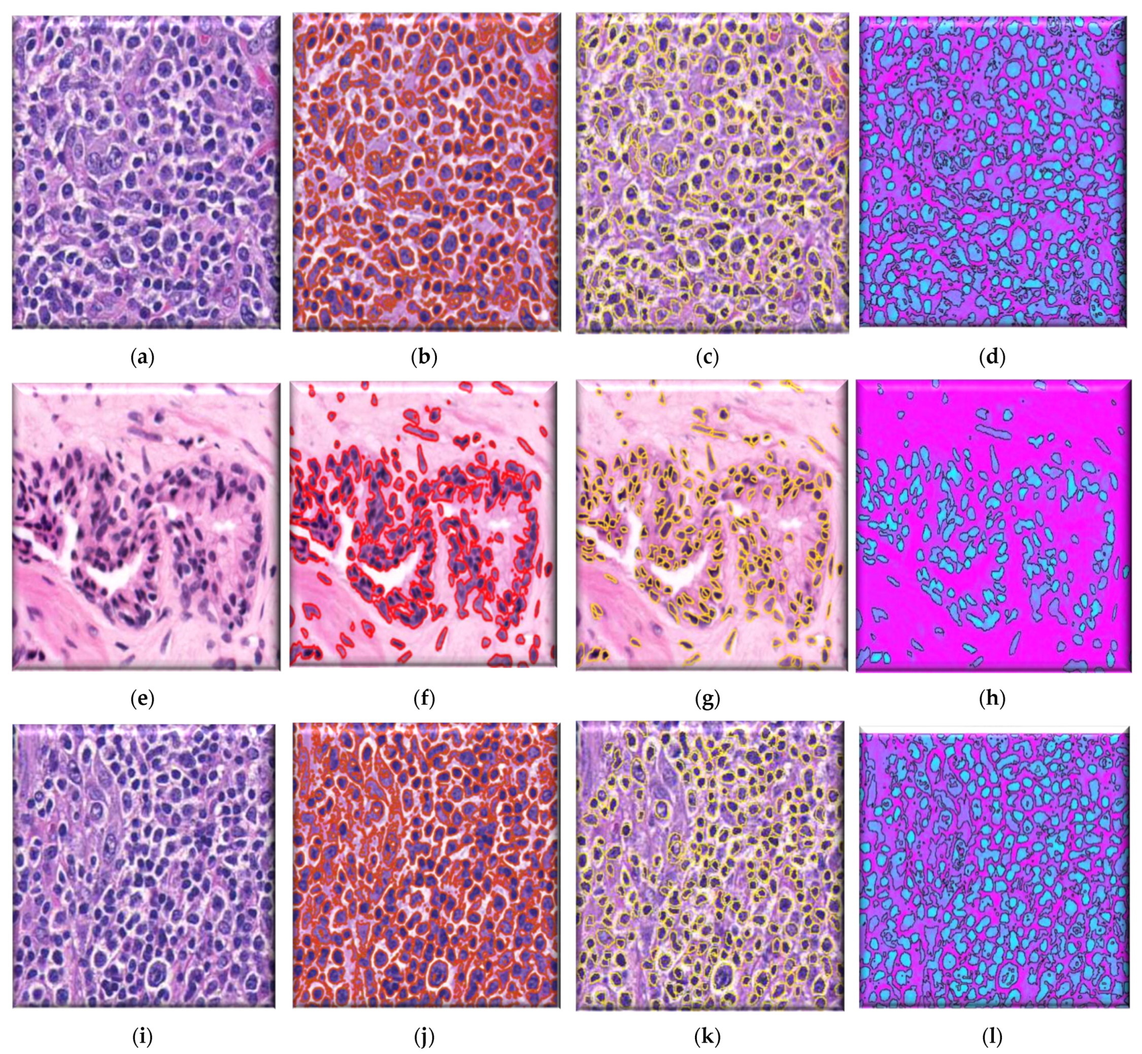
4.3. Procedure for Boundarization of Each Nucleus

This approach defines a local fitting criterion function for image intensity in a neighborhood of each point by assuming that pixel intensity will remain constant next to the point. Integration of these local neighborhood centers leads us to define the global criterion of image segmentation. To perform this experiment, values of certain parameters are described in Table 2. In Table 2, five different values of the coefficient of arc (1,0.5, 0.01, 0.001, and 0.0001) are chosen, and five different scale parameters (1, 2, 4, 6, 8). Table 2 shows the value of the coefficient of arc length can demark properly when the value is greater than 0.01, while the scale parameter starts showing better results when the value is exceeded by 4. So, in this paper, the coefficient of the arc length term is defined as $0.001\ast A^2$, where $A=255$, scale parameter that specifies the neighborhood size (σ = 4), outer iteration value is set to 100, which will keep track spline nearer to object, and the value of inner iteration is 20. Such inner iteration will help to level set evolution.

Table 2. Simulation of parameters.

Coefficient of Arc Length Term →	Scale Parameter →	1	0.5	0.01	0.001	0.0001
input image	1
	2
	4
	6
	8

The coefficient for distance regularization terms is set to 1. Experiment results are shown in Figure 9.

Figure 9. Demarcation with a red hue to each extracted nucleus.

In Figure 9, images (a), (d), and (g) are input images, and images (b), (e), and (h) are segmented images after the k-means clustering, thresholding function, and area-filling function. Images (c), (f), and (i) are the final images after the demarcation of each nucleus with red colour.

5. Discussion and Comparison with the Previous State of Arts

This paper comprises three images from the paper of A. Madabhushi et al. [44]. The GAC model, the method presented by A. Madabhushi et al. [44], and the suggested local energy formulation model are all compared qualitatively. Figure 10 shows the results for three images, demonstrating the model’s superiority in nucleus segmentation. We use the proposed model for segmenting the gland lumen and lymphocyte’s single white blood cell with a single round nucleus in the histopathological images used in this investigation. The nuclei segmentation results in Figure 10 exemplify the power of our local energy formulation model in detection, segmentation, and overlap resolution. Our local energy formulation model accurately segmented cells and cancer nuclei in histopathological images in Figure 10 (512 × 512 patches). Figure 10 highlights the model’s robustness by providing boundaries near the nuclear boundary and preventing spurious edges due to the form restriction. Compared to the GAC and the model by A. Madabhushi et al. [44], it also shows that our model can segment numerous overlapping objects. Table 3 explains the quantitative evaluation based on past research. In this table, the object of interest is either the classification between centroblast cells vs. non-centroblast cells or classifying different cytoplasmic elements. Some papers do not perform quantitative evaluation, while others applied a maximum of 90.35% accuracy while segmenting cytoplasmic elements. This paper proposed k-means-based, locally formulated energy to segment nuclei and cytoplasmic regions with 92% sensitivity.

Figure 10. (a,e,i) Original prostate histological image (b,f,j) Segmentation results from GAC Model (c,g,k) Segmentation results from Madabhushi’s model and (d,h,l) Results from proposed local energy formulation model.

Table 3. Quantitative evaluation of past research.

Ref.	Type of Staining & Dataset	Object of Interest	Evaluation Result
[16]	detection of follicles by IHC & classification of CB by H&E	classification between CB and non-CB cells	no performance evaluation is done
[18]	IHC stain for follicles detection followed by H&E stained for CB cells	classification between CB and non-CB cells	classification accuracy of 90.7%
[9]	H&E-Staining & 100 ROI images	CB & non-CB cells classification	Qualitative very high false-positive appealed
[21]	H&E-Staining100 ROI of FL images	CB & non-CB cells classification	Maximum accuracy of 80.7% achieved
[22]	436 images of Neoplastic Follicles	CB & non-CB cells classification	82.57% precision while segmenting
[25]	H&E Stained 17 FL images	Detection of nuclei and other cytological components	87% accuracy in classification
[27]	H&E Staining images 0f 180 FL samples	Centroblast detection	82.58% CB were successfully detected
[29]	H&E-Stained images	Cytoplasmic element classification	90.35% detection rate achieved
Proposed k-means based locally formulated energy	467 H&E-Stained Images	Extraction of Cytoplasmic element	92% sensitivity

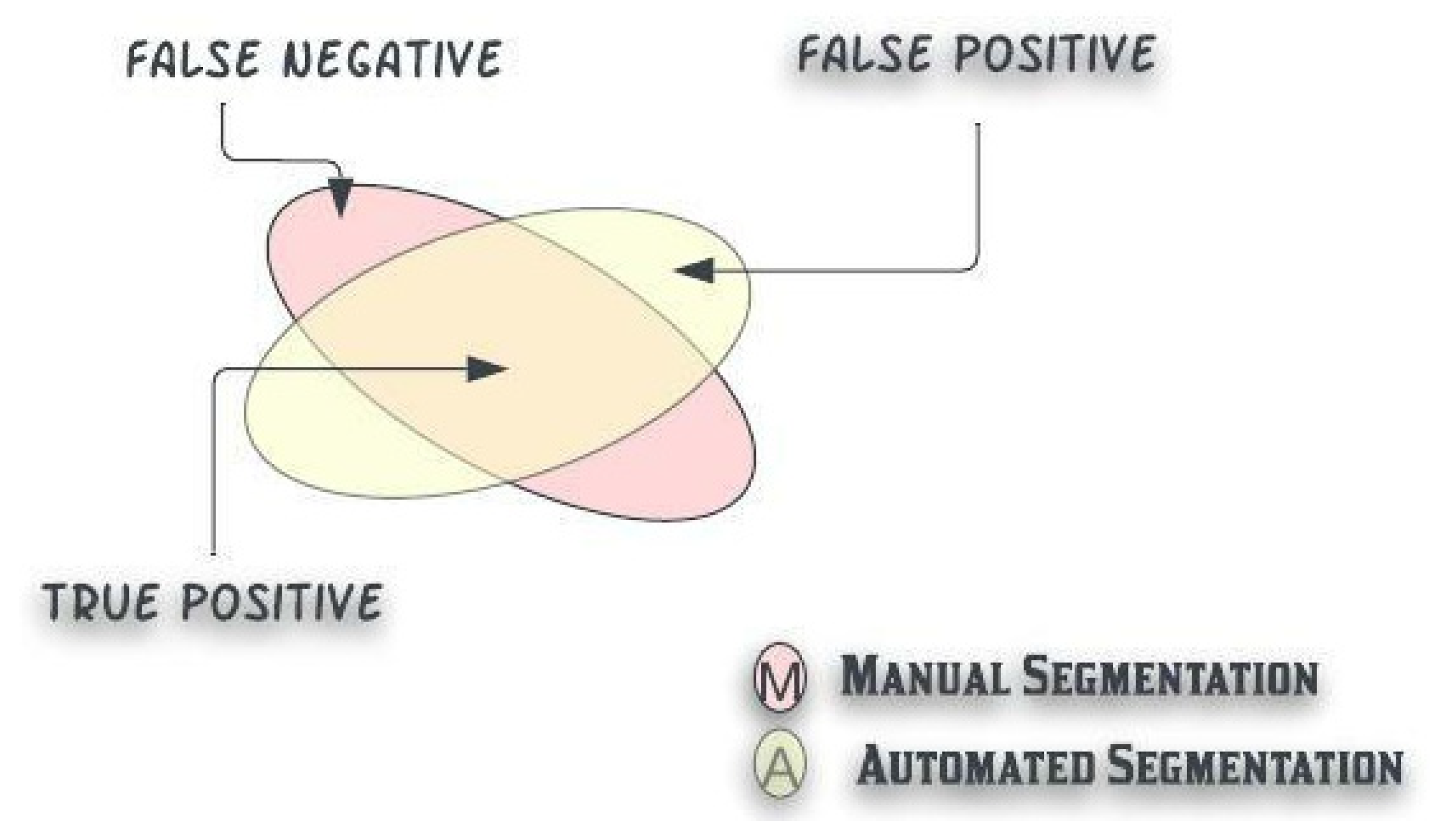
5.1. Quantitative Evaluation of the Proposed Segmentation Technique

The quantitative evaluation of the segmented nucleus and cytoplasm region is evaluated based on sensitivity, η, and specificity, δ.

In Figure 11, definitions of true positive (TP), true negative (TN), false positive (FP), and false negative are illustrated. The definition of sensitivity (η) and specificity (δ) is defined below:

$$\mathsf{\eta }=\frac{\mathrm{True} \mathrm{Positive}}{\mathrm{True} \mathrm{Positive}+\mathrm{False} \mathrm{Negative}}$$

(14)

$$\mathsf{\delta }=\frac{\mathrm{True} \mathrm{Negative}}{\mathrm{Ture} \mathrm{Negative}+\mathrm{False} \mathrm{Positive}}$$

(15)

Figure 11. Defining the evaluation standard: True negative, False Positive, True positive in automated vs. manual segmentation.

The quantitative evaluation of the proposed algorithm is conducted over 1283 nuclei extracted from 200 FL images and shown in Figure 12. The comparison is based on manual (graded data from pathology) vs. automated computerized segmentation techniques.

Figure 12. Image (a) is extracted region of interest by manual segmentation data set, image (b) is the outcome after proposed k-means clustering approaches, and image (c) is the outcome of the proposed algorithm.

Each ROI has been altered to be the same size as what pathologists would see in a high-power field of $0.159 {\mathrm{mm}}^2.$ In Table 4, a summarization of the detected outcome is placed. Based on TP, FP, FN, and TN, two classes of the given slide can be analyzed.

Table 4. Analysis of CB detection based on the proposed detection algorithm.

Name of Image	Manual Segmentation		Automated Segmentation
	Number of CBs	Number of Non-CBs	TP	FP	FN	TN
FL1	5	3	5	1	0	2
FL2	6	11	6	1	1	9
FL3	4	4	3	1	1	3
FL4	1	12	1	1	0	11
FL5	8	4	8	0	0	7

The two classes are displayed in Table 4. In the first column, input images are placed. The second column result of manual segmentation (number of centroblasts/number of non-centroblast) and the result of automated segmentation are placed in the last section. Table 5 describes the confusion matrix to elaborate on the accuracy of the proposed model based on two classes.

Table 5. Confusion matrix to elaborate accuracy of the proposed methodology.

	Centroblast	Non-Centroblast
Centroblast	True Positive	False Positive
Non-centroblast	False Negative	True Negative

This paper achieved a sensitivity (η) of 92% while the specificity (δ) is 88.9% recorded.

5.2. Independent from the Contour Initialization

Previously deployed region-based contour algorithms are dependent on the initialization of the contour [37,43,45,46,47,48,49], which implies that flowing energy goes downcast for those nuclei that are placed far from the initialization. Therefore, Section 4 explains the goal of creating an algorithm free from initialization. Initially, the first row displays the inputted image of follicular lymphoma. Four out of the twelve initializations of the contour are shown in Figure 13 for a qualitative evaluation of the system’s performance.

Figure 13. Follicular imagery, independent from contour initialization.

The second row displays four different locations of initialization over a biased region, and the third row contains an outline of the entire slide’s nucleus. The system achieves nearly the same result for the biased region and highlighted nucleus despite the substantial variation in contour initialization.

6. Conclusions and Future Scope

This study presents a new segmentation procedure for segmenting the different cytological components. The first step, the H&E-stained follicular histology image, is projected onto L*a*b* color space. This space-transformed stained image is the human eye’s perceptual level and allows us to quantify the visual differences. In the second step, this transformed image is segmented with the help of k-means clustering into its three cytological components. In the third step, pre-processing techniques based on adaptive thresholding and area-filling function are applied to give them proper shape for further analysis. Finally, in the fourth step, the demarcation process is applied to the pre-processed nucleus based on the local fitting criterion function for image intensity in the neighborhood of each point. This technique is independent of the initialization. This segmentation method employs a process known as local intensity fitting, which is utilized to recognize the unique shapes in the images precisely. This paper can achieve 92% sensitivity and 88.9% specificity to compare manual and automated segmentation.

Furthermore, the algorithm can distinguish between overlapped nuclei because object landmarks must be found across numerous objects for initial alignment. Thus, the relevant issue does not limit our model. The capacity to segregate lymphocytes in FL histopathological images automatically and accurately could be useful. This research does not classify follicular tissue. Rather, it divides it into cytological components. By separating all of the cytological components in the image, this method sets a new standard in digitalized histopathology. The algorithm analyses the complete tissue segment for diagnosing and grading the diseased, giving oncologists an additional representation to improve diagnostic accuracy at the outset. Furthermore, removing the need for initialization makes this approach more resilient and general.

References

1. Siegel, R.L.; Miller, K.D.; Jemal, A. Cancer Statistics. CA Cancer J. Clin. 2021, 71, 7–33. [Google Scholar] [CrossRef]
2. National Cancer Institute United State. Cancer Stat Facts: Non-Hodgkin Lymphoma. Available online: https://seer.cancer.gov/statfacts/html/nhl.html (accessed on 30 July 2021).
3. Teras, L.R.; DeSantis, C.E.; Cerhan, J.R.; Morton, L.M.; Jemal, A.; Flowers, C.R. 2016 US Lymphoid Malignancy Statistics by World Health Organization Subtypes. CA Cancer J. Clin. 2016, 66, 443–459. [Google Scholar] [CrossRef]
4. India Against Cancer; National Institute of Cancer Prevention and Research, Indian Council of Medical Research (ICMR). Available online: http://cancerindia.org.in/ (accessed on 30 July 2021).
5. Nair, R.; Arora, N.; Mallath, M.K. Epidemiology of Non-Hodgkin’s Lymphoma in India. Oncology 2016, 91, 18–25. [Google Scholar] [CrossRef]
6. Swerdlow, S.; Campo, E.; Harris, N.; Jaffe, E.; Pileri, S.; Stein, T.H.; Vardiman, J. WHO Classification of Tumors of Haematopoietic and Lymphoid Tissues, 4th ed.; World Health Organization: Lyon, France, 2008; Volume 2.
7. Hitz; Kettererb, F.; Lohric, A.; Meyd, U.; Pederivae, S.; Rennerf, C.; Tavernag, C.; Hartmannh, A.; Yeowi, K.; Bodisj, S.; et al. Diagnosis and treatment of follicular lymphoma European journal of medical sciences. Swiss Med. Wkly. 2011, 141, w13247. [Google Scholar]
8. Samsi, S.; Lozanski, G.; Shanarah, A.; Krishanmurthy, A.K.; Gurcan, M.N. Detection of Follicles from IHC Stained Slide of Follicular lymphoma Using Iterative Watershed. IEEE Trans. Biomed. Eng. 2010, 57, 2609–2612. [Google Scholar] [CrossRef] [Green Version]
9. Sertel, O.; Lozanski, G.; Shana’ah, A.; Gurcan, M.N. Computer-aided Detection of Centroblast for Follicular Lymphoma Grading using Adaptive Likelihood based Cell Segmentation. IEEE Trans. Biomed. Eng. 2010, 57, 2613–2616. [Google Scholar] [CrossRef] [Green Version]
10. Oztan, B.; Kong, H.; Metin; Gurcan, N.; Yener, B. Follicular Lymphoma Grading using cell-Graphs and Multi-Scale Feature Analysis. In Proceedings of the SPIE Medical Imaging, San Diego, CA, USA, 8–9 February 2012; Volume 83, pp. 345–353. [Google Scholar]
11. Gurcan, M.; Boucheron, L.; Can, A.; Madabhushi, A.; Rajpoot, N.; Yener, B. Histopathology Image Analysis: A Review. IEEE Rev. Biomed. Eng. 2009, 2, 147–171. [Google Scholar] [CrossRef] [Green Version]
12. Anneke, G.; Bouwer, B.; Imhoff, G.W.; Boonstra, R.; Haralambieva, E.; Berg, A.; Jong, B. Follicular Lymphoma grade 3B includes 3 cytogenetically defined subgroups with primary t(14;18), 3q27, or other translations: T(14;18) and 3q27 are mutually exclusive. Blood J. Hematol. Libr. 2013, 101, 1149–1154. [Google Scholar]
13. Mabadhushi, A.; Xu, J. Digital Pathology image analysis: Opportunities and challenges. Image Med. 2009, 1, 7–10. [Google Scholar] [CrossRef] [Green Version]
14. Mansoor, A.; Bagci, U.; Foster, B.; Xu, Z.; Papadakis, G.Z.; Folio, R.; Udupa, M.K.; Mollura, D.J. Segmentation and Image Analysis of Abnormal Lungs at CT: Current Approaches, Challenges, and Future Trends. Radiographics 2015, 35, 1056. [Google Scholar] [CrossRef] [Green Version]
15. Noor, N.; Than, J.; Rijal, O.; Kassim, R.; Yunus, A.; Zeki, A. Automatic Lung Segmentation Using Control Feedback System: Morphology and Texture Paradigm. J. Med. Syst. 2015, 39, 22. [Google Scholar] [CrossRef] [PubMed]
16. Zorman, M.; Kokol, P.; Lenic, M.; de la Rosa, J.L.S.; Sigut, J.F.; Alayon, S. Symbol-based machine learning approach for supervised segmentation of follicular lymphoma images. In Proceedings of the IEEE International Symposium on Computer-Based Medical Systems, Maribor, Slovenia, 20–22 June 2007; pp. 115–120. [Google Scholar]
17. Sertel, O.; Kong, J.; Lozanski, G.; Shana’ah, A.; Catalyurek, U.; Saltz, J.; Gurcan, M. Texture classification using nonlinear color quantization: Application to histopathological image analysis. In Proceedings of the IEEE International Conference on Acoustics, Speech and Signal Processing, Las Vegas, NV, USA, 31 March–4 April 2008; pp. 597–600. [Google Scholar]
18. Sertel, O.; Kong, J.; Lozanski, G.; Catalyurek, U.; Saltz, J.H.; Gurcan, M.N. Computerized microscopic image analysis of follicular lymphoma. In Proceedings of the Medical Imaging 2008: International Society for Optics and Photonics, San Diego, CA, USA, 17–19 February 2008; Volume 6915, p. 691535. [Google Scholar]
19. Yang, L.; Tuzel, O.; Meer, P.; Foran, D.J. Automatic image analysis of histopathology specimens using concave vertex graph. In Proceedings of the Medical Image Computing and Computer-Assisted Intervention, New York, NY, USA, 6–10 September 2008; Volume 11, pp. 833–841. [Google Scholar]
20. Sertel, O.; Kong, J.; Catalyurek, U.V.; Lozanski, G.; Saltz, J.H.; Gurcan, M.N. Histopathological image analysis using model-based intermediate representations and color texture: Follicular lymphoma grading. J. Signal Process. Syst. 2009, 55, 169–183. [Google Scholar] [CrossRef]
21. Sertel, O.; Catalyurek, U.V.; Lozanski, G.; Shanaah, A.; Gurcan, M.N. An image analysis approach for detecting malignant cells in digitized h&e-stained histology images 475 of follicular lymphoma. In Proceedings of the 20th IEEE International Conference on Pattern Recognition, Istanbul, Turkey, 23–26 August 2010; pp. 273–276. [Google Scholar]
22. Belkacem-Boussaid, K.; Prescott, J.; Lozanski, G.; Gurcan, M.N. Segmentation of follicular regions on H&E slides using a matching filter and active contour model. In Proceedings of the SPIE Medical Imaging, International Society for Optics and Photonics, San Diego, CA, USA, 13–18 February 2010; Volume 7624, p. 762436. [Google Scholar]
23. Belkacem-Boussaid, K.; Samsi, S.; Lozanski, G.; Gurcan, M.N. Automatic detection of follicular regions in H&E images using iterative shape index. Comput. Med. Imaging Graph. 2011, 35, 592–602. [Google Scholar] [PubMed] [Green Version]
24. Kong, H.; Belkacem-Boussaid, K.; Gurcan, M. Cell nuclei segmentation for histopathological image analysis. In Proceedings of the SPIE Medical Imaging: International Society for Optics and Photonics, San Francisco, CA, USA, 22–27 January 2011; p. 79622R. [Google Scholar]
25. Kong, H.; Gurcan, M.; Belkacem-Boussaid, K. Partitioning histopathological images: An integrated framework for supervised color-texture segmentation and cell 610 splitting. IEEE Trans. Med. Imaging 2011, 30, 1661–1677. [Google Scholar] [CrossRef] [Green Version]
26. Oger, M.; Belhomme, P.; Gurcan, M.N. A general framework for the segmentation of follicular lymphoma virtual slides. Comput. Med. Imaging Graph. 2012, 36, 442–451. [Google Scholar] [CrossRef] [PubMed] [Green Version]
27. Saxena, P.; Singh, S.K.; Agrawal, P. A heuristic approach for determining the shape of nuclei from H&E-stained imagery. In Proceedings of the IEEE Students Conference on Engineering and Systems, Allahabad, India, 12–14 April 2013; pp. 1–6. [Google Scholar]
28. Michail, E.; Kornaropoulos, E.N.; Dimitropoulos, K.; Grammalidis, N.; Koletsa, T.; Kostopoulos, I. Detection of centroblasts in H&E stained images of follicular lymphoma. In Proceedings of the Signal Processing and Communications Applications Conference, Trabzon, Turkey, 23–25 April 2014; pp. 2319–2322. [Google Scholar]
29. Dimitropoulos, K.; Michail, E.; Koletsa, T.; Kostopoulos, I.; Grammalidis, N. Using adaptive neuro-fuzzy inference systems for the detection of centroblasts in microscopic images of follicular lymphoma. Signal Image Video Process. 2014, 8, 33–40. [Google Scholar] [CrossRef]
30. Dimitropoulos, K.; Barmpoutis, P.; Koletsa, T.; Kostopoulos, I.; Grammalidis, N. Automated detection and classification of nuclei in pax5 and h&e-stained tissue sections of follicular lymphoma. Signal Image Video Process. 2016, 11, 145–153. [Google Scholar]
31. Abas, F.S.; Shana’ah, A.; Christian, B.; Hasserjian, R.; Louissaint, A.; Pennell, M.; Sahiner, B.; Chen, W.; Niazi, M.K.; Lozanski, G.; et al. Computer-assisted quantification of CD3+ T cells in follicular lymphoma. Cytom. Part A 2017, 91, 609–621. [Google Scholar] [CrossRef] [Green Version]
32. Syrykh, C.; Abreu, A.; Amara, N.; Siegfried, A.; Maisongrosse, V.; Frenois, F.X.; Martin, L.; Rossi, C.; Laurent, C.; Brousset, P. Accurate diagnosis of lymphoma on whole-slide histopathology images using deep learning. NPJ Digit. Med. 2020, 3, 63. [Google Scholar] [CrossRef]
33. Thiam, Y.; Vailhen, N.; Abreu, A.; Syrykh, C.; Frenois, F.; Ricci, R.; Tesson, B.; Sondaz, D.; Gomez, E.; Grivel, A.; et al. Artificial Intelligence Against Lymphoma: A New Deep Learning Based Anatomopathology Assistant to Distinguish Follicular Lymphoma from Follicular Hyperplasia. Eur. Hematol. Assoc. Libr. 2020, 298107, PB2193. [Google Scholar]
34. Brousset, P.; Syrykh, C.; Abreu, A.; Amara, N.; Laurent, C. Diagnosis and Classification Assistance from Lymphoma Microscopic Images Using Deep Learning. Hematol. Oncol. 2019, 37, 138. [Google Scholar] [CrossRef] [Green Version]
35. Yuan, J.; Wang, D.; Li, R. Remote sensing image segmentation by combining spectral and texture features. IEEE Trans. Geosci. Remote Sens. 2014, 52, 16–24. [Google Scholar] [CrossRef]
36. Reska, D.; Boldak, C.; Kretowski, M. A Texture-Based Energy for Active Contour Image Segmentation. In Image Processing & Communications Challenges 6; Springer: Cham, Switzerland, 2015; Volume 313, pp. 187–194. [Google Scholar]
37. Wenzhong, Y.; Xiaohui, F. A watershed-based segmentation method for overlapping chromosome images. In Proceedings of the 2nd International Workshop Education Technology Computer Science, Wuhan, China, 6–7 March 2010; Volume 1, pp. 571–573. [Google Scholar]
38. Leandro, A.; Fernandes, F.; Oliveira, M. Real-time line detection through an improved Hough transform voting scheme. Pattern Recognit. 2008, 41, 299–314. [Google Scholar]
39. Duda, R.; Hart, P. Use of the Hough Transformation to Detect Lines and Curves in Pictures. Graph. Image Process. 1972, 15, 11–15. [Google Scholar] [CrossRef]
40. O’Gorman, F.; Clowes, M. Finding picture edges through collinearity of feature points. IEEE Trans. Comput. 1976, 25, 449–456. [Google Scholar] [CrossRef]
41. Rizon, M.; Yazid, H.; Saad, P.; Shakaff, A.Y.; Saad, A.R.; Sugisaka, M.; Yaacob, S.; Mamat, M.; Karthigayan, M. Object Detection using Circular Hough Transform. Am. J. Appl. Sci. 2005, 2, 1606–1609. [Google Scholar] [CrossRef]
42. Fatakdawala, H.; Xu, J.; Basavanhally, A.; Bhanot, G.; Ganesan, S.; Feldman, M.; Tomaszewski, J.; Madabhushi, A. Expectation maximization driven geodesic active contour with overlap resolution (EMaGACOR): Application to lymphocyte segmentation on breast cancer histopathology. IEEE Trans. Biomed. Eng. 2010, 57, 1676–1689. [Google Scholar] [CrossRef]
43. Kass, M.; Witkin, A.; Terzopolos, D. Snakes: Active Contour Models. Int. J. Comput. Vis. 1998, 1, 321–331. [Google Scholar] [CrossRef]
44. Madabhushi, A.; Ali, S. An Integrated Region-, boundary-, Shape-Based Active Contour for Multiple Object Overlap Resolution in Histological Imagery. IEEE Trans. Med. Imaging 2012, 31, 1448–1460. [Google Scholar]
45. Vese, L.; Chan, T. A multiphase level set framework for image segmentation using the Mumford and Shah model. Int. J. Comput. Vis. 2002, 50, 271–293. [Google Scholar] [CrossRef]
46. Chan, T.; Vese, L. Active contours model without edges. IEEE Trans. Image Process. 2001, 10, 266–277. [Google Scholar] [CrossRef] [Green Version]
47. Caselles, V.; Kimmel, R.; Sapiro, G. Geodesic active contours. Int. J. Comput. Vis. 1997, 22, 61–79. [Google Scholar] [CrossRef]
48. Paragios, N.; Deriche, R. Geodesic active contours and level sets for detection and tracking of moving objects. IEEE Trans. Pattern Anal. Mach. Intell. 2000, 22, 266–280. [Google Scholar] [CrossRef] [Green Version]
49. Blake, A.; Isard, M. Active Contours; Springer Society: Cambridge, UK, 1998. [Google Scholar]
50. Mohammed, E.A.; Mohamed, M.M.A.; Naugler., C.; Far, B.H. Chronic lymphocytic leukemia cell segmentation from microscopic blood images using watershed algorithm and optimal thresholding. In Proceedings of the Annual IEEE Canadian Conference on Electrical and Computer Engineering, Regina, SK, Canada, 5–8 May 2013; pp. 1–5. [Google Scholar]
51. Mumford, D.; Shah, J. Optimal approximations by piecewise smooth functions and associated variational problems. Commun. Pure Appl. Math. 1989, 42, 577–685. [Google Scholar] [CrossRef]
52. Chan, T. Level Set Based Shape Prior Segmentation. In Proceedings of the IEEE Computer Society Conference Computation Vision Pattern Recognition, San Diego, CA, USA, 20–25 June 2005; Volume 2, pp. 1164–1170. [Google Scholar]
53. Aubert, G.; Kornprobst, P. Mathematical Problems in Image Processing; Partial Differential Equations and the Calculus of Variations; Springer: New York, NY, USA, 2002. [Google Scholar]
54. Evans, L. Partial Differential Equations; American Mathematics Society: Providence, RI, USA, 1998. [Google Scholar]