Hyperspectral Image Classification Using Geodesic Spatial–Spectral Collaborative Representation

Abstract

With the continuous advancement of remote sensing technology, the information encapsulated within hyperspectral images has become increasingly enriched. The effective and comprehensive utilization of spatial and spectral information to achieve the accurate classification of hyperspectral images presents a significant challenge in the domain of hyperspectral image processing. To address this, this paper introduces a novel approach to hyperspectral image classification based on geodesic spatial–spectral collaborative representation. It introduces geodesic distance to extract spectral neighboring information from hyperspectral images and concurrently employs Euclidean distance to extract spatial neighboring information. By integrating collaborative representation with spatial–spectral information, the model is constructed. The collaborative representation coefficients are obtained by solving the model to reconstruct the testing samples, leading to the classification results derived from the minimum reconstruction residuals. Finally, with comparative experiments conducted on three classical hyperspectral image datasets, the effectiveness of the proposed method is substantiated. On the Indian Pines dataset, the proposed algorithm achieved overall accuracy (OA) of 91.33%, average accuracy (AA) of 93.81%, and kappa coefficient (Kappa) of 90.13%. In the case of the Salinas dataset, OA was 95.62%; AA was 97.30%; and Kappa was 93.84%. Lastly, on the PaviaU dataset, OA stood at 95.77%; AA was 94.13%; and Kappa was 94.38%.

1. Introduction

Remote sensing technology, first proposed by American scientist Pruitt in the 1960s, is a kind of comprehensive technology that enables the remote detection of target objects [1]. The principle of remote sensing technology involves collecting electromagnetic-wave signals reflected by targeted objects using imaging spectrometers. By analyzing and processing these signals, the features of various objects are extracted, providing a data foundation for subsequent applications. Remote sensing data are widely applied in various fields, including agriculture, geological exploration, and oceanography. The recent advancements in intelligent data processing have provided new avenues for enhancing the efficient utilization of data [2,3,4]. With the rapid advancements in various disciplines, remote sensing technology has also made significant progress. Imaging technologies have transitioned from single-band imaging to multi-band imaging, and the acquisition of electromagnetic-wave signals has expanded to cover a wider range. Consequently, the amount of information obtained has increased significantly. Remote sensing technology has evolved from panchromatic remote sensing to color remote sensing, multispectral remote sensing, and now hyperspectral remote sensing, which captures data in hundreds of spectral bands based on the sensor’s capability.

Hyperspectral remote sensing technology involves the use of imaging spectrometers to capture hyperspectral images, which consist of tens to hundreds of spectral bands. These images are then analyzed and processed to extract detailed information about various features. A hyperspectral image is a three-dimensional image [5] comprising a spectral dimension and two spatial dimensions. The spectral dimension encompasses a range of spectral bands from ultraviolet to shortwave infrared, with hundreds of bands [6]. Hyperspectral image data can be acquired with four main methods: vehicle-based acquisition, drone-based acquisition, plane-based acquisition, and satellite-based acquisition. Vehicle-based acquisition involves placing the hyperspectral image sensor on a vehicle to collect data, with advancements in telematics enabling the vehicle itself to perform data collection and processing [7,8,9]. Each pixel in a hyperspectral image corresponds to a spectral curve, and these curves differ from each other significantly due to the distinct performance characteristics of different features with respect to electromagnetic waves in various bands. By combining rich spectral and spatial information, hyperspectral imagery provides enhanced capabilities for characterizing and utilizing information about the Earth’s surface [10].

To expand the field of view for hyperspectral data collection, UAV (Unmanned Aerial Vehicle) acquisition can be employed [11,12], wherein the hyperspectral image sensor is mounted on a UAV. The mobility and flexibility of UAVs enable them to offer various services to users on the ground [13,14,15]. Wireless mobile edge computing [16] has provided new possibilities for powering UAVs and extending their range, allowing for a more continuous data collection process. In addition to UAVs, planes can also be employed for the collection of hyperspectral images. Planes offer the advantages of covering larger geographical areas and often operating at higher altitudes for data acquisition. In contrast, planes are typically utilized for hyperspectral image acquisition at larger scales, while UAVs are better suited for obtaining such images in smaller-scale regions. Plane-based data collection represents an intermediate approach between UAVs and satellites, filling a range in hyperspectral image acquisition that lies between the capabilities of drones and those of satellites. Satellite-based acquisition involves using hyperspectral image sensors on satellites to capture hyperspectral image data of the ground. This method offers the widest field of view and is the dominant approach in hyperspectral remote sensing. Hyperspectral images possess the ability to acquire extensive attribute features during the imaging process, resulting in rich spatial information. Moreover, these images are composed based on information from different reflectance bands, providing abundant spectral information. These characteristics enable the fine classification of ground objects [17].

The efficient classification of hyperspectral images obtained from hyperspectral image sensors plays a crucial role in effectively utilizing a vast number of data. Hyperspectral image classification is a significant research area within the field of hyperspectral image processing. It involves the classification of each relatively homogeneous image element based on a specific criterion using a classifier or classification algorithm. Thanks to the efforts of numerous researchers, the technology for hyperspectral image classification has witnessed rapid advancement.

1.1. Motivation

Numerous hyperspectral image classification techniques have been proposed by scholars in the field. While sparse representation relies on a competition mechanism, collaborative representation, characterized by a cooperative mechanism, has shown great potential for improving classification performance [18]. In recent years, several collaborative representation classification algorithms have been developed [19,20], demonstrating promising classification results. The collaborative classification algorithm for hyperspectral images directly selects various training samples and constructs a dictionary model for collaborative representation classification. However, the high correlation among spectral atoms in the dictionary model can impact the efficiency of collaborative classification. Furthermore, it is often difficult to capture the complex structure information present in hyperspectral image data during the classification learning process. To address the issue of insufficient similarity judgment caused by using Euclidean distance weighting, this paper proposes a hyperspectral image classification method based on geodesic distance spatial–spectral collaborative representation. The method incorporates geodesic distance weighting to enhance classification accuracy, considering the specific classification characteristics of hyperspectral images.

1.2. Contributions

This paper proposes a geodesic spatial–spectral cooperative representation classification algorithm. The algorithm utilizes the cooperative representation classification model and replaces the traditional Euclidean distance calculation method with geodesic distance for selecting spectral nearest-neighbor information, thereby fully utilizing the nearest-neighbor information of hyperspectral images. By integrating spatial information and spectral information based on geodesic distance and effectively leveraging the spatial–spectral information of hyperspectral images, the regularization term of the traditional collaborative representation model is enhanced with spatial proximity and geodesic-constrained spectral information. This results in the generation of a spatial–spectral collaborative representation coefficient matrix that reveals and utilizes the spatial–spectral neighborhood structure characteristics of hyperspectral data. Consequently, deep features of hyperspectral data are effectively extracted. The experimental results demonstrate that the proposed algorithm surpasses other algorithms in terms of ground-object classification performance. The key contributions of this paper can be summarized as follows:

• Adoption of geodesic distance, instead of the traditional Euclidean distance, for selecting spectral nearest-neighbor information, which fully utilizes the nearest-neighbor information of hyperspectral images.
• Fusion of spatial information and spectral information based on geodesic distance, enabling the full utilization of spatial–spectral information in hyperspectral images.
• Establishment of a spatial–spectral joint representation model with the combination of spatial and spectral information, followed by the classification of hyperspectral images using the minimum residual method.

The rest of this paper is organized as follows: In Section 2, we review some typical studies in big data analysis and the related work about hyperspectral image data classification in detail. Then, we describe the proposed method in Section 3. Performance evaluations with experiments are discussed in Section 4, followed by the conclusion in Section 5.

2. Related Works

In this section, we review the related works on data classification, sparse representation and collaborative representation.

2.1. Data Classification

Over the past decades, numerous data classification methods have been proposed [21,22]. In order to improve the quality of the collected data, it is necessary to enhance the smart mobility [23] of the data collection platform and make reasonable task scheduling [24]. For hyperspectral image data classification, some commonly used pixel-based classification methods include Maximum Likelihood Classification [25], k-nearest neighbor [26], Independent Component Analysis [27], Linear Discriminant Analysis [28], Support Vector Machine [29], extreme learning machine [30], Artificial Neural Networks [31], sparse representation classifier [32], and collaborative representation classifier [33]. In the process of transmitting data to the classifier, the integration of edge computing [34] aims to reduce data transmission latency from sensors to classifiers and improve classification efficiency. Moreover, blockchain technology [35,36] can enhance the security and efficiency of data transmission from sensors to classifiers. K-nearest-neighbor classification is a classical method with a simple principle and low computational complexity. However, it is sensitive to noise, especially in hyperspectral images where the phenomena of same object, different spectrum, and same spectrum, different object occur, leading to suboptimal classification results. The Support Vector Machine classification algorithm, on the other hand, is widely used and transforms hyperspectral data into a high-dimensional feature space to search for the optimal separating hyperplane, maximizing the distance between different categories in the training set. It exhibits good applicability and effectiveness in supervised classification. Nonlinear classification problems can be solved by introducing the kernel method when the training data are indivisible. Unlike traditional function approximation methods, extreme learning machines can achieve infinite differentiability by setting the activation function and the number of hidden layer nodes, while also obtaining unique optimal solutions for classification. This method offers advantages such as a simple network structure layout, better generalization learning performance, and fast learning speed.

2.2. Sparse Representation

Sparse representation theory [37], which was successfully applied to face classification by John Wright [38], has garnered significant attention in hyperspectral image processing and has been successfully utilized in hyperspectral image classification. For instance, Tang et al. [39] introduced a sparse representation classification algorithm based on manifolds, leveraging the local structural information of pixels and manifold regularization to achieve accurate representation. A manifold is a space with local Euclidean space properties used in mathematics to describe geometric shapes. Chen et al. [40] proposed a method to solve the constrained optimization problem and obtain sparse representation coefficients. These coefficients are then used to reclassify test samples by employing reconstruction and reconstruction error. The sparse representation classifier based on the $l_1$ norm directly converts the hyperspectral image classification problem into a convex optimization problem by minimizing the $l_1$ norm. The corresponding sparse coefficients are solved using a greedy algorithm, such as orthogonal matching pursuit.

2.3. Collaborative Representation

The solution of sparse representation based on the $l_1$ norm is an iterative process, which is computationally intensive and often yields suboptimal solutions. In contrast, collaborative representation is introduced when using $l_2$ norm regularization, and it has been demonstrated that collaborative representation with $l_2$ norm regularization achieves higher computational efficiency and more discriminative features. The collaborative representation classification method is based on the collaborative representation model, which obtains collaborative representation coefficients. The method then calculates the residual value between the test samples reconstructed using these coefficients. Based on the principle of minimizing the reconstructed residuals, the category label of the test samples is assigned to the subscript with the smallest reconstructed residual value. Scholars have made numerous improvements to hyperspectral image classification tasks based on the cooperative representation method. For instance, Chen et al. [41] proposed the multiregularization cooperative representation classification algorithm, which achieves a balance among optimal weights by adding weight constraints to the sparsity of cooperative representation. Li et al. [42] introduced the Tikhonov regularization [43] kernel cooperative representation algorithm by applying Tikhonov regularization constraints to the cooperative coefficients in the corresponding kernel space. By setting a constant window scale size and averaging the nearby data information of training and test samples, Li et al. [44] proposed the joint cooperative representation model. Building upon the joint cooperative representation model, Xiong et al. [45] proposed the weighted joint cooperative representation algorithm by assigning different weight values to the selected nearby information using the Gaussian kernel function. Yang et al. [46] considered the extraction of multiscale neighborhood information, the construction of local adaptive dictionaries, and the incorporation of complementary information in the classification process, proposing multiscale joint collaborative representation based on local adaptive dictionaries.

Although the aforementioned improved algorithms based on collaborative representation have achieved good results in hyperspectral image classification, the embedded data in high-dimensional data space often exhibit nonlinearity, making it challenging to separate highly similar samples. In the field of hyperspectral image classification research, the joint extraction technique of spectral and spatial features has garnered significant attention from scholars, and the fusion of spectral and spatial information is crucial for hyperspectral image processing. Therefore, selecting appropriate nearest-neighbor information and calculating weight values by combining spatial and spectral information could further enhance the classification accuracy of hyperspectral images.

3. The Proposed Method

In this section, we propose a geodesic spatial–spectral collaborative representation classification (GSSCRC) method for hyperspectral images. The algorithm follows a series of steps to incorporate spatial and spectral information for improved classification performance. Firstly, the spatial distance between the training pixel and the test pixel, and the nearest-neighbor information of adjacent pixels are calculated. Subsequently, the geodesic distance between the training pixel and the test pixel is computed to obtain the spectral nearest-neighbor information. This information is then combined with spatial information to achieve spatial–spectral fusion. Furthermore, both spatial information and spectral information are integrated into the regularization term of the collaborative representation model, facilitating the calculation of the geodesic collaborative representation residual for the test sample. Finally, adhering to the principle of minimum residual, the classification result is obtained. The overall process of the GSSCRC algorithm is depicted in Figure 1. The proposed algorithm encompasses the extraction of spatial neighborhood information in hyperspectral images (HSIs) based on Euclidean distance, the extraction of spectral domain information in HSIs based on geodesic distance, and the construction of a geodesic spatial–spectral collaborative representation model.

3.1. Extracting Spatial Neighborhood Information of HSIs Based on Euclidean Distance

In hyperspectral images, spatial neighborhood information among pixels is abundant and crucial for classification. In this section, we characterize the spatial neighborhood information among pixels based on Euclidean distance. Let us consider a hyperspectral image dataset named $X=[X_1,X_2,\dots ,X_M]\in {\mathbb{R}}^{d\times n}$ that consists of a set of training samples belonging to M different classes. The m-th-class training sample can be represented as $X_m=[x_{m,1},x_{m,2},\dots ,x_{m,n_m}]\in {\mathbb{R}}^{d\times n_m}$, which contains $n_m$ distinct pixels from the m-th class. The training sample size is $n=n_1+n_2+\cdots +n_M$. Each pixel in the hyperspectral image is associated with the spectral dimension, denoted by d. The test sample is denoted by $y\in {\mathbb{R}}^d$. Suppose that the given test sample, y, has coordinates $(a_y,b_y)$ and the given training sample, $x_{m,j}$, has coordinates $(a_{m,j},b_{m,j})$. The spatial information matrix, D, which represents the spatial neighborhood information between the test sample and the training sample, can be computed using Formula (1):

$$D=\left\{dist((a_y,b_y),(a_{m,j},b_{m,j}))\right\}$$

(1)

where $dist(·)$ signifies Euclidean distance. The calculated Euclidean distance values are arranged diagonally into a matrix D, and $D\in {\mathbb{R}}^{n\times n}$.

The steps involved in extracting spatial neighborhood information using Euclidean distance in HSIs are as follows:

1.

Obtain the coordinates of the test sample.

2.

Obtain the coordinates of the training samples.

3.

Calculate the Euclidean distance between the coordinates of the test sample and the training samples.

4.

Convert the calculated Euclidean distances into matrix form to obtain the spatial information matrix, D.

3.2. Extracting Spectral Neighborhood Information of HSIs Based on Geodesic Distance

This section focuses on characterizing the spectral neighborhood information among pixels based on geodesic distance. Conventional approaches employ Euclidean distance to determine the spectral neighbors of a given sample point. However, this approximation may lead to misjudgments when considering distances in manifold structures. To ensure that sample points that are far apart in the original data structure are also considered distant, geodesic distance is employed to represent the shortest spectral distance between two pixels. This paper utilizes geodesic distance [47] to substitute the traditional Euclidean distance, as geodesic distance is more adept at capturing local structures and geometric relationships within data. While Euclidean distance stands as the most common distance metric, it assumes a flat feature space. However, data within hyperspectral images frequently exhibit intricate local structures and nonlinear relationships. Geodesic distance measures the separation among points on a manifold, taking into account the data’s geometric properties and nonlinear associations. By considering the distribution of data points across the manifold, geodesic distance can provide a more accurate assessment of the distances among data points. In comparison to Euclidean distance, geodesic distance is more adept at representing the authentic distribution and geometric shape of the data, thus amplifying the classification model’s capability to evaluate the similarity among data points.

Definition of geodesic distance: Geodesic distance $d_L(b_k,b_p)$ is defined as the shortest path length connecting points $b_k$ and $b_p$ on the structure of manifold L, where $b_k, b_p\in {\mathbb{R}}^D$, $L\subset {\mathbb{R}}^D$. When the manifold structure is a plane, the geodesic distance essentially corresponds to a straight line. In the case of a spherical manifold structure, the geodesic distance represents a segment of the shortest arc. The geodesic distance discussed in this paper should not be conflated with its definition in geodesy, which pertains to the shortest path between two points along the Earth’s surface, accounting for its curvature. Instead, in this context, geodesic distance serves as a mathematical extension, denoting the shortest path distance between two nodes within a graph. This distinction also contrasts with the definition of Euclidean distance, which represents the shortest distance between two points.

The process of finding neighboring points based on geodesic distance involves the following two fundamental steps:

1.

Determine the connected sample points in the sample set by calculating the Euclidean distance and constructing a weighted graph. Any similarity measurement model can be utilized to determine neighborhood relationships. Typically, Euclidean distance $d_E$ is employed to determine whether two sample points are considered neighbors. A pair of neighboring points must satisfy that one sample point is a k-nearest neighbor of the other sample point.

2.

Utilize either the Floyd algorithm or the Dijkstra algorithm to identify the nearest neighbors for each test sample point based on geodesic distance.

The steps involved in extracting spectral neighborhood information based on geodesic distance in HSIs are as follows:

1.

Calculate Euclidean distance $d_y(y,x_{m,j})$ along the spectral dimension between test sample y and training sample $x_{m,j}$. If y is a k-nearest neighbor of $x_{m,j}$, then y is considered a neighbor of $x_{m,j}$. In this case, the weight of the edge is $d_y(y,x_{m,j})$.

2.

Determine the shortest path between y and $x_{m,j}$. If an edge exists between them, consider the shortest path to be $d_G(y,x_{m,j})=d_y(y,x_{m,j})$. If no edge exists, consider the shortest path to be $d_G(y,x_{m,j})=\infty$.

3.

Calculate the spectral geodesic distance using Formula (2):

$$d_G(y,x_{m,j})=min(d_G(y,x_{m,j}),d_G(y,x_{m,l})+d_G(x_{m,l},x_{m,j}))$$

(2)

where $l=1,2,\dots ,n$.

4.

Obtain spectral information matrix $S=\left\{d_G(y,x_{m,j})\right\}$, with $S\in {\mathbb{R}}^{n\times n}$.

Finally, the spectral neighborhood information between the test samples and training samples is characterized using spectral information matrix S.

3.3. Building a Spatial–Spectral Collaborative Representation Model Based on Geodesic Distance

The test sample can be expressed using Formula (3):

$$y=Xz$$

(3)

where z represents the collaborative representation coefficients and is denoted by $z=[z_1,z_2,\dots ,z_M]$$\in {\mathbb{R}}^n$.

The elements of z may have small values that approach zero but are not exactly zero. Hence, the constraint on the collaborative representation vector can be expressed as Formula (4):

$$\left\{{}_{s.t.Xz=y}^{min{∥z∥}_2}\right.$$

(4)

Considering practical scenarios, the collaborative representation of the test sample may not be precisely equal to that of the training sample but may contain some errors, denoted by $\epsilon$. Therefore, Equation (4) can be rewritten as Equation (5):

$$\left\{{}_{s.t.Xz+\epsilon =y}^{arg min{∥z∥}_2}\right.$$

(5)

Equation (5) can be transformed into a minimization problem that aims to reconstruct the test sample while satisfying a certain sparsity constraint, as expressed in Equation (6):

$$\left\{{}_{s.t.{∥z∥}_2<r}^{min∥Xz-y∥{}_2}\right.$$

(6)

where r represents sparsity.

By incorporating regularization methods into Equation (6), it can be further expressed as Equation (7):

$$arg\underset{z}{min}{∥y-Xz∥}_2^2+\lambda {∥z∥}_2^2$$

(7)

where $\lambda$ is a regularization parameter that controls collaborative representation vector z and ${∥.∥}_2$ denotes the $l_2$ norm.

Equation (7) reveals the collaborative representation relationship between the test sample and the training samples. However, it fails to capture the local manifold structure between them. Hence, an additional local constraint term, $\mu {∥y-\overline{X}z∥}_2^2$, is introduced as expressed in Equation (8):

$$arg\underset{z}{min}{∥y-Xz∥}_2^2+\lambda {∥z∥}_2^2+\mu {∥y-\overline{X}z∥}_2^2$$

(8)

where $\overline{X}\in {\mathbb{R}}^{d\times n}$ represents the k-nearest neighbors of the training sample with respect to y and the values of the remaining $n-k$ pixels are set to zero. $\mu >0$ denotes the regularization parameter.

Equation (8) constructs a competitive collaborative representation model between a test pixel and a given class of training data. To fully leverage the spectral information of the hyperspectral image, spatial information matrix D from Section 3.1 and spectral information matrix S from Section 3.2 are combined in the regularization constraint term of the collaborative representation model. This leads to the construction of a geodesic spatial–spectral collaborative representation model, expressed in Equation (9):

$$arg\underset{z}{min}{∥y-Xz∥}_2^2+\lambda {∥z∥}_2^2+\mu {∥y-\overline{X}z∥}_2^2+\beta {∥diag\left(SD\right)z∥}_2^2$$

(9)

The collaborative representation coefficients, as the solution to Equation (9), can be obtained as shown in Equation (10).

$$z={(X^{T}X+\lambda I+\mu {\overline{X}}^T\overline{X}+\beta diag(SD))}^{-1}(\mu {\overline{X}}^T+X^T)y$$

(10)

where I denotes the identity matrix. By solving Equation (10), the weights are obtained. Subsequently, the test pixel is reconstructed using Equation (3), and the reconstruction residual is calculated. The reconstruction residual using the i-th-class training sample is represented by Equation (11):

$$r_i\left(y\right)=∥y-X_i{z}_i∥{}_2$$

(11)

By minimizing the reconstruction residual and calculating the residual between the test sample and the reconstructed sample, the class label $label\left(y\right)$ of the test sample corresponds to the index of the minimum residual, as depicted in Equation (12):

$$label\left(y\right)=arg\underset{i=1,2,\dots ,M}{min}{r}_i\left(y\right)={∥y-X_i{z}_i∥}_2$$

(12)

In summary, for each class of the test sample dataset, a geodesic spatial–spectral collaborative representation model is constructed, and the collaborative representation coefficients are obtained. Then, based on these coefficients, the test samples are reconstructed using the training samples, and the reconstruction residuals are calculated. The class label of the test sample is determined by selecting the class label of the training sample with the minimum reconstruction residual.

4. Experiments

4.1. Experimental Dataset

In this study, three publicly available datasets, namely, the Indian Pines dataset, the Salinas dataset, and the PaviaU dataset, are selected to evaluate the performance of each algorithm. The Indian Pines dataset contains a hyperspectral image acquired by Airborne Visible/Infrared Imaging Spectrometer (AVIRIS) on 12 June 1992. This dataset covers an observed area located at the Indian Pines test site in northwestern Indiana. Similarly, the Salinas dataset, also obtained using the AVIRIS sensor, captured a hyperspectral image over the Salinas Valley region in southern California, USA, in 1992. Furthermore, the PaviaU dataset was collected over University of Pavia in northern Italy in 2003, utilizing Reflective Optics System Imaging Spectrometer (ROSIS). These datasets are widely recognized as standard datasets for researching feature extraction and classification methods in the field of hyperspectral images. They were acquired at different times and scenes, exhibiting variations in ground feature categories, resolution, coverage areas, and frequency bands. The utilization of these datasets enables us to assess algorithmic performance under diverse conditions and validate the effectiveness of different algorithms.

4.1.1. Indian Pines Dataset

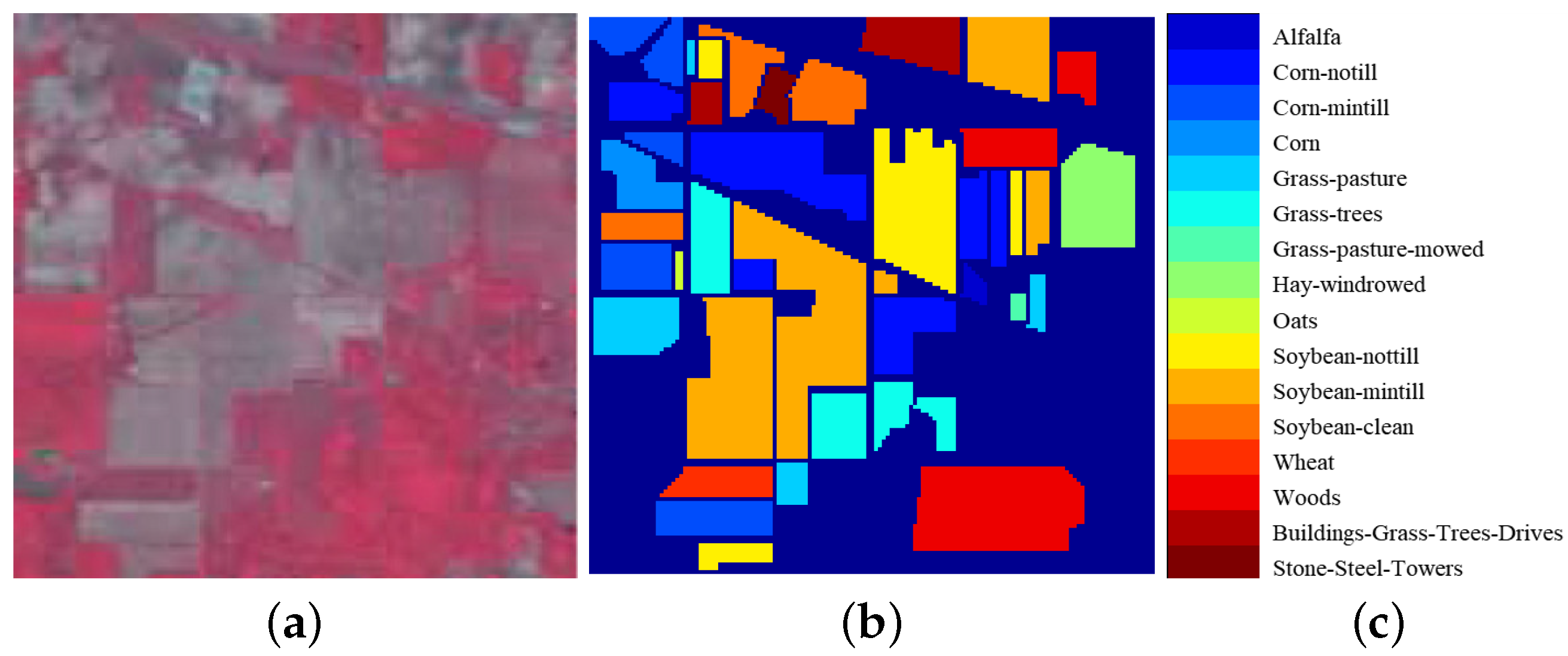
The Indian Pines dataset employed in this study encompasses 16 distinct land feature classes and a total of 220 spectral bands. Typically, the number of bands is reduced to 200 by removing bands covering the region of water absorption; see, e.g., [104–108], [150–163], 220. Figure 2 illustrates the pseudo-color map of the data, along with the class diagram representing the actual features and the corresponding category labels.

Table 1. Indian Pines dataset category information.

Index	Class Name	Sample Size
1	Alfalfa	46
2	Corn-notill	1428
3	Corn-mintill	830
4	Corn	237
5	Grass-pasture	483
6	Grass-trees	730
7	Grass-pasture-mowed	28
8	Hay-windrowed	478
9	Oats	20
10	Soybean-nottill	972
11	Soybean-mintill	2455
12	Soybean-clean	593
13	Wheat	205
14	Woods	1265
15	Buildings-Grass-Trees-Drives	386
16	Stone-Steel-Towers	93

provides detailed category information of the Indian Pines dataset.

4.1.2. Salinas Dataset

The Salinas dataset utilized in this research primarily encompasses land types such as vegetables and fallow land, and a total of 16 categories. For this study, 204 bands were employed for the experimental analysis, excluding the absorption bands. Figure 3 visually presents the pseudo-color map of the data, the class diagram illustrating the actual features, and the corresponding category labels. Detailed category information of the Salinas dataset is provided in

Table 2. Salinas dataset category information.

Index	Class Name	Sample Size
1	Brocoli_green_weeds_1	2009
2	Brocoli_green_weeds_2	3726
3	Fallow	1976
4	Fallow_rough_plow	1394
5	Fallow_smooth	2678
6	Stubble	3959
7	Celery	3579
8	Grapes_untrained	11,271
9	Soil_vinyard_develop	6203
10	Corn_senesced_green_weeds	3278
11	Lettuce_romaine_4wk	1068
12	Lettuce_romaine_5wk	1927
13	Lettuce_romaine_6wk	916
14	Lettuce_romaine_7wk	1070
15	Vinyard_ untrained	7268
16	Vinyard_vertical_trellis	1807

.

4.1.3. PaviaU Dataset

The PaviaU dataset primarily consists of nine categories representing different land features, including asphalt and grassland. Figure 4 provides a pseudo-color map of the data, along with the class diagram depicting the actual features and their corresponding category labels. Detailed category information of the PaviaU dataset is presented in

Table 3. PaviaU dataset category information.

Index	Class Name	Sample Size
1	Asphalt	6631
2	Meadows	18,649
3	Gravel	2099
4	Trees	3064
5	Metal sheets	1345
6	Bare soil	5029
7	Bitumen	1330
8	Bricks	3682
9	Shadows	947

.

4.2. Experimental Results and Analysis

To validate the classification performance of the GSSCRC algorithm, several comparison algorithms, namely, Support Vector Machine (SVM), Sparse Representation Classification (SRC), Kernel Sparse Representation Classification (KSRC), and Joint Cooperative Representation Classification (JCR), are reported in this section. The evaluation criteria used to quantitatively assess the experimental results include average classification accuracy (AA), overall classification accuracy (OA), and kappa coefficient (Kappa).

In the experiments, the selection of the number of neighbors, denoted by k, was set to 7. Specific parameter settings were used for each dataset, where $\lambda =5\times {10}^2$, $\mu =5\times {10}^{-3}, \beta =1\times {10}^2$ for the Indian Pines dataset; $\lambda =1\times {10}^{-2}, \mu =1\times {10}^2,$$\beta =1\times {10}^1$ for the Salinas dataset; and $\lambda =5\times {10}^1, \mu =5\times {10}^1, \beta =1\times {10}^1$ for the PaviaU dataset. For the Indian Pines dataset, 10% of the data were used for training, with the remaining data serving as the test samples. Similarly, for the Salinas dataset, 5% of the data were allocated for training, and for the PaviaU dataset, 10% of the data were used as the training samples. The chosen partitioning strategy was selected to directly reflect the scarcity of labeled hyperspectral data in a real scenario. For each dataset, we dedicated a significant portion to the testing set while allocating a comparatively smaller proportion for training. This deliberate division allows us to effectively assess and validate the performance of the proposed method, even when operating with a restricted number of training samples.

Once the necessary parameters were set, the GSSCRC algorithm could be compared and analyzed against the other algorithms to assess its overall performance. The experimental results are presented in the form of graphs.

Table 4. Detailed classification results of GSSCRC algorithm and other algorithms for various features in the Indian Pines dataset (%).

Category	Sample Size		Classification Methods
	Training Samples	Test Samples	SVM	SRC	KSRC	JCR	GSSCRC
1	5	41	87.96	100	100	100	100
2	143	1285	60.38	81.58	86.97	88.44	90.97
3	83	747	45.36	80.60	84.58	86.50	88.07
4	24	213	42.61	56.12	72.80	78.48	84.39
5	48	435	80.12	90.68	92.75	95.03	95.65
6	73	657	93.65	98.63	97.53	98.76	98.77
7	3	25	92.80	100	100	100	100
8	48	430	88.62	97.48	97.90	99.79	99.79
9	2	18	93.25	100	100	100	100
10	97	875	57.68	81.17	85.70	89.40	90.53
11	246	2209	74.06	82.20	86.27	86.29	86.76
12	59	534	60.85	85.16	88.70	87.18	94.94
13	21	184	93.67	99.02	99.02	99.51	99.51
14	127	1138	90.76	97.87	96.92	97.54	97.63
15	39	347	50.27	62.17	73.83	79.53	79.53
16	9	84	94.38	100	100	100	100
OA (%)			75.40	84.82	88.33	89.92	91.33
AA (%)			77.71	87.34	90.66	92.32	93.81
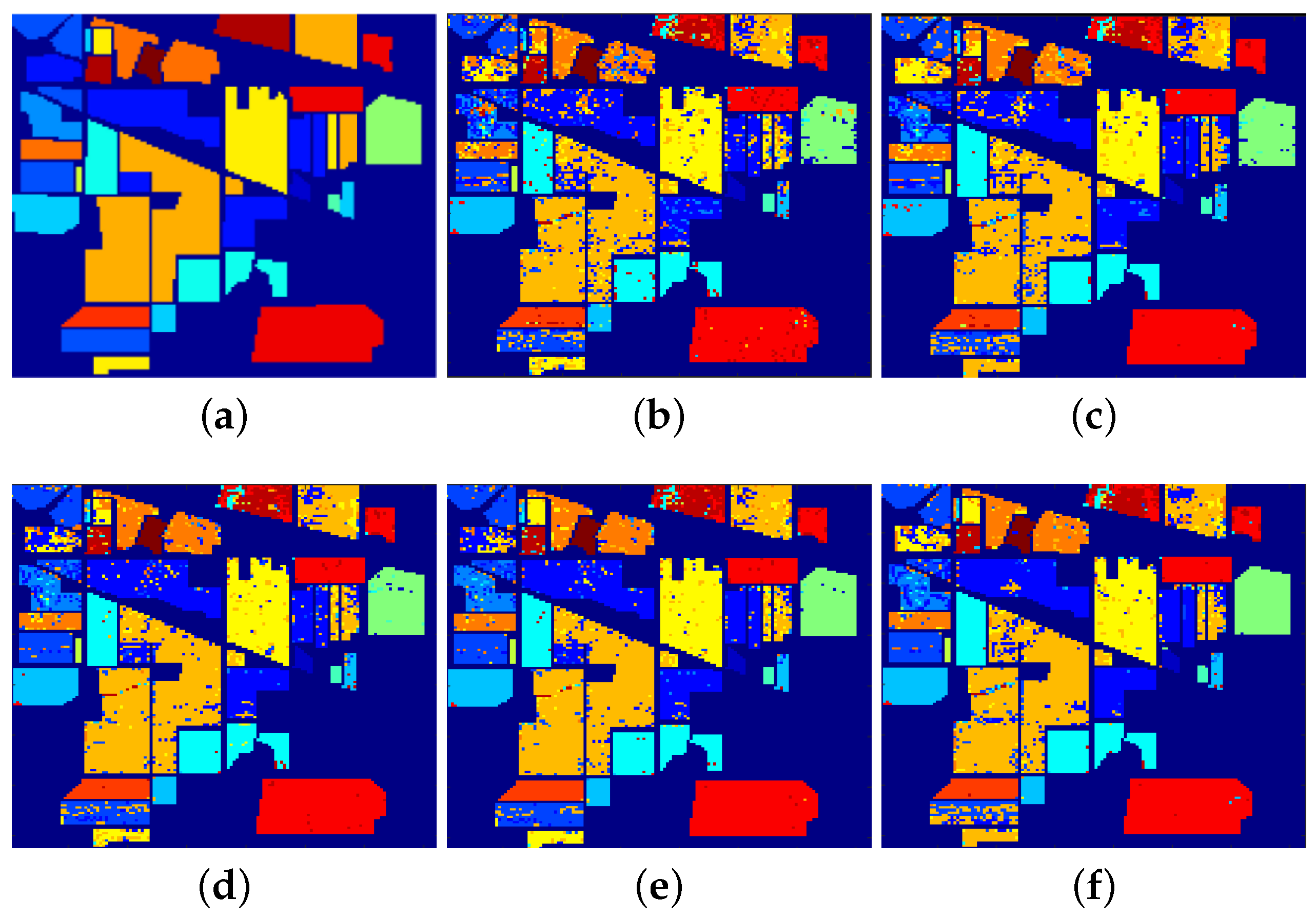
Kappa (%)			73.86	82.68	86.70	88.53	90.13

and Figure 5 provide a detailed overview of the classification results and visualization of the effects achieved by the GSSCRC algorithm and the other algorithms for each feature within the Indian Pines dataset, respectively.

Based on the data presented in Table 4, it is evident that the GSSCRC algorithm proposed in this study exhibits improved classification accuracy for most ground objects compared with other classification methods. In comparison to the SVM, SRC, and KSRC algorithms, which solely utilize spectral information, as well as the JCR algorithm, which incorporates both spatial and spectral information, the GSSCRC algorithm achieved higher OA, AA, and kappa coefficient. These results indicate that by employing geodesic-based spectral neighbor information selection, the GSSCRC algorithm effectively extracts spectral discrimination information. Additionally, the GSSCRC algorithm leverages the combination of spectral and spatial information, enabling it to extract a greater amount of information. Therefore, the GSSCRC algorithm proposed in this study demonstrates promising potential for improving the accurate classification of ground objects.

Figure 5 illustrates the classification results obtained using the GSSCRC algorithm and the comparison algorithms on the Indian Pines dataset. The graph highlights that the algorithm proposed in this study exhibits classification performance that closely resembles the actual terrain map of the Indian Pines dataset. It is observed that the misclassification of terrain pixels is relatively minimal, resulting in a smoother overall effect. Particularly, the algorithm demonstrates superior performance in the classification of the Hay Windrowed and Corn-notill features compared with the other algorithms.

Moving forward, the experiment was conducted on the Salinas dataset. The detailed classification results and the classification effects of the GSSCRC algorithm and other algorithms for different features on the Salinas dataset are presented in

Table 5. Detailed classification results of various features in the Salinas dataset using GSSCRC algorithm and other algorithms (%).

Category	Sample Size		Classification Methods
	Training Samples	Test Samples	SVM	SRC	KSRC	JCR	GSSCRC
1	101	1908	99.65	99.25	99.60	99.70	100
2	187	3539	97.69	98.87	99.97	100	100
3	99	1877	98.93	98.38	99.79	99.70	99.80
4	70	1324	99.56	99.64	100	99.71	99.92
5	144	2648	96.71	98.84	98.58	98.14	99.10
6	198	3761	99.04	99.62	99.62	99.72	99.72
7	179	3400	99.46	99.61	99.80	99.86	99.86
8	564	10,707	80.25	96.51	81.68	89.62	89.76
9	311	6173	99.45	97.34	99.84	99.98	100
10	164	3248	90.91	96.92	97.83	98.28	98.32
11	54	1012	94.75	99.53	99.91	98.60	98.65
12	97	1830	98.91	100	100	100	100
13	46	870	99.56	97.92	99.45	99.12	99.13
14	54	1016	80.56	98.59	99.34	95.70	95.70
15	364	7238	97.48	97.33	96.79	78.23	77.43
16	91	1716	96.84	99.33	99.61	99.43	99.45
OA (%)			89.34	91.19	92.21	94.45	95.62
AA (%)			93.21	95.81	96.76	97.28	97.30
Kappa(%)			88.15	90.19	91.33	93.76	93.84

and Figure 6, respectively.

Based on the data presented in Table 5, it is evident that the GSSCRC algorithm proposed in this paper significantly improved the classification accuracy compared with other classification methods. Furthermore, the GSSCRC algorithm exhibited slightly higher values for OA, AA, and Kappa coefficient when compared with other algorithms. Notably, the algorithm demonstrated correct classification of ground objects of class 1 and class 9, indicating the beneficial effect of geodesic distance on selecting spectral nearest-neighbor information and affirming the effectiveness of the algorithm.

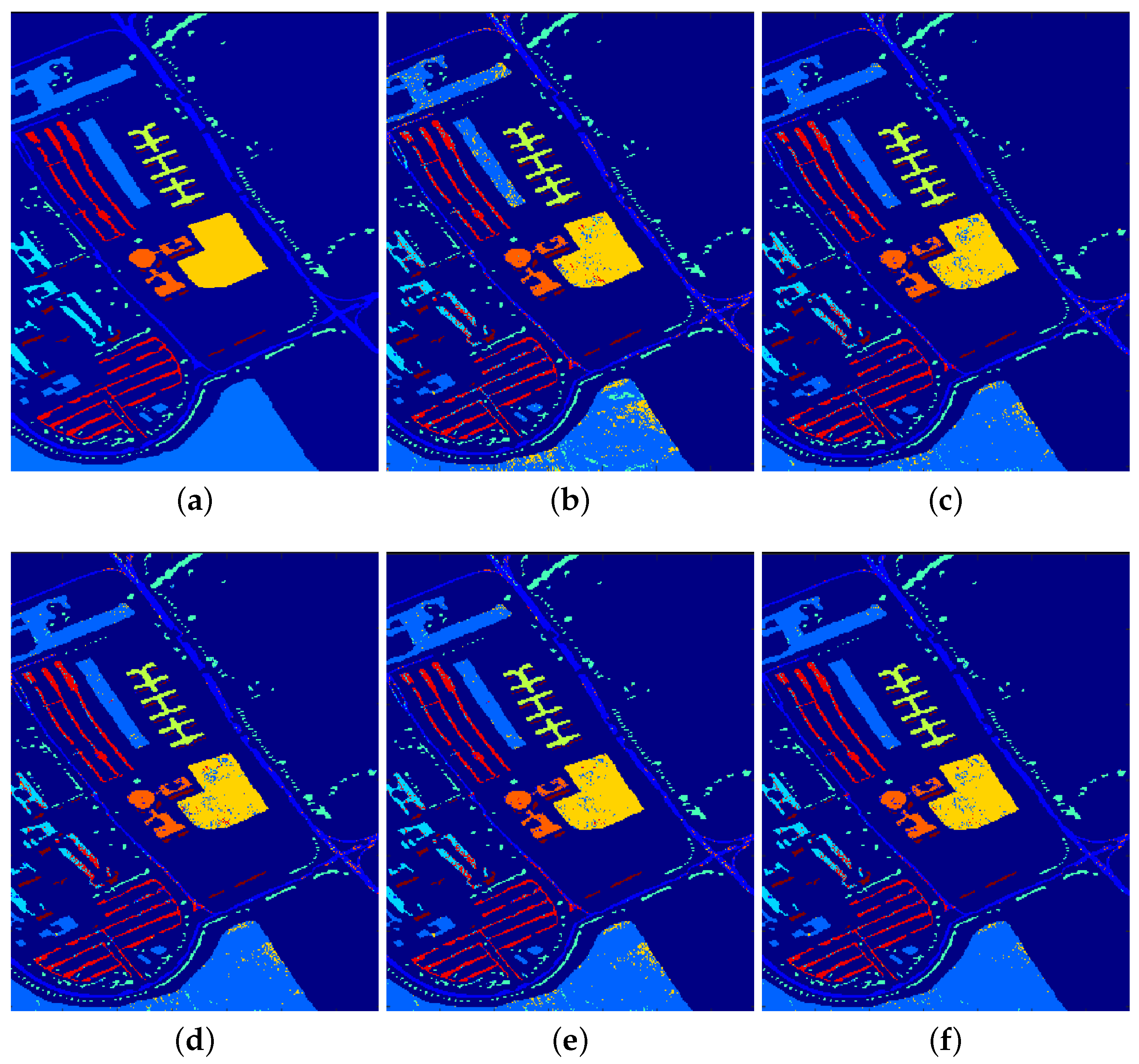
Figure 6 provides a visual representation of the classification performance of the GSSCRC algorithm and the comparison algorithms on the Salinas dataset. Upon analyzing the classification performance of each algorithm, it can be concluded that the algorithm proposed in this study achieved classification results that closely resemble the real terrain map of the Salinas dataset. The algorithm exhibited fewer misclassifications in the dataset, resulting in a smoother overall effect. Particularly, in the classification of the weeds1 and Soil land features, the performance of the GSSCRC algorithm surpassed that of other algorithms. This observation highlights the capability of the GSSCRC algorithm of extracting spectral information more comprehensively with the usage of geodesic distance for selecting spectral nearest-neighbor information. By incorporating spatial information from hyperspectral images, the algorithm effectively captures the deep characteristics of hyperspectral image data.

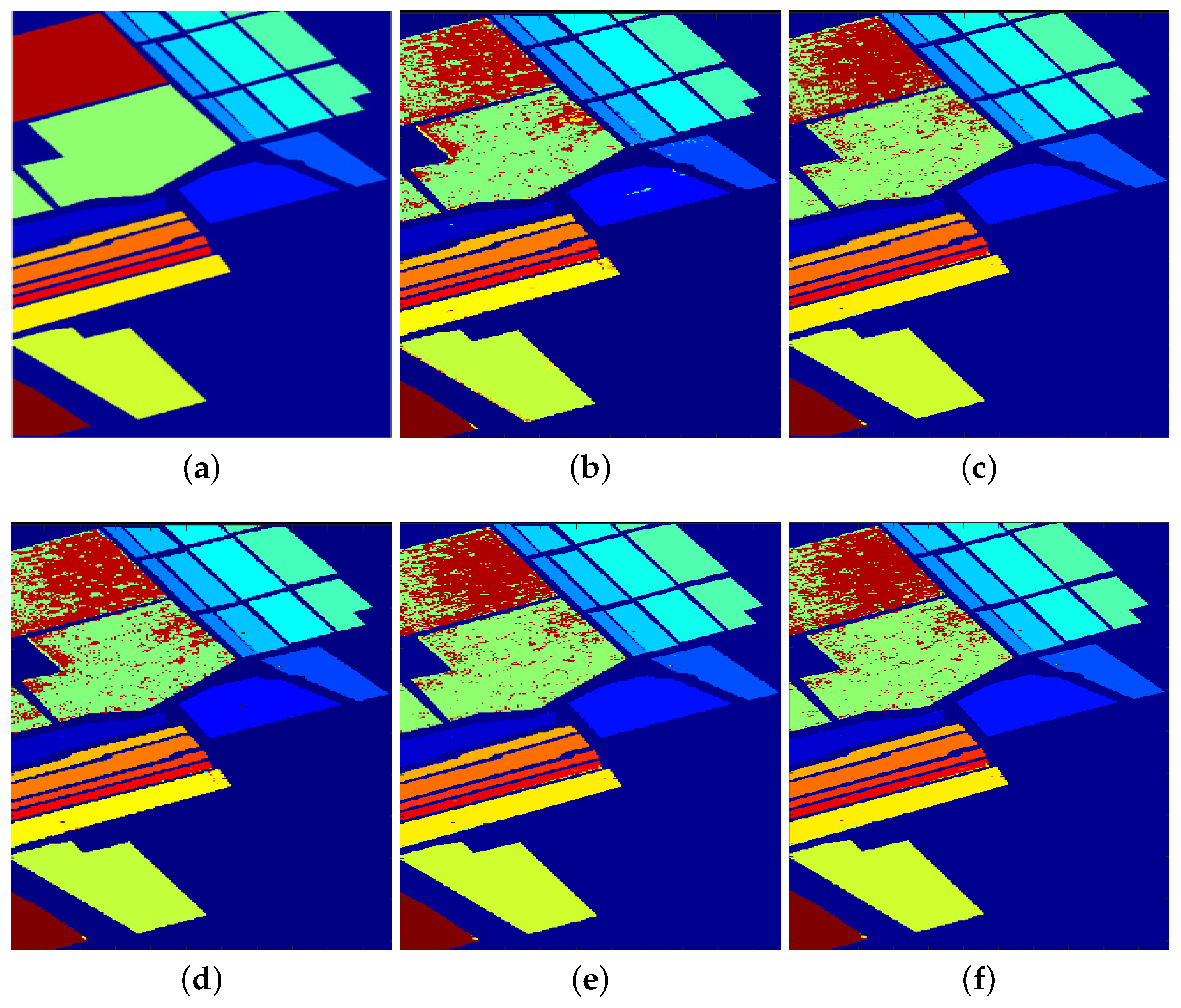
To further validate the effectiveness of the GSSCRC algorithm, experiments were conducted on the PaviaU dataset. The detailed classification results and classification effects of the GSSCRC algorithm, along with those of other algorithms, are presented in

Table 6. Detailed classification results of GSSCRC algorithm and other algorithms for various features in the PaviaU dataset (%).

Category	Sample Size		Classification Methods
	Training Samples	Test Samples	SVM	SRC	KSRC	JCR	GSSCRC
1	663	5968	86.79	92.76	91.38	92.09	96.20
2	1864	16,785	88.78	96.65	96.75	95.93	98.44
3	210	1889	83.33	82.56	75.27	81.89	83.66
4	306	2758	97.81	96.41	96.41	96.96	96.21
5	135	1210	99.63	99.70	99.18	99.63	99.63
6	503	4526	93.39	91.91	90.97	94.65	93.82
7	133	1197	93.98	90.98	92.93	92.26	90.60
8	368	3314	85.85	88.29	91.01	92.50	91.91
9	95	852	100	99.89	100	99.89	99.89
OA (%)			89.81	93.86	93.35	94.18	95.77
AA (%)			91.99	92.98	92.14	93.73	94.13
Kappa (%)			86.77	91.88	91.21	92.33	94.38

and Figure 7, respectively.

From the data in Table 6, it is evident that the GSSCRC algorithm proposed in this paper significantly improved the classification accuracy compared with other classification methods. The OA, AA, and Kappa coefficient of the GSSCRC algorithm are slightly higher than those of other algorithms, indicating the effectiveness of using geodesic distance in the selection of spectral nearest-neighbor information.

Figure 7 presents the classification effect maps of the GSSCRC algorithm and the comparison algorithms on the PaviaU dataset. By observing the classification effect map of each algorithm, it can be concluded that in the Asphalt, Meadow, and Gravel regions, there are fewer misclassified pixels of ground features compared with the comparison algorithms, resulting in a smoother overall effect map. This demonstrates that the GSSCRC algorithm proposed in this paper can effectively reveal the intrinsic features hidden behind a hyperspectral image by combining the geodesic-based spectral information and spatial information.

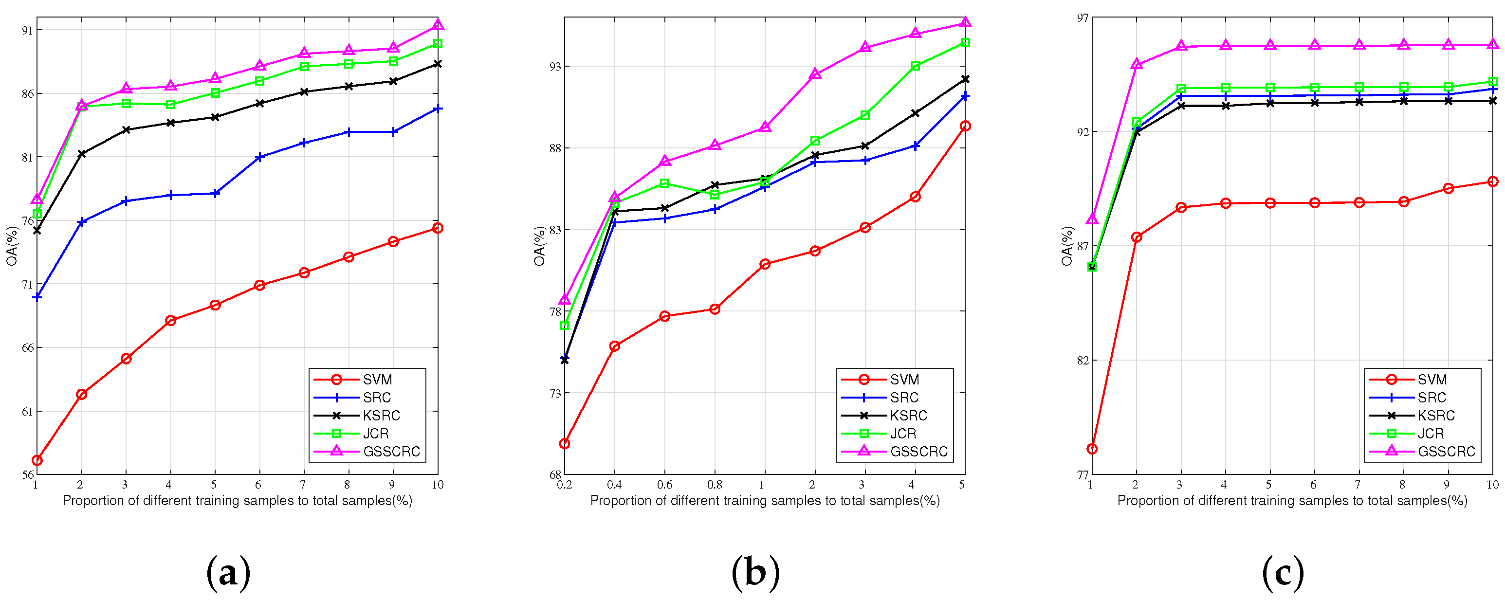
In order to examine the impact of the GSSCRC algorithm, as well as that of the SVM, SRC, KSRC, and JCR algorithms, on the overall classification results with varying numbers of training samples, this study conducts experiments on three datasets to assess the influence of different training sample sizes. For the Indian Pines dataset, the selected training sample proportions range from 1% to 10%, with the remaining samples being used as the test sample set. Similarly, for the Salinas dataset, the proportions range from 0.2% to 5%, and for the PaviaU dataset, the proportions range from 1% to 10%. The effect of different training sample sizes on the classification performance is depicted in Figure 8.

Figure 8 illustrates the impact of different algorithms on the overall classification accuracy with varying training sample sizes across the three datasets. From Figure 8a–c, it is evident that as the proportion of training datasets increases, the OA values of each algorithm also increase correspondingly.

To compare the running time of the GSSCRC algorithm with that of the SVM, SRC, KSRC, and JCR algorithms,

Table 7. Running time of GSSCRC and comparison algorithm on different datasets (s).

Method	Indian Pines Dataset	Salinas Dataset	PaviaU Dataset
SVM	293.97	2168.53	1301.62
SRC	334.91	2865.72	1425.13
KSRC	338.34	4114.06	1476.75
JCR	348.08	4800.50	1685.32
GSSCRC	365.36	5176.28	2244.06

presents the running time results of GSSCRC and the comparison algorithms on different datasets. It can be observed that SVM had the shortest running time, followed by the SRC, KSRC, and JCR algorithms. However, the GSSCRC algorithm in this paper had the longest running time due to the additional computational resources required for spectral information nearest-neighbor selection. Furthermore, the computation of the regularization term based on the competitive representation of spatial and spectral information also contributes to the increased computational cost. It is expected that the efficiency of the algorithm can be improved by combining some optimization methods [48,49]. Image processing combined with machine learning [50,51] may also bring some improvements. Despite the higher computational resource consumption, the GSSCRC algorithm demonstrates satisfactory classification performance, surpassing other similar algorithms in various aspects.

5. Conclusions

This paper presents the GSSCRC algorithm for hyperspectral image classification. The algorithm incorporates the cooperative representation classification model and introduces the geodesic distance calculation method to select spectral nearest-neighbor information, thereby effectively utilizing the neighbor information in hyperspectral images. By integrating spatial information and spectral information based on geodesic distance, the algorithm effectively harnesses the spatial–spectral characteristics inherent in hyperspectral images. Specifically, the regularization term of the traditional collaborative representation model is enhanced by incorporating spatial proximity information and spectral information based on geodesic distance, resulting in the derivation of a geodesic-constrained spatial–spectral collaborative representation coefficient matrix. This approach facilitates the exploration and utilization of the spatial–spectral neighborhood structure of hyperspectral data, enabling the effective extraction of deep features. Experimental results demonstrate that the proposed algorithm outperforms the SVM, SRC, KSRC, and JCR algorithms in ground-object classification performance. The hyperspectral image data classification method proposed in this study is specifically designed to handle the complexities introduced by high-dimensional data in hyperspectral remote sensing in the era of big data, where the fusion of spectral and spatial information plays a crucial role in achieving accurate and efficient classification. While the classification methods we introduced demonstrate promising outcomes in hyperspectral image classification, it is important to note that the proposed algorithm’s applicability beyond this context has not been explored yet. In future research, we could try to validate the performance of the proposed algorithm on other hyperspectral datasets and improve it.

References

1. Toth, C.; Jozkow, G. Remote sensing platforms and sensors: A survey. ISPRS J. Photogramm. Remote Sens. 2016, 115, 22–36. [Google Scholar] [CrossRef]
2. Ning, Z.; Dong, P.; Wang, X.; Hu, X.; Guo, L.; Hu, B.; Guo, Y.; Qiu, T.; Kwok, R.Y.K. Mobile Edge Computing Enabled 5G Health Monitoring for Internet of Medical Things: A Decentralized Game Theoretic Approach. IEEE J. Sel. Areas Commun. 2021, 39, 463–478. [Google Scholar] [CrossRef]
3. Ning, Z.; Chen, H.; Ngai, E.C.H.; Wang, X.; Guo, L.; Liu, J. Lightweight Imitation Learning for Real-Time Cooperative Service Migration. IEEE Trans. Mob. Comput. 2023, 1–18. [Google Scholar] [CrossRef]
4. Ning, Z.; Dong, P.; Wang, X.; Rodrigues, J.J.P.C.; Xia, F. Deep Reinforcement Learning for Vehicular Edge Computing: An Intelligent Offloading System. ACM Trans. Intell. Syst. Technol. 2019, 10, 60. [Google Scholar] [CrossRef]
5. Pu, H.; Chen, Z.; Wang, B.; Jiang, G.M. A Novel Spatial–Spectral Similarity Measure for Dimensionality Reduction and Classification of Hyperspectral Imagery. IEEE Trans. Geosci. Remote Sens. 2014, 52, 7008–7022. [Google Scholar] [CrossRef]
6. Chen, Y.; Zhu, K.; Zhu, L.; He, X.; Ghamisi, P.; Benediktsson, J.A. Automatic Design of Convolutional Neural Network for Hyperspectral Image Classification. IEEE Trans. Geosci. Remote Sens. 2019, 57, 7048–7066. [Google Scholar] [CrossRef]
7. Ning, Z.; Zhang, K.; Wang, X.; Obaidat, M.S.; Guo, L.; Hu, X.; Hu, B.; Guo, Y.; Sadoun, B.; Kwok, R.Y.K. Joint Computing and Caching in 5G-Envisioned Internet of Vehicles: A Deep Reinforcement Learning-Based Traffic Control System. IEEE Trans. Intell. Transp. Syst. 2021, 22, 5201–5212. [Google Scholar] [CrossRef]
8. Ning, Z.; Zhang, K.; Wang, X.; Guo, L.; Hu, X.; Huang, J.; Hu, B.; Kwok, R.Y.K. Intelligent Edge Computing in Internet of Vehicles: A Joint Computation Offloading and Caching Solution. IEEE Trans. Intell. Transp. Syst. 2021, 22, 2212–2225. [Google Scholar] [CrossRef]
9. Wan, L.; Li, X.; Xu, J.; Sun, L.; Wang, X.; Liu, K. Application of Graph Learning with Multivariate Relational Representation Matrix in Vehicular Social Networks. IEEE Trans. Intell. Transp. Syst. 2023, 24, 2789–2799. [Google Scholar] [CrossRef]
10. Paoletti, M.E.; Haut, J.M.; Plaza, J.; Plaza, A. Deep learning classifiers for hyperspectral imaging: A review. ISPRS J. Photogramm. Remote Sens. 2019, 158, 279–317. [Google Scholar] [CrossRef]
11. Honkavaara, E.; Rosnell, T.; Oliveira, R.; Tommaselli, A. Band registration of tuneable frame format hyperspectral UAV imagers in complex scenes. ISPRS J. Photogramm. Remote Sens. 2017, 134, 96–109. [Google Scholar] [CrossRef]
12. Ning, Z.; Hu, H.; Wang, X.; Guo, L.; Guo, S.; Wang, G.; Gao, X. Mobile Edge Computing and Machine Learning in the Internet of Unmanned Aerial Vehicles: A Survey. ACM Comput. Surv. 2023, 56, 13. [Google Scholar] [CrossRef]
13. Wang, X.; Ning, Z.; Guo, S.; Wen, M.; Guo, L.; Poor, H.V. Dynamic UAV Deployment for Differentiated Services: A Multi-Agent Imitation Learning Based Approach. IEEE Trans. Mob. Comput. 2023, 22, 2131–2146. [Google Scholar] [CrossRef]
14. Ning, Z.; Yang, Y.; Wang, X.; Guo, L.; Gao, X.; Guo, S.; Wang, G. Dynamic Computation Offloading and Server Deployment for UAV-Enabled Multi-Access Edge Computing. IEEE Trans. Mob. Comput. 2023, 22, 2628–2644. [Google Scholar] [CrossRef]
15. Sun, L.; Wan, L.; Wang, J.; Lin, L.; Gen, M. Joint Resource Scheduling for UAV-Enabled Mobile Edge Computing System in Internet of Vehicles. IEEE Trans. Intell. Transp. Syst. 2022, 1–9. [Google Scholar] [CrossRef]
16. Wang, X.; Li, J.; Ning, Z.; Song, Q.; Guo, L.; Guo, S.; Obaidat, M.S. Wireless Powered Mobile Edge Computing Networks: A Survey. ACM Comput. Surv. 2023, 55, 263. [Google Scholar] [CrossRef]
17. Sun, H.; Zheng, X.; Lu, X.; Wu, S. Spectral–Spatial Attention Network for Hyperspectral Image Classification. IEEE Trans. Geosci. Remote Sens. 2020, 58, 3232–3245. [Google Scholar] [CrossRef]
18. Zhang, L.; Yang, M.; Feng, X. Sparse representation or collaborative representation: Which helps face recognition? In Proceedings of the 2011 International Conference on Computer Vision, Barcelona, Spain, 6–13 November 2011; pp. 471–478. [Google Scholar] [CrossRef]
19. Su, H.; Yu, Y.; Wu, Z.; Du, Q. Random Subspace-Based k-Nearest Class Collaborative Representation for Hyperspectral Image Classification. IEEE Trans. Geosci. Remote Sens. 2021, 59, 6840–6853. [Google Scholar] [CrossRef]
20. Su, H.; Gao, Y.; Du, Q. Superpixel-Based Relaxed Collaborative Representation with Band Weighting for Hyperspectral Image Classification. IEEE Trans. Geosci. Remote Sens. 2022, 60, 1–16. [Google Scholar] [CrossRef]
21. Abuassba, A.O.M.; Dezheng, Z.; Ali, H.; Zhang, F.; Ali, K. Classification with ensembles and case study on functional magnetic resonance imaging. Digit. Commun. Netw. 2022, 8, 80–86. [Google Scholar] [CrossRef]
22. Mousavi, S.N.; Chen, F.; Abbasi, M.; Khosravi, M.R.; Rafiee, M. Efficient pipelined flow classification for intelligent data processing in IoT. Digit. Commun. Netw. 2022, 8, 561–575. [Google Scholar] [CrossRef]
23. Ning, Z.; Xia, F.; Ullah, N.; Kong, X.; Hu, X. Vehicular Social Networks: Enabling Smart Mobility. IEEE Commun. Mag. 2017, 55, 16–55. [Google Scholar] [CrossRef]
24. Wang, X.; Ning, Z.; Guo, S.; Wang, L. Imitation Learning Enabled Task Scheduling for Online Vehicular Edge Computing. IEEE Trans. Mob. Comput. 2022, 21, 598–611. [Google Scholar] [CrossRef]
25. Peng, J.; Li, L.; Tang, Y.Y. Maximum Likelihood Estimation-Based Joint Sparse Representation for the Classification of Hyperspectral Remote Sensing Images. IEEE Trans. Neural Netw. Learn. Syst. 2019, 30, 1790–1802. [Google Scholar] [CrossRef] [PubMed]
26. Ma, L.; Crawford, M.M.; Tian, J. Local Manifold Learning-Based k -Nearest-Neighbor for Hyperspectral Image Classification. IEEE Trans. Geosci. Remote Sens. 2010, 48, 4099–4109. [Google Scholar] [CrossRef]
27. Xia, J.; Bombrun, L.; Adalı, T.; Berthoumieu, Y.; Germain, C. Spectral–Spatial Classification of Hyperspectral Images Using ICA and Edge-Preserving Filter via an Ensemble Strategy. IEEE Trans. Geosci. Remote Sens. 2016, 54, 4971–4982. [Google Scholar] [CrossRef]
28. Jia, S.; Zhao, Q.; Zhuang, J.; Tang, D.; Long, Y.; Xu, M.; Zhou, J.; Li, Q. Flexible Gabor-Based Superpixel-Level Unsupervised LDA for Hyperspectral Image Classification. IEEE Trans. Geosci. Remote Sens. 2021, 59, 10394–10409. [Google Scholar] [CrossRef]
29. Melgani, F.; Bruzzone, L. Classification of hyperspectral remote sensing images with support vector machines. IEEE Trans. Geosci. Remote Sens. 2004, 42, 1778–1790. [Google Scholar] [CrossRef]
30. Li, W.; Chen, C.; Su, H.; Du, Q. Local Binary Patterns and Extreme Learning Machine for Hyperspectral Imagery Classification. IEEE Trans. Geosci. Remote Sens. 2015, 53, 3681–3693. [Google Scholar] [CrossRef]
31. Guo, A.J.X.; Zhu, F. Spectral-Spatial Feature Extraction and Classification by ANN Supervised With Center Loss in Hyperspectral Imagery. IEEE Trans. Geosci. Remote Sens. 2019, 57, 1755–1767. [Google Scholar] [CrossRef]
32. Gao, Q.; Lim, S.; Jia, X. Hyperspectral Image Classification Using Joint Sparse Model and Discontinuity Preserving Relaxation. IEEE Geosci. Remote Sens. Lett. 2018, 15, 78–82. [Google Scholar] [CrossRef]
33. Li, J.; Zhang, H.; Zhang, L. Column-generation kernel nonlocal joint collaborative representation for hyperspectral image classification. ISPRS J. Photogramm. Remote Sens. 2014, 94, 25–36. [Google Scholar] [CrossRef]
34. Wang, X.; Ning, Z.; Guo, L.; Guo, S.; Gao, X.; Wang, G. Mean-Field Learning for Edge Computing in Mobile Blockchain Networks. IEEE Trans. Mob. Comput. 2022, 1–17. [Google Scholar] [CrossRef]
35. Ning, Z.; Sun, S.; Wang, X.; Guo, L.; Guo, S.; Hu, X.; Hu, B.; Kwok, R.Y.K. Blockchain-Enabled Intelligent Transportation Systems: A Distributed Crowdsensing Framework. IEEE Trans. Mob. Comput. 2022, 21, 4201–4217. [Google Scholar] [CrossRef]
36. Wang, X.; Zhu, H.; Ning, Z.; Guo, L.; Yan, Z. Blockchain Intelligence for Internet of Vehicles: Challenges and Solutions. IEEE Commun. Surv. Tutor. 2023, 1. [Google Scholar] [CrossRef]
37. Donoho, D.L.; Tanner, J. Sparse nonnegative solution of underdetermined linear equations by linear programming. Proc. Natl. Acad. Sci. USA 2005, 102, 9446–9451. [Google Scholar] [CrossRef]
38. Wright, J.; Yang, A.Y.; Ganesh, A.; Sastry, S.S.; Ma, Y. Robust Face Recognition via Sparse Representation. IEEE Trans. Pattern Anal. Mach. Intell. 2009, 31, 210–227. [Google Scholar] [CrossRef] [PubMed]
39. Tang, Y.Y.; Yuan, H.; Li, L. Manifold-Based Sparse Representation for Hyperspectral Image Classification. IEEE Trans. Geosci. Remote Sens. 2014, 52, 7606–7618. [Google Scholar] [CrossRef]
40. Chen, Y.; Nasrabadi, N.M.; Tran, T.D. Hyperspectral Image Classification Using Dictionary-Based Sparse Representation. IEEE Trans. Geosci. Remote Sens. 2011, 49, 3973–3985. [Google Scholar] [CrossRef]
41. Chen, X.; Li, S.; Peng, J. Hyperspectral Imagery Classification with Multiple Regularized Collaborative Representations. IEEE Geosci. Remote Sens. Lett. 2017, 14, 1121–1125. [Google Scholar] [CrossRef]
42. Li, W.; Du, Q.; Xiong, M. Kernel Collaborative Representation With Tikhonov Regularization for Hyperspectral Image Classification. IEEE Geosci. Remote Sens. Lett. 2015, 12, 48–52. [Google Scholar] [CrossRef]
43. Willoughby, R.A. Solutions of Ill-Posed Problems (A. N. Tikhonov and V. Y. Arsenin). SIAM Rev. 1979, 21, 266–267. [Google Scholar] [CrossRef]
44. Li, J.; Zhang, H.; Zhang, L.; Huang, X.; Zhang, L. Joint Collaborative Representation With Multitask Learning for Hyperspectral Image Classification. IEEE Trans. Geosci. Remote Sens. 2014, 52, 5923–5936. [Google Scholar] [CrossRef]
45. Xiong, M.; Ran, Q.; Li, W.; Zou, J.; Du, Q. Hyperspectral Image Classification Using Weighted Joint Collaborative Representation. IEEE Geosci. Remote Sens. Lett. 2015, 12, 1209–1213. [Google Scholar] [CrossRef]
46. Yang, J.; Qian, J. Hyperspectral Image Classification via Multiscale Joint Collaborative Representation with Locally Adaptive Dictionary. IEEE Geosci. Remote Sens. Lett. 2018, 15, 112–116. [Google Scholar] [CrossRef]
47. Peng, Z.; Dong, Y.; Luo, M.; Wu, X.M.; Zheng, Q. A new self-supervised task on graphs: Geodesic distance prediction. Inf. Sci. 2022, 607, 1195–1210. [Google Scholar] [CrossRef]
48. Wang, X.; Ning, Z.; Wang, L. Offloading in Internet of Vehicles: A Fog-Enabled Real-Time Traffic Management System. IEEE Trans. Ind. Inform. 2018, 14, 4568–4578. [Google Scholar] [CrossRef]
49. Ning, Z.; Dong, P.; Kong, X.; Xia, F. A Cooperative Partial Computation Offloading Scheme for Mobile Edge Computing Enabled Internet of Things. IEEE Internet Things J. 2019, 6, 4804–4814. [Google Scholar] [CrossRef]
50. Zhang, L.; Wang, Z.; Wang, L.; Zhang, Z.; Chen, X.; Meng, L. Machine learning-based real-time visible fatigue crack growth detection. Digit. Commun. Netw. 2021, 7, 551–558. [Google Scholar] [CrossRef]
51. Manning, K.; Zhai, X.; Yu, W. Image analysis and machine learning-based malaria assessment system. Digit. Commun. Netw. 2022, 8, 132–142. [Google Scholar] [CrossRef]
Figure 1. GSSCRC algorithm flowchart.
Electronics 12 03777 g001
Figure 2. Indian Pines dataset: (a) pseudo-color images, (b) real terrain maps, (c) category labels.
Electronics 12 03777 g002
Figure 3. Salinas dataset: (a) pseudo-color image, (b) class diagram of real features, (c) category labels.
Electronics 12 03777 g003
Figure 4. PaviaU dataset: (a) pseudo-color image, (b) class diagram of real features, (c) category labels.
Electronics 12 03777 g004
Figure 5. Classification performance of GSSCRC algorithm and other algorithms on the Indian Pines dataset: (a) ground truth, (b) SVM, (c) SRC, (d) KSRC, (e) JCR, (f) GSSCRC.
Electronics 12 03777 g005
Figure 6. Classification performance of GSSCRC algorithm and other algorithms on the Salinas dataset: (a) ground truth, (b) SVM, (c) SRC, (d) KSRC, (e) JCR, (f) GSSCRC.
Electronics 12 03777 g006
Figure 7. Classification effects of GSSCRC algorithm and other algorithms on PaviaU dataset: (a) ground truth, (b) SVM, (c) SRC, (d) KSRC, (e) JCR, (f) GSSCRC.
Electronics 12 03777 g007
Figure 8. Impact of different algorithms on overall classification accuracy with different training sample sizes: (a) Indian Pines dataset, (b) Salinas dataset, (c) PaviaU dataset.
Electronics 12 03777 g008