An Analytical Model of a System with Compression and Queuing for Selected Traffic Flows

Abstract

This article proposes a new analytical model of a queuing system to which a mixture of multi-service traffic is offered. The system under consideration has the advantage of servicing calls, in a shared server, of which only part will be placed in a queue when the server has no free resources (while the remaining part of the calls will be lost). In addition, this model also introduces the possibility for a compression mechanism to be applied for a selected number of data flows. The possibility of simultaneous analysis of the calls that can be placed in the queue as well as of those in which queuing is not implemented, while a certain number of them can be compressed, provides unquestionable advantage to the proposed model. The proposed model can be successfully applied to analyse and model 5G systems.

1. Introduction

The dynamic development of IT systems and communications and computer networks has the capacity to offer more and more complex services to users. In its classic form, the execution of a service has been related to the transfer of required data between the end-user’s device and the server. Today, the execution of a service is increasingly more complex and, in effect, requires processing of data in a number of different elements of a communications system. Such an approach must be followed by a redefinition of the resources necessary for the execution of a given service, since besides the required bitrate and calculational power, the actual place of partial or total data processing has to be designated. This, in turn, makes it necessary for network operators to employ more and more sophisticated traffic management mechanisms that would take into consideration the changes in the characteristics of data streams that follow their partial processing [1,2,3].

For years, network operators have been successfully implementing a number of various mechanisms that make it possible to optimise the use of available network resources. One such mechanism is compression [4,5,6,7], which makes it possible to introduce changes in the speed of generating data by its source in order to adjust or accommodate it to the current load of the network. In the case where overload is unavoidable, data can be placed in buffers (queuing mechanism) [8,9]. However, it is also important to take into consideration the fact that not all data streams can be additionally delayed because of a number of time constraints for a given service to which they are related. A good example of the above is the services that are offered in 5G networks. The concept of 5G network services is based on slices, i.e., dedicated “sub-networks” designed for specific solutions that can be characterised by different QoS (Quality of Service) parameters, such as delay (latency), jitter, transmission rate, or the number of serviced devices. Current 5G implementations consider, for example, deployment of scenarios such as the eMBB (Enhanced Mobile Broadband), which in fact is the access network for users, URLLC (Ultra-Reliable Low Latency Communications), dedicated for those solutions in which the most important feature is high reliability and very low latency with moderate transmission rates (as opposed to other scenarios), and MMTC (Massive Machine Type Communications), dedicated to solutions for the Internet of Things (IoT) and the industrial Internet of Things (IIoT) [2].

One of the services currently being worked on by a sizeable number of research and industrial centres is the expected provision of autonomous vehicles (using the URLLC scenario). The report published by Ericsson [10] clearly states that autonomous vehicles will soon become reality. What seems to be the barrier now is a timely appropriate and relevant provision of transmission rates with required latency values. The report claims that each vehicle will generate about 383 Gb per hour, which gives nearly 100 Mbps. The data transmitted by autonomous vehicles can be divided into two groups. The first group is the data related to the provision of proper operation of each of the vehicles (safe roadability, distance from other vehicles, and data sourcing from multiple road sensor infrastructure). The other group is constituted of the data related to the provision of the required (or assumed) comfort of travellers, e.g., current information, access to social media, or access to audio and video content. Data related to the first group constitute sensitive data and as such cannot be delayed, just as their transmission rates cannot be limited in any way. Data that belong to the second group can be delayed and their transmission rates can undergo changes depending on the load of the network. Designing and optimisation of this system require then a development of dedicated analytical models that would allow the required parameters to be assessed in real time. The present article proposes a model of this type of system.

The analytical model proposed in this article has the advantage of providing the possibility of simultaneous analysis of the two types of data serviced by a communications system, e.g., in the radio interface of a 5G network. The first type of data cannot be delayed more than it results from the time needed for its processing (i.e., data cannot be placed in the queue), the second can be additionally delayed and can undergo compression processing (which, of course, induces a change in their transmission rates). The model proposed in the article pertains to the steady state condition, arising from the analysis of the so-called macrostates, i.e., states defined by the total number of occupied resources within the system [8]. In addition, the model introduces efficient constraints for the R resources that can be occupied by compressed traffic. Thanks to this approach, the model can be successfully applied to analyse those slices of a 5G network that are responsible for the service of autonomous vehicles.

Research into multi-service systems with compression and/or queuing is not the only ongoing research in contemporary research centres. It is worth highlighting studies that examine the properties of systems to which BPP traffic is offered [7,9,11,12,13,14]. Analysing systems with BPP traffic allows for the inclusion of the actual number of traffic sources (e.g., network user devices) in analytical models. Single-service queuing systems are also under consideration [15,16,17,18,19,20], which is generally relevant for packet-level system analysis.

The remaining part of this article is structured as follows: Section 2 presents the way in which the resources of the system under consideration and the call demands are represented in the analytical model. Section 3 describes the proposed analytical model. Since the proposed analytical model is an approximate model, Section 4 provides a comparison of the results obtained on the basis of the analytical model with those of a digital simulation. Section 5 sums up the article.

2. Resources and Traffic in Communications Networks

2.1. Resources of the Network

Data transmission in modern-day networks is based on IP packet transmission, while the transmission rates required to execute individual services and the capacity of links are expressed in bps [10,21]. The analysis at the packet level though is complicated and relevant analytical models need to be computationally complex. To simplify the analysis of a system, the so-called discretisation of resources is typically used. As a result, the capacity of a communications system and the requirements for individual services can be expressed in non-dimensional, so-called allocation units—AU (Allocation Unit). The resource discretisation process itself is well known and widely described in the literature, while its basic parameter is the so-called equivalent bandwidth. Determination of the equivalent bandwidth makes it possible to express the data stream, variable in execution time for a given service, by a given constant value that influences the operation of the system in exactly the same way as the considered data stream. The value of the equivalent bandwidth can be determined using appropriate formulae or, for simplifying reasons, can be assumed to be the maximum required transmission rate that is characteristic for a given service. Even though this approach results in significant inaccuracies in developed analytical or simulation models, because of its simplicity and the straightforwardness of the approach, it is becoming increasingly common. This process is extensively and thoroughly discussed in the literature of the subject, e.g., in [22,23]. By having the knowledge of the equivalent bandwidth for all services executed in a system under consideration, the allocation unit AU ($c_{AU}$) can be determined as the greatest common divisor of all equivalent bandwidths determined for each of the services:

$$c_{AU}\le gcd\left\{c_1,\dots ,c_m\right\},$$

(1)

where:

m—number of services,

$c_i$—equivalent bandwidth determined for service $i,1\le i\le m$.

With the knowledge of $c_{AU}$, by simple transformations, it is possible to express the system capacity V in these units as well as the demands for individual services $t_i$:

$$t_i=⌈\frac{c_i}{c_{AU}}⌉,$$

(2)

$$V=⌊\frac{C}{c_{AU}}⌋,$$

(3)

where C is the capacity of the system expressed in bps.

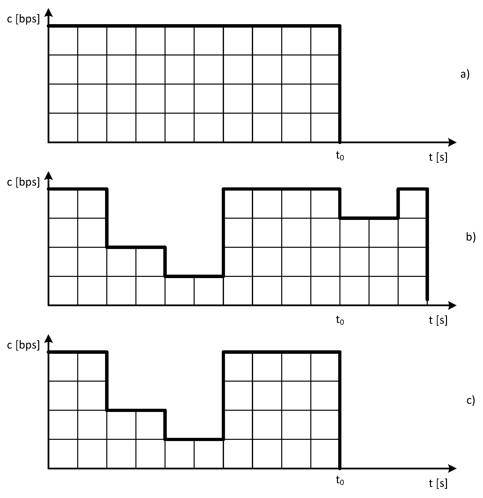
2.2. Traffic in Communications Networks

In modern-day networks, data are transmitted in packets with constant or variable transmission rate. The network analysis at the packet level, even though it leads to accurate and precise solutions, is only temporarily effective, as the obtained results on the basis of the analytical model can be more time-consuming than those obtained on the basis of a simulation. Hence, a more convenient way to analyse network systems is to analyse them at the call level, in which packet flows that are related to the execution of a specific service are individually considered. The initial assumption in the system analysis at the call level is that the call arrival process undergoes Poisson distribution, and that the service stream has exponential character. Such an approach makes it possible to analyse the system using a multi-dimensional Markov process [4,7,24]. The literature considers three types of data flows: stream, with constant transmission rate, and elastic, with variable transmission rate. In the case of elastic traffic, a decrease in transmission rate is followed by a corresponding extension of the transmission time. This group of data typically includes data transmitted according to the TCP protocol. The third type of traffic is adaptive traffic, characterised by variable transmission rate. Here, in the case where transmission rate decreases, the service time is not extended. In practice, this group includes streams related to video content transmission that feature the possibility to change a codec in such a way as to adjust themselves to the conditions in the network. The properties of the above types of traffic are best described in Figure 1.

On the basis of considerations of the properties of communications and computer networks, we can write the parameters of individual traffic types as follows [25]:

• Stream traffic

  -

  Call arrival intensity of new calls—${\lambda }_{s,i}=\mathrm{constant}$;

  -

  Intensity of service process (the inverse of the time needed to transmit data)—${\mu }_{s,i}=\mathrm{constant}$;

  -

  The number of demanded resources $t_{s,i}=\mathrm{constant}$.

• Elastic traffic

  -

  Call arrival intensity of new calls—${\lambda }_{e,i}=\mathrm{constant}$;

  -

  Intensity of service process (the inverse of the time needed to transmit data)—${\mu }_{e,i}(n_s,n_c)$;

  -

  Number of demanded resources $t_{e,i}(n_s,n_c)$.

• Adaptive traffic

  -

  Call arrival intensity of new calls—${\lambda }_{a,i}=\mathrm{constant}$;

  -

  Intensity of service process (the inverse of the time needed to transmit data)—${\mu }_{a,i}=\mathrm{constant}$;

  -

  Number of demanded resources $t_{a,i}(n_s,n_c)$.

While describing the traffic parameters, it was assumed that the first symbol in the subscript denotes the traffic type (s—stream traffic, e—elastic traffic, a—adaptive traffic), and the second one denotes the traffic class number (i).

It should be highlighted that for elastic traffic, the values of the parameters $\mu$ and t are functions of the parameters $n_s$ and $n_c$, which, in turn, determine the number of occupied AUs for uncompressed and compressed calls, respectively. (The formal definition of the parameters $n_s$ and $n_c$ is introduced in Section 3. Please refer to Equation (4)).

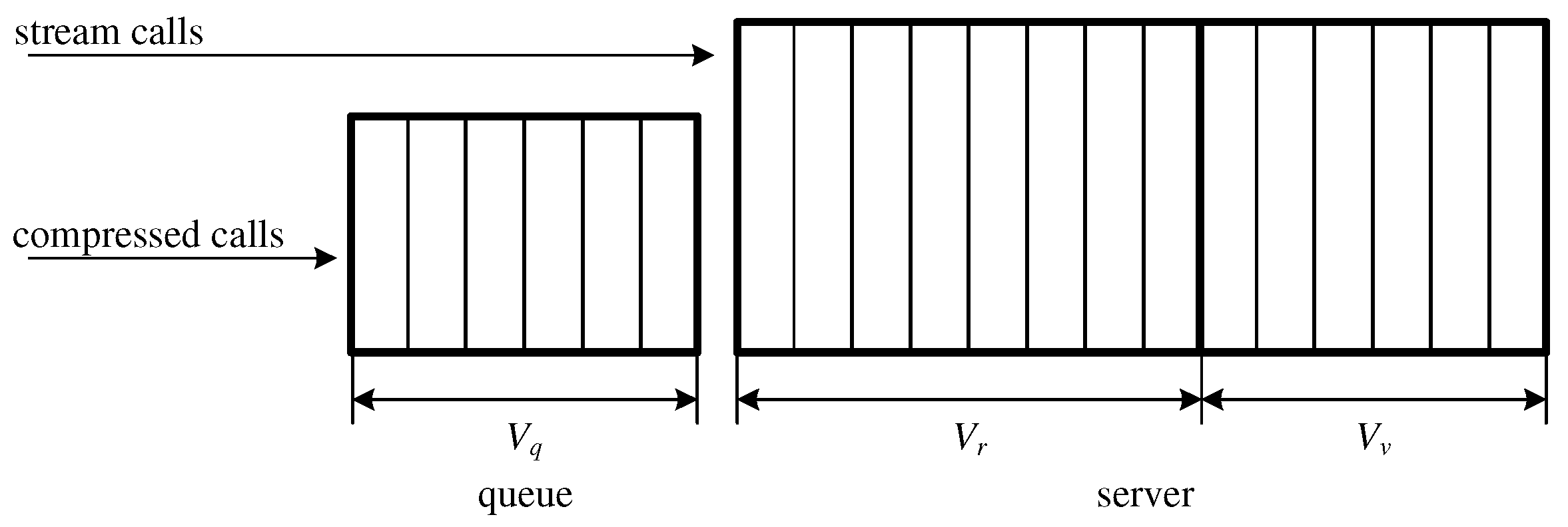
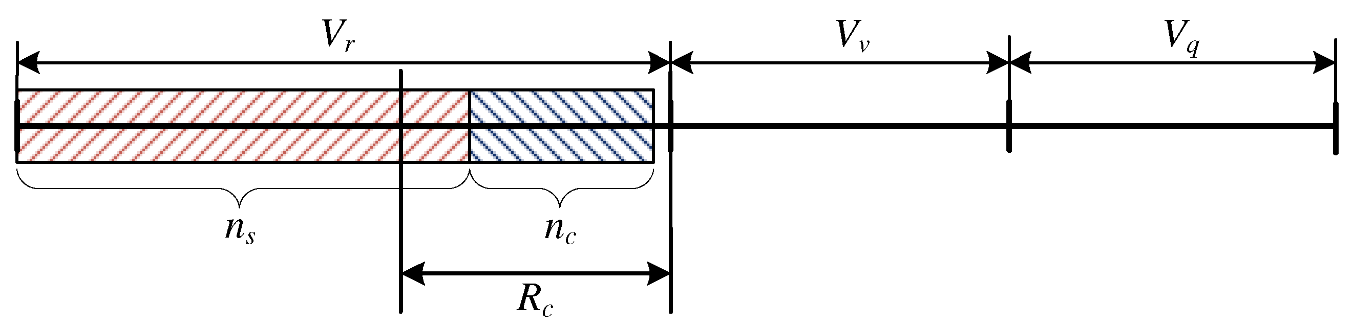
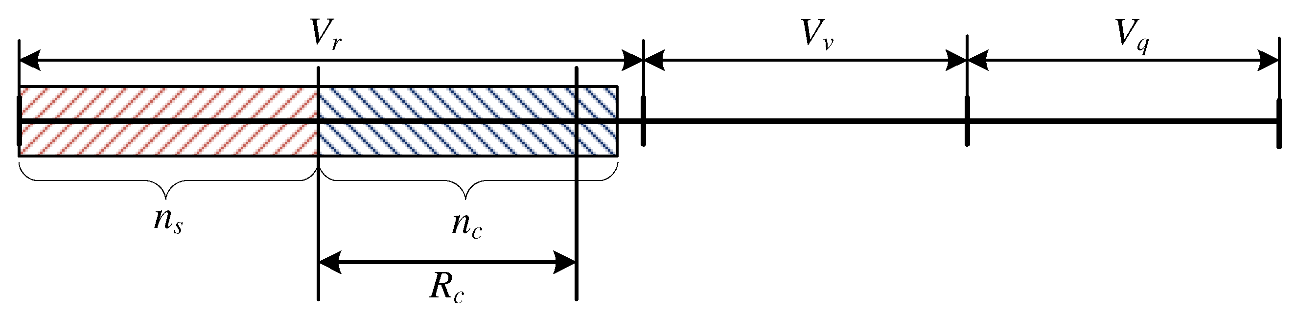
2.3. Structure and Working Principle of the Queuing System

The queuing system considered in this article consists of a server with the capacity of $V_r$ AUs and a buffer with the capacity of $V_q$ AUs. In the system, a portion of call flows can be subject to compression. This means that due to a decrease in the transmission rate (lower number of AUs allocated to a call for a service), more calls of this type can be serviced in the server. Data compression can also be represented by the additional virtual capacity $V_v$ introduced to the server, where additional calls will be serviced without any necessity to decrease the number of demanded AUs, while the maximum compression coefficient can be determined by the volume of the additional virtual capacity. This latter approach simplifies the analysis of the considered system at the service process level that takes place in the system. A simplified schematic diagram of this system is presented in Figure 2. For the calls that are subject to compression mechanism, the capacity of the server is $V_{rv}=V_r+V_v$, whereas for the uncompressed calls the capacity of the server is $V_r$. The accompanying assumption is that the calls that undergo compression mechanism cannot occupy more than $R_c$ AUs in the server, where $R_c<V_r$. The above assumption is crucial from the point of view of a determination of the compression coefficient (see: Section 3).

By knowing the structure of the system, we can consider the way in which new calls are admitted for service in the system. In the case of stream traffic (traffic that undergoes neither compression nor queuing), a new call of this type will be admitted for service if the server has free resources available that satisfy the requirements for this call. The accompanying assumption is that in order to ensure continuous service of the calls that are subject to compression, the stream calls can occupy $V_r-1$ AUs at the maximum. In addition, stream calls will not be admitted if the sum of demands of the calls that are being serviced in the server (stream and compressed calls) will be equal to $V_r+V_v$ AUs, even if the compressed calls occupy less than $V_r-1$ AUs. This limitation (constraint) results from the assumption of the limited compression in the system. In the case where the server has no available resources, the stream call will be lost.

In the case of the calls to be compressed in the server, i.e., elastic and adaptive calls, these calls can be placed in the queue. The assumption in the model is that in order to increase chances for service availability for stream calls, the operational constraint $R_c$ is introduced which defines the maximum number of AUs that these calls can occupy in the server. Hence, calls of this type will be admitted to the server if their call admittance does not exceed the amount of resource capacity available for this particular type of call. If a call cannot be admitted to the server, then it can be placed in the queue, provided the latter has enough free resources. If the queue has no free resources, the new compressed call is rejected. The accompanying assumption is that the queue in the considered system is serviced according to the FIFO (first in first out) discipline.

3. Analytical Model

Consider now a queuing system with the real capacity $V_r$ AUs and the capacity of the queue $V_q$ AUs. The system is offered $m_s$ stream traffic classes with the intensity ${\lambda }_{s,i}$, and $m_u$ traffic classes that undergo changes in the complete compression scheme with the intensity ${\lambda }_{c,i}$, where $c\in \{$e—the elastic call, and a—the adaptive call}. The demanded number of AUs for calls of the stream class and elastic or adaptive class will be denoted by $t_{u,i}$, where $u\in \{s$—denotes the stream call, e—the elastic call, and a—the adaptive call}. The call service process that takes place in the system can be considered either at the microstate or the macrostate level. The microstate is defined as a string of natural numbers that define the number of calls that are currently in the system $\left(X_{s,i},X_{c,i}\right)$, where $X_{s,i}$ denotes the number of calls of class i of the stream type that are currently in the system (serviced in the server, since calls of this type do not undergo queuing), $X_{c,i}$—defines the number of calls of class i that are subject to the compression in the system (in total, i.e., those calls that are serviced in the server and those that are in the queue), ($c\in \{e$—when the system is offered an elastic traffic class, and a—when the system is offered adaptive traffic}). The macrostate, in turn, defines the total number of AUs that are occupied by the calls serviced in the server and are waiting in the queue, with the division of the AUs between particular types of call classes taken into consideration. This means that the macrostate $\Omega (n_s,n_c)$ can be formally defined as the set of such microstates in which the total number of busy AUs in the system is equal to $n_s,n_c$, i.e.,

$$\begin{array}{ccc}\hfill \Omega (n_s,n_c)& =& \left\{\left(X_s,X_c\right):\sum _{i=1}^{m_s}{X}_{s,i}{t}_{s,i}=n_s\wedge \sum _{c\in \left\{e,a\right\}}\sum _{i=1}^{m_c}{X}_{c,i}{t}_{c,i}=n_c\right\}.\hfill \end{array}$$

(4)

3.1. Analysis of the Service Process at the Macrostate Level

Activation of the compression mechanism (scheme) is initiated when a newly arrived call of the elastic or adaptive traffic class cannot be admitted for service due to the lack of free resources. Activation of the compression mechanism in the case of elastic traffic classes results in a concurrent decrease in the number of demanded resources to such a value that will make admission of a new call possible, and also results in the accompanying extension of the service time. If the system is offered a traffic class of adaptive type, then compression is only followed by a decrease in the number of resources necessary for a connection to be set up. It should be stressed that the changes that result from the activation of the compression mechanism involve both the newly arrived calls and those that already undergo service, so that all calls in the system could be compressed in the same way. The proposed analytical model is based on the models [25,26], earlier proposed by the present authors. To simplify the mathematical analysis of systems with compression, defined in Section 2.3, the model employs the parameter of the virtual capacity, denoted as $V_v$, based on the description provided in [4]. This parameter makes it possible to adopt the following interpretation of the service process for calls of elastic and adaptive traffic classes: if the admission of a new call causes the number of resources occupied by calls that undergo service to exceed the real capacity $V_r$ but not to exceed the virtual capacity $V_v$, this call will be admitted for service; otherwise, the new call of elastic or adaptive traffic class is redirected to the queue. This will correspond to a situation in which calls of elastic and adaptive traffic are subject to compression (immediate decrease in the resources allocated for service). The call will be admitted to the queue as long as the queue has free resources that make this call possible for admission. The calls of the stream classes do not undergo compression. Another assumption in the system under consideration is that calls of this type are lost if there are no free resources necessary for the call to be serviced. In addition, to prevent the stream calls from being pushed out from the system by calls that undergo compression, a threshold $R_c$ ($R_c<V_r$) was introduced to the system. This threshold is defined as the maximum number of resources (AUs) that can be occupied in the server by calls that undergo compression. When this threshold is reached, calls of this type are placed in the queue, and when there are no free resources in the queue, the calls are lost. It should be stressed that the parameter $R_c$ does not mean that $R_c$ AUs for calls that undergo compression have been reserved in the server, but only that these calls can occupy $R_c$ AUs in the case where they are not occupied by calls that do not undergo compression. Note that according to the adopted method for servicing calls, the server can service this number of connections for which its occupancy does not exceed the virtual capacity. The introduced compression mechanism for elastic and adaptive calls causes the service stream in the states that do not exceed the real capacity to be equal to the total number of busy AUs in the system, whereas in all states in which the real capacity is exceeded it is equal to the real capacity of the system. Therefore, in the case of elastic and adaptive traffic, the number of demanded resources $t_{u,i}$ undergoes changes in the following way:

$$\begin{array}{c}\hfill {\displaystyle t_{u,i}\left(n_s,n_c\right)=\left\{\begin{array}{cc}{t}_{u,i},\hfill & \mathrm{when}\mathrm{compression}\mathrm{is}\mathrm{not}\mathrm{applied},\hfill \\ t_{u,i}·\xi (n_s,n_c),\hfill & \mathrm{when}\mathrm{compression}\mathrm{is}\mathrm{applied},\hfill \end{array}\right.}\end{array}$$

(5)

where $u\in \left\{e,a\right\}$, $\xi (n_s,n_c)$ is the compression coefficient (the occupancy areas of the system in which compression occurs, and its value is thoroughly determined further on in the article).

For the stream traffic classes, the number of demanded AUs in macrostate $\left(n_s,n_c\right)$ is constant and does not depend on the occupancy state of the system, i.e.,

$$\begin{array}{ccc}\hfill t_{s,i}\left(n_s,n_c\right)& =& t_{s,i},\mathrm{for}0\le n_s+n_c\le V_r+V_v+V_q.\hfill \end{array}$$

(6)

The average call service time for the stream and adaptive traffic classes does not change with the change in the state in which the system currently is, whereas the average call service time for the elastic traffic classes is shortened directly proportional to the decline in the number of demanded resources necessary for a connection to be set up. Therefore:

$$\begin{array}{c}\hfill {\displaystyle {\mu }_{e,i}\left(n_s,n_c\right)=\left\{\begin{array}{cc}{\mu }_{e,i},\hfill & \mathrm{when}\mathrm{compression}\mathrm{is}\mathrm{not}\mathrm{applied},\hfill \\ {\mu }_{e,i}·\xi (n_s,n_c),\hfill & \mathrm{when}\mathrm{compression}\mathrm{is}\mathrm{applied}\hfill \end{array}\right.}\end{array}$$

(7)

and

$$\begin{array}{ccc}\hfill {\mu }_{u,i}\left(n_s,n_c\right)& =& {\mu }_{u,i},\mathrm{for}0\le n_s+n_c\le V_r+V_v+V_q,\hfill \end{array}$$

(8)

where $u\in \left\{s,a\right\}$.

The average traffic offered by calls of class i of type u in macrostate $\left(n_s,n_c\right)$ expressed in AUs can be denoted by the symbol $A_{u,i}\left(n_s,n_c\right)$ and defined as the product of the average traffic intensity of offered traffic in a given macrostate ($a_{u,i}\left(n_s;n_c\right)$) and the number of demanded AUs ($t_{u,i}\left(n_s,n_c\right)$), i.e.,

$$A_{u,i}\left(n_s,n_c\right)=a_{u,i}\left(n_s,n_c\right)·t_{u,i}\left(n_s,n_c\right),$$

(9)

where $u\in \left\{s,e,a\right\}$.

Therefore, and on the basis of Formulae (5)–(8), we get:

$$\begin{array}{c}\hfill A_{u,i}\left(n_s,n_c\right)=A_{u,i},\end{array}$$

(10)

where $u\in \left\{s,e\right\}$ and

$$\begin{array}{c}\hfill A_{a,i}\left(n_s,n_c\right)=\left\{\begin{array}{cc}{A}_{a,i},\hfill & \mathrm{when}\mathrm{compression}\mathrm{is}\mathrm{not}\mathrm{applied},\hfill \\ A_{a,i}·\frac{1}{\xi (n_s,n_c)},\hfill & \mathrm{when}\mathrm{compression}\mathrm{is}\mathrm{applied}.\hfill \end{array}\right.\end{array}$$

(11)

Based on the derivations carried out in previous studies, one of which focused on a multi-service system with stream and elastic traffic [25], and another on a multi-service queuing system with elastic and adaptive traffic [26], and taking into account the properties of the service process in the system under consideration, the occupancy distribution in the queuing system where a mixture of stream, elastic, and adaptive traffic is offered can be expressed in the following recursive form:

$$\begin{array}{c}\hfill P(n_s,n_c)=\gamma (n_s,n_c)\left(\sum _{i=1}^{m_s}{A}_{s,i}P(n_s-t_{s,i},n_c)+\sum _{i=1}^{m_e}{A}_{e,i}P(n_s,n_c-t_{e,i})+\right.\\ \hfill \left.+\sum _{i=1}^{m_a}{A}_{a,i}\xi (n_s,n_c)P(n_s,n_c-t_{a,i})\right),\end{array}$$

(12)

where $\gamma (n_s,n_c)$ is the normalisation coefficient of the recurrent equation, whereas $\xi (n_s,n_c)$ is the compression coefficient.

Due to the specificity of the system under consideration, i.e., the concurrent service of call classes that undergo and do not undergo compression, the introduced constraint $R_c$ and the absence of queuing stream calls, to determine the occupancy distribution it is necessary to consider all possible dependencies between the number of AUs occupied by calls of individual types, since this has direct influence on the compression coefficient with which calls are compressed. These considerations were conducted in three areas:

• $0\le n_s+n_c\le V_r$,
• $V_r<n_s+n_c\le V_r+V_v$,
• $V_r+V_v<n_s+n_c\le V_r+V_v+V_q$.

3.1.1. Occupation of the System: $\mathbf{0}\le {\mathbf{n}}_{\mathbf{s}}+{\mathbf{n}}_{\mathbf{c}}\le {\mathbf{V}}_{\mathbf{r}}$

The first considered occupancy area is the one in which the total number of AUs occupied by serviced calls is lower than or equal to the real capacity $V_r$. Even though it seems that it is the simplest case, after taking into consideration the constraint (limitation) $R_c$, the following four cases were distinguished:

• $n_c\le R_c$ and $n_s\le V_r-R_c$,
• $n_c\le R_c$ and $n_s>V_r-R_c$,
• $R_c<n_c\le R_c+V_v$ and $n_s\le V_r-R_c$,
• $R_c+V_v<n_c\le R_c+V_v+V_q$ and $n_s\le V_r-R_c$.

Case Study: $n_c\le R_c$ and $n_s\le V_r-R_c$

In this particular case, the stream calls occupy $n_s$ AUs in total, whereas the calls that are subject to compression (elastic and adaptive) occupy in total $n_c$ AUs. Such an occupation state is presented in its simplified form in Figure 3, where the resources occupied by individual calls are marked cumulatively (this does not mean, of course, that the calls of individual types in the considered system have to occupy neighbouring resources of the system). As is noticeable, the stream calls occupy $n_s\le V_r-R_c$ AUs, which means that the calls that are compressed could potentially occupy $R_c$ AUs, but the number of occupied AUs by the calls of the same type is less than $R_c$. This in turn makes it possible to state that compression does not occur here, and that the queue is empty. The parameters $\gamma (n_s,n_c)$ and the compression coefficient are equal to $\xi (n_s,n_c)$:

$$\gamma (n_s,n_c)=\frac{1}{n_s+n_c}\wedge \xi (n_s,n_c)=1.$$

(13)

For this case of the occupancy, Equation (12) can be written in the following form:

$$\begin{array}{c}\hfill P(n_s,n_c)=\frac{1}{n_s+n_k}\left(\sum _{i=1}^{m_s}{A}_{s,i}P(n_s-t_{s,i},n_c)+\sum _{i=1}^{m_e}{A}_{e,i}P(n_s,n_c-t_{e,i})+\right.\\ \hfill \left.+\sum _{i=1}^{m_a}{A}_{a,i}P(n_s,n_c-t_{a,i}),\right).\end{array}$$

(14)

Case Study: $n_c\le R_c$ and $n_s>V_r-R_c$

This particular case of the occupancy in the considered system corresponds to the situation presented in Figure 4. Even though the number of serviced stream calls is so high that the calls that undergo compression cannot occupy $R_c$ AUs, there are fewer of them in the system than $V_r-n_s$, and as a result compression does not occur and the queue is empty. In this case, the parameters $\gamma$ and $\xi$ are described by Equation (13), whereas the occupancy distribution takes on the following form (14)—analogously as in the previous case.

Case Study: $R_c<n_c\le R_c+V_v$ and $n_s\le V_r-R_c$

This case of the occupancy corresponds to the situation in which the number of resources occupied by the stream calls is low enough that the calls that undergo compression can occupy $R_c$ AUs in the server (Figure 5). Since the total number of AUs demanded by these calls is higher than $R_c$, but fulfils the condition: $n_s+n_c\le V_r$, the elastic and adaptive calls will be compressed. The queue remains empty. This means that in the considered interval, compression does occur. Taking into consideration the dependence between the coefficients $\gamma$ and $\xi$ and the limitation $R_c$, the formulae that allow the values for this parameter to be determined can be written in the following form:

$$\gamma (n_s,n_c)=\frac{1}{n_s+R_c}\wedge \xi (n_s,n_c)=\frac{R_c}{n_c}.$$

(15)

Whereas the recursive dependence that makes it possible to determine the probability distribution will be written in the following form:

$$\begin{array}{c}\hfill P(n_s,n_c)=\frac{1}{n_s+R_c}\left(\sum _{i=1}^{m_s}{A}_{s,i}P(n_s-t_{s,i},n_c)+\sum _{i=1}^{m_e}{A}_{e,i}P(n_s,n_c-t_{e,i})+\right.\\ \hfill \left.+\sum _{i=1}^{m_a}{A}_{a,i}\frac{R_c}{n_c}P(n_s,n_c-t_{a,i}),\right).\end{array}$$

(16)

Case Study: $R_c+V_v<n_c\le R_c+V_v+V_q$ and $n_s\le V_r-R_c$

This is a particular case that takes place only when the relation between the parameters of the considered system and the number of occupied AUs by calls of individual types is as follows: $V_r-n_s>R_c+V_v$ i $V_r-n_s\le R_c+V_v+V_q$. In this case, the number of resources occupied by the calls that are subject to compression is so high that part of them is placed in the queue ($q(n_s,n_c)\ne 0$), despite the fact that the total occupancy of the system is lower than $n_s+n_c\le V_r$. This situation is illustrated in Figure 6. Formally, the resources occupied by the compressed calls should be marked in the corresponding capacity areas of the system (the virtual part $V_v$ and the queue $V_q$). However, in order to maintain continuity of the analysis of the service chain in the model, to determine whether calls are in the queue the relation between the parameters of the system ($V_r$, $V_v$, $V_q$) and the occupancy of the resources ($n_s$, $n_c$) must be taken into consideration. Similarly as in the previous considered cases, it is possible to determine the value of the parameter $\gamma$, the compression coefficient, and, additionally, the length of the queue (the number of busy resources in the queue):

$$\gamma (n_s,n_c)=\frac{1}{n_s+R_c}\wedge \xi (n_s,n_c)=\frac{R_c}{R_c+V_v}\wedge q(n_s,n_c)=n_c-R_c-V_v.$$

(17)

The occupancy distribution for this case can be determined from the following formula:

$$\begin{array}{c}\hfill P(n_s,n_c)=\frac{1}{n_s+R_c}\left(\sum _{i=1}^{m_s}{A}_{s,i}P(n_s-t_{s,i},n_c)+\sum _{i=1}^{m_e}{A}_{e,i}P(n_s,n_c-t_{e,i})+\right.\\ \hfill \left.+\sum _{i=1}^{m_a}{A}_{a,i}\frac{R_c}{R_c+V_v}P(n_s,n_c-t_{a,i}),\right).\end{array}$$

(18)

3.1.2. System Occupancy: ${\mathbf{V}}_{\mathbf{r}}\le {\mathbf{n}}_{\mathbf{s}}+{\mathbf{n}}_{\mathbf{c}}\le {\mathbf{V}}_{\mathbf{r}}+{\mathbf{V}}_{\mathbf{v}}$

Within this area, the assumption is that all calls occupy the resources that are higher than the real capacity $V_r$ and lower than the capacity of the server that results from the maximum compression, i.e., $V_r+V_v$. As in the earlier presented area, four cases were defined, in which the determination of the occupancy distribution of the resources in the system by calls of different types (compressed and not compressed) were considered. These included the following:

• $n_c\le R_c$ and $n_s>V_r-R_c$,
• $R_c<n_c\le R_c+V_v$ and $n_s\le V_r-R_c$,
• $R_c<n_c\le R_c+V_v$ and $n_s>V_r-R_c$,
• $R_c+V_v<n_c\le R_c+V_v+V_q$ and $n_s\le V_r-R_c$.

Case Study: $n_c\le R_c$ and $n_s>V_r-R_c$

In this case, the stream calls occupy such an amount of resources that the occupancy of $R_c$ units of the system capacity by compressed calls (elastic and adaptive) is not possible (Figure 7). The calls can occupy only $V_r-n_s$ AUs. Since the number of resources demanded by the compressed calls in all system satisfies: $V_r-N_s<n_c<V_r+V_w$, the queue is empty and the coefficients $\gamma$ and $\xi$ are, respectively, equal to:

$$\gamma (n_s,n_c)=\frac{1}{V_r}\wedge \xi (n_s,n_c)=\frac{V_r-n_s}{n_c}$$

(19)

The occupancy distributions in the system for the considered case of the occupancy of resources can be determined according to the following formula:

$$\begin{array}{c}\hfill P(n_s,n_c)=\frac{1}{V_r}\left(\sum _{i=1}^{m_s}{A}_{s,i}P(n_s-t_{s,i},n_c)+\sum _{i=1}^{m_e}{A}_{e,i}P(n_s,n_c-t_{e,i})+\right.\\ \hfill \left.+\sum _{i=1}^{m_a}{A}_{a,i}\frac{V_r-n_s}{n_c}P(n_s,n_c-t_{a,i}),\right).\end{array}$$

(20)

Case Study: $R_c<n_c\le R_c+V_v$ and $n_s\le V_r-R_c$

In this case of the occupancy of the considered queuing system, the calls that are subject to compression can occupy $R_c$ AUs in the server. Since their demands are higher than $R_c$ AUs, they undergo compression, which is presented in Figure 8. Since the demands of the compressed calls are lower than $R_c+V_v$, the queue is empty. The parameters $\gamma$ and $\xi$, as well as the occupancy distribution, can be determined on the basis of the following dependencies:

$$\gamma (n_s,n_c)=\frac{1}{n_s+R_c}\wedge \xi (n_s,n_c)=\frac{R_c}{n_c}$$

(21)

$$\begin{array}{c}\hfill P(n_s,n_c)=\frac{1}{n_s+R_c}\left(\sum _{i=1}^{m_s}{A}_{s,i}P(n_s-t_{s,i},n_c)+\sum _{i=1}^{m_e}{A}_{e,i}P(n_s,n_c-t_{e,i})+\right.\\ \hfill \left.+\sum _{i=1}^{m_a}{A}_{a,i}\frac{R_c}{n_c}P(n_s,n_c-t_{a,i}),\right).\end{array}$$

(22)

Case Study: $R_c<n_c\le R_c+V_v$ and $n_s>V_r-R_c$

In this case of the occupancy of the system, the number of occupied resources by the stream calls is so high that the calls that are subject to compression cannot occupy $R_c$ server resources (Figure 9). Since the demands of these calls are higher than $V_r-n_s$ but lower than $V_r-n_s+V_q$ AUs, the queue is empty but the elastic and adaptive calls undergo compression. By taking these dependencies into consideration, the coefficients $\gamma$ and $\xi$ can be determined in the following way:

$$\gamma (n_s,n_c)=\frac{1}{V_r}\wedge \xi (n_s,n_c)=\frac{V_r-n_s}{n_c}$$

(23)

The occupancy distribution takes on the following form:

$$\begin{array}{c}\hfill P(n_s,n_c)=\frac{1}{V_r}\left(\sum _{i=1}^{m_s}{A}_{s,i}P(n_s-t_{s,i},n_c)+\sum _{i=1}^{m_e}{A}_{e,i}P(n_s,n_c-t_{e,i})+\right.\\ \hfill \left.+\sum _{i=1}^{m_a}{A}_{a,i}\frac{V_r-n_s}{n_c}P(n_s,n_c-t_{a,i}),\right).\end{array}$$

(24)

Case Study: $R_c+V_v<n_c\le R_c+V_v+V_q$ and $n_s\le V_r-R_c$

In this case, the occupancy of the system is as follows: the number of AUs occupied by stream calls is lower than $V_r-R_c$, while the number of resources demanded by the compressed calls is so high that not all of the calls can be serviced, even in their compressed form. A number of calls have to be placed in the queue (Figure 10). In this case, the parameters $\gamma$, $\xi$ and the length of the queue can be determined in the following way:

$$\gamma (n_s,n_c)=\frac{1}{n_s+R_c}\wedge \xi (n_s,n_c)=\frac{R_c}{V_r+V_v-n_s}\wedge q(n_s,n_c)=n_c-R_c-V_v.$$

(25)

The occupancy distribution for the considered case can be determined from the following dependence:

$$\begin{array}{c}\hfill P(n_s,n_c)=\frac{1}{n_s+R_c}\left(\sum _{i=1}^{m_s}{A}_{s,i}P(n_s-t_{s,i},n_c)+\sum _{i=1}^{m_e}{A}_{e,i}P(n_s,n_c-t_{e,i})+\right.\\ \hfill \left.+\sum _{i=1}^{m_a}{A}_{a,i}\frac{R_c}{V_r+V_v-n_s}P(n_s,n_c-t_{a,i}),\right).\end{array}$$

(26)

3.1.3. Occupancy of the System: ${\mathbf{V}}_{\mathbf{r}}+{\mathbf{V}}_{\mathbf{v}}\le {\mathbf{n}}_{\mathbf{s}}+{\mathbf{n}}_{\mathbf{c}}\le {\mathbf{V}}_{\mathbf{r}}+{\mathbf{V}}_{\mathbf{v}}+{\mathbf{V}}_{\mathbf{q}}$

The assumption in this area is that calls collectively demand for their service resources that are higher than the capacity of the server which takes into account the maximum compression $V_r+V_v$, but lower than the capacity of the system that takes into account the capacity of the queue, i.e., $V_r+V_v+V_q$. Within this area, two cases were defined, in which the determination of the occupancy distribution of the resources of the system by calls of different types (compressed and non-compressed) was considered. These are as follows:

• $0<n_c\le R_c+V_v+V_q$ and $n_s>V_r-R_c$,
• $R_c+V_v<n_c\le R_c+V_v+V_q$ and $n_s\le V_r-R_c$.

The Case Study: $R_c<n_c\le R_c+V_v+V_q$ and $n_s>V_r-R_c$

In this case, the number of occupied resources by the stream calls does not allow the compressed calls to occupy $R_c$ AUs. On account of the number of the resources demanded for service by these calls, a number of them have to be placed in the queue, while the remainder undergo compression. A schematic diagram of the system occupancy for this particular case is presented in Figure 11. The parameters $\gamma$, $\xi$ and the length of the queue can be determined as follows:

$$\gamma (n_s,n_c)=\frac{1}{V_r}\wedge \xi (n_s,n_c)=\frac{V_r-n_s}{V_r+V_v-n_s}\wedge q(n_s,n_c)=n_c-V_r+n_s-V_v.$$

(27)

Taking the parameters $\gamma$ and $\xi$ into consideration, the state occupancy probability in the considered area takes on the following form:

$$\begin{array}{c}\hfill P(n_s,n_c)=\frac{1}{V_r}\left(\sum _{i=1}^{m_s}{A}_{s,i}P(n_s-t_{s,i},n_c)+\sum _{i=1}^{m_e}{A}_{e,i}P(n_s,n_c-t_{e,i})+\right.\\ \hfill \left.+\sum _{i=1}^{m_a}{A}_{a,i}\frac{V_r-n_c}{V_r+V_v-n_s}P(n_s,n_c-t_{a,i}),\right).\end{array}$$

(28)

The Case Study: $R_c+V_v<n_c\le R_c+V_v+V_q$ and $n_s\le V_r-R_c$

The considered case of the system occupancy is presented in Figure 12. The stream calls occupy not more than $V_r-R_c$ of the capacity resources of the system in the server. Because of the number of demanded resources by the calls that are to be compressed, they will also be placed in the queue, while the number of the resources occupied by the stream calls will have no effect on the compression coefficient. The parameters $\gamma$, $\xi$ and the length of the queue can be determined in the following way:

$$\gamma (n_s,n_c)=\frac{1}{n_s+R_c}\wedge \xi (n_s,n_c)=\frac{R_c}{R_c+V_v}\wedge q(n_s,n_c)=n_c-R_c-V_v.$$

(29)

Taking the parameters $\gamma$ and $\xi$ into consideration, the dependence that makes it possible to determine the occupancy distribution takes on the following form:

$$\begin{array}{c}\hfill P(n_s,n_c)=\frac{1}{n_s+R_c}\left(\sum _{i=1}^{m_s}{A}_{s,i}P(n_s-t_{s,i},n_c)+\sum _{i=1}^{m_e}{A}_{e,i}P(n_s,n_c-t_{e,i})+\right.\\ \hfill \left.+\sum _{i=1}^{m_a}{A}_{a,i}\frac{R_c}{R_c+V_v}P(n_s,n_c-t_{a,i})\right).\end{array}$$

(30)

To sum up the above considerations on the determination of the distribution in the presented system, you will find below tables in which the values of the parameters $\xi$ are juxtaposed (

Table 1. Value of the compression coefficient $\xi (n_s,n_c)$.

Area: $0\le {\mathit{n}}_{\mathit{s}}+{\mathit{n}}_{\mathit{c}}\le {\mathit{V}}_{\mathit{r}}$
	$n_s$	$n_s\le V_r-R_c$	$n_s>V_r-R_c$
$n_c$
$n_c\le R_c$		1	1
$R_c<n_c\le R_c+V_v$		$\frac{R_c}{n_c}$	—
$R_c+V_v<n_c\le R_c+V_v+V_q$		$\frac{R_c}{R_c+V_v}$	—
Area: $V_r<n_s+n_c\le V_r+V_v$
$n_c\le R_c$		—	$\frac{V_r-n_s}{n_c}$
$R_c<n_c\le R_c+V_v$		$\frac{R_c}{n_c}$	$\frac{V_r-n_s}{n_c}$
$R_c+V_v<n_c\le R_c+V_v+V_q$		$\frac{R_c}{R_c+V_v-n_s}$	—
Area: $V_r+V_v<n_s+n_c\le V_r+V_v+V_q$
$0<n_c\le R_c+V_v+V_q$		—	$\frac{V_r-n_s}{V_r+V_v-n_s}$
$R_c+V_v<n_c\le R_c+V_v+V_q$		$\frac{R_c}{R_c+V_v}$	—

) and $\gamma$ (

Table 2. Value of the coefficient $\gamma (n_s,n_c)$.

Area: $0\le {\mathit{n}}_{\mathit{s}}+{\mathit{n}}_{\mathit{c}}\le {\mathit{V}}_{\mathit{r}}$
	$n_s$	$n_s\le V_r-R_c$	$n_s>V_r-R_c$
$n_c$
$n_c\le R_c$		$\frac{1}{n_s+n_c}$	$\frac{1}{n_s+n_c}$
$R_c<n_c\le R_c+V_v$		$\frac{1}{n_s+R_c}$	—
$R_c+V_v<n_c\le R_c+V_v+V_q$		$\frac{1}{R_c}$	—
Area: $V_r<n_s+n_c\le V_r+V_v$
$n_c\le R_c$		—	$\frac{1}{V_r}$
$R_c<n_c\le R_c+V_v$		$\frac{1}{n_s+R_c}$	$\frac{1}{V_r}$
$R_c+V_v<n_c\le R_c+V_v+V_q$		$\frac{1}{n_s+R_c}$	—
Area: $V_r+V_v<n_s+n_c\le V_r+V_v+V_q$
$0<n_c\le R_c+V_v+V_q$		—	$\frac{1}{V_r}$
$R_c+V_v<n_c\le R_c+V_v+V_q$		$\frac{1}{n_s+R_c}$	—

) in dependence on the number of the resources occupied in the system by the stream calls and the compressed calls (elastic and adaptive):

3.2. System Characteristics

With the determined probability distribution $P(n_s,n_c)$, it was possible to determine the blocking probability in the system as well as the average lengths of the queues. To determine the blocking probability for calls of individual classes that belong to stream traffic or compressed stream, it is necessary to determine the space of the states that are blocking states for them. In the case of stream calls of class i, this set can be determined is the following way:

$${\Omega }_{E_{s,i}}=\{(n_s,n_c):(n_s<V_r-1)\wedge (n_s+t_{i,s}>C_r-1\vee n_s+n_c+t_{s,i}>V_r+V_v)\}$$

(31)

This set of states indicates that calls of this type will be rejected only when the number of AUs occupied by stream calls will be equal to $V_r-1$ or to the sum of the occupied resources by stream calls and compressed calls will be equal to $V_r+V_v$. For calls that are subject to compression and queuing when:

$${\Omega }_{E_{u,i}}=\{(n_s,n_c):(q(n_s,n_c)>0\wedge q(n_s,n_c)+t_{u,i}>V_q)\},$$

(32)

where $u=\{e,u\}$.

In this case, calls will be rejected if there is no space for them in the queue. The differences in the sets result from the way calls of particular types are serviced. We have to remember that in our system the stream calls are not placed in the queue and the compressed calls have guaranteed minimum resources (1 AU). Therefore, the blocking probability can be written in the following way:

$$E_{i,s}=\sum _{{\Omega }_{E_{i,s}}}P(n_s,n_c),$$

(33)

for stream calls, and:

$$E_{i,u}=\sum _{{\Omega }_{E_{i,u}}}P(n_s,n_c),$$

(34)

for calls that are subject to compression.

A very interesting property of the proposed model is its capacity to determine the total average length of the queue (here understood as the average number of occupied AUs in the queue) without the necessity of determining additional parameters: the average number of calls in the server and the average number of calls in the system. The average length of the queue can be determined using the observations made during the time when the parameters necessary to define the distribution were determined. In Section 3.1, besides the parameters $\xi$ and $\gamma$, the length of the queue in individual states is also determined, using the assumption that calls that are subject to compression will always be placed in the queue when their aggregate demand exceeds the service capacity of the server. In the case of a lack of free resources in the queue, calls will be rejected. The values of the lengths of the queues in individual occupancy areas of the considered system are summed up in

Table 3. Queue Length in States $n_s,n_c$ ($q(n_s,n_c)$).

Area: $0\le {\mathit{n}}_{\mathit{s}}+{\mathit{n}}_{\mathit{c}}\le {\mathit{V}}_{\mathit{r}}$
	$n_s$	$n_s\le V_r-R_c$	$n_s>V_r-R_c$
$n_c$
$n_c\le R_c$		0	0
$R_c<n_c\le R_c+V_v$		0	—
$R_c+V_v<n_c\le R_c+V_v+V_q$		$n_c-R_c-V_v$	—
Area: $V_r<n_s+n_c\le V_r+V_v$
$n_c\le R_c$		—	0
$R_c<n_c\le R_c+V_v$		0	0
$R_c+V_v<n_c\le R_c+V_v+V_q$		$n_c-R_c-V_v$	—
Area: $V_r+V_v<n_s+n_c\le V_r+V_v+V_q$
$0<n_c\le R_c+V_v+V_q$		—	$n_c-V_r+n_s-V_v$
$R_c+V_v<n_c\le R_c+V_v+V_q$		$n_c-R_c-V_v$	—

.

With the knowledge of the length of the queue in individual states, it is possible to determine the average number of busy AUs in the queue using the following formula:

$$q=\sum _{n_s=0}^{V_r}\sum _{n_c=0}^{R_c+V_v+V_q}q(n_s,n_c)P(n_s,n_c).$$

(35)

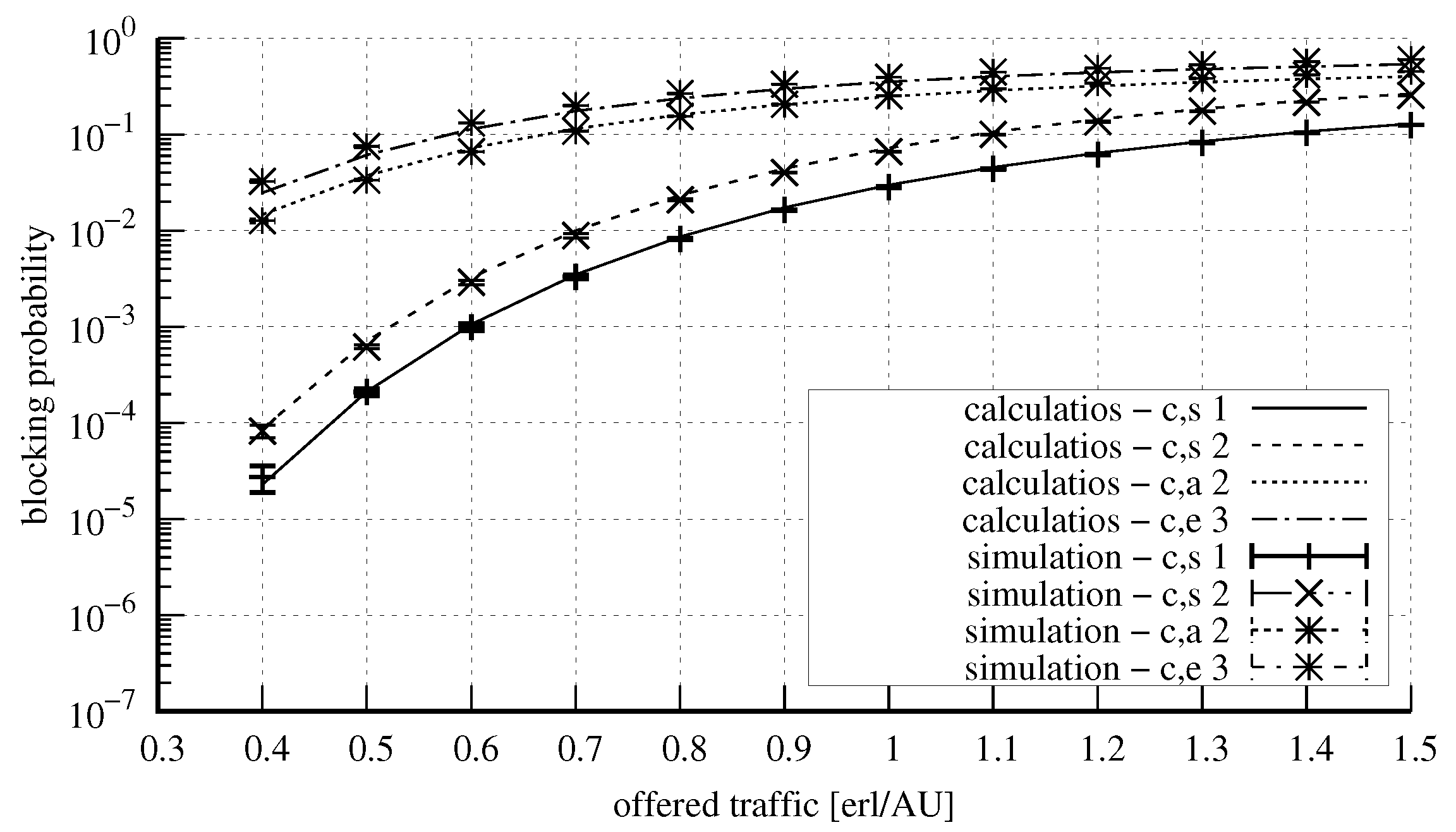
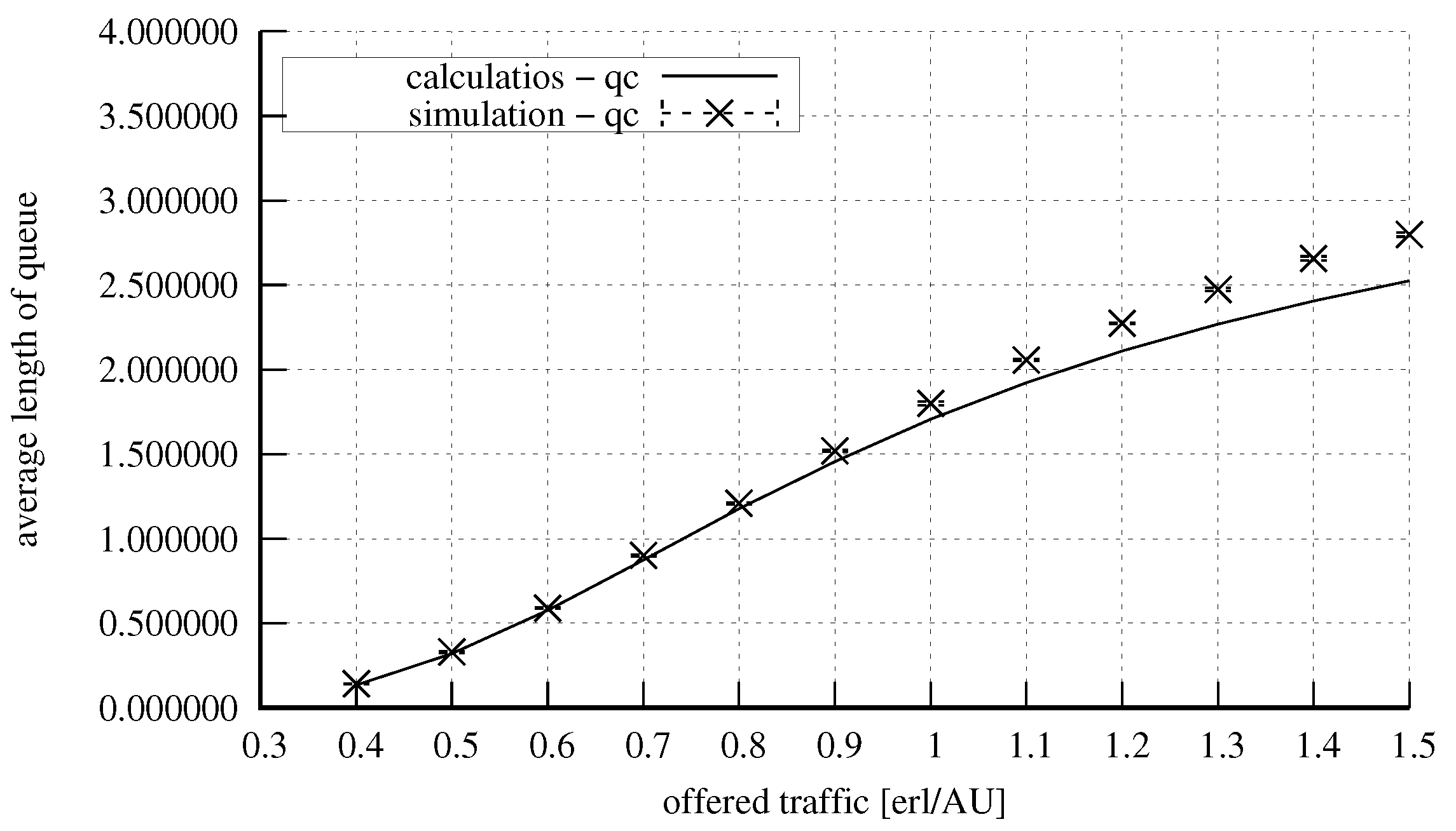
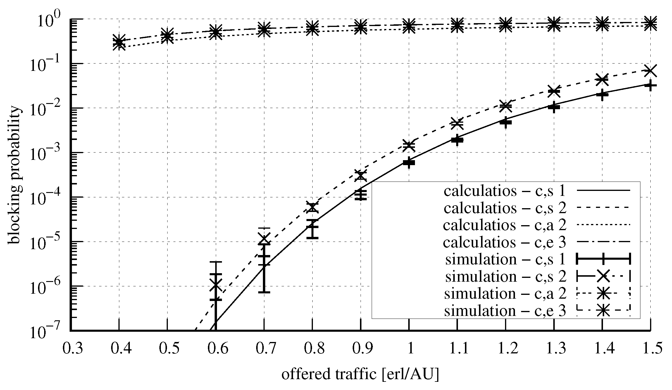
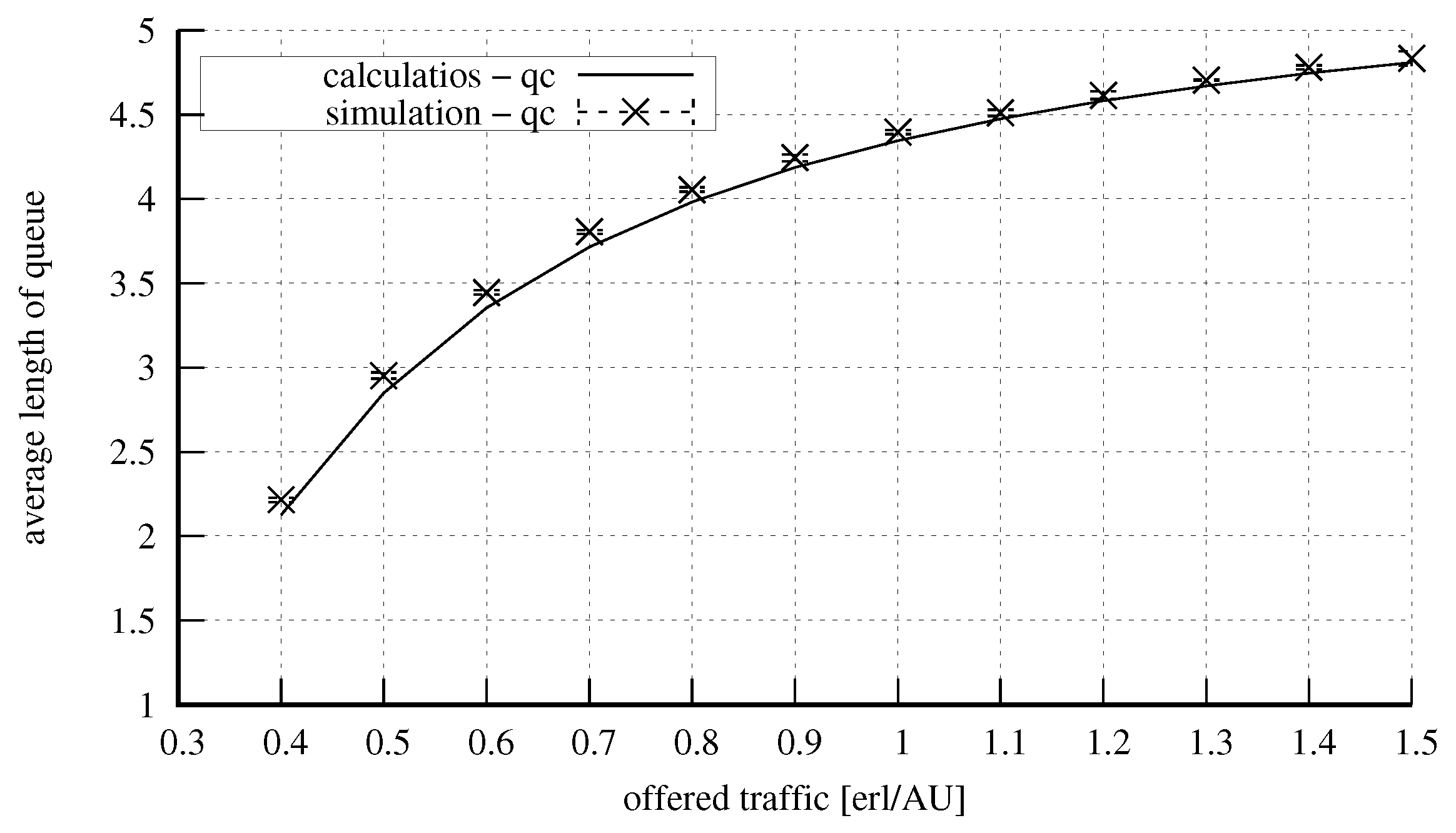
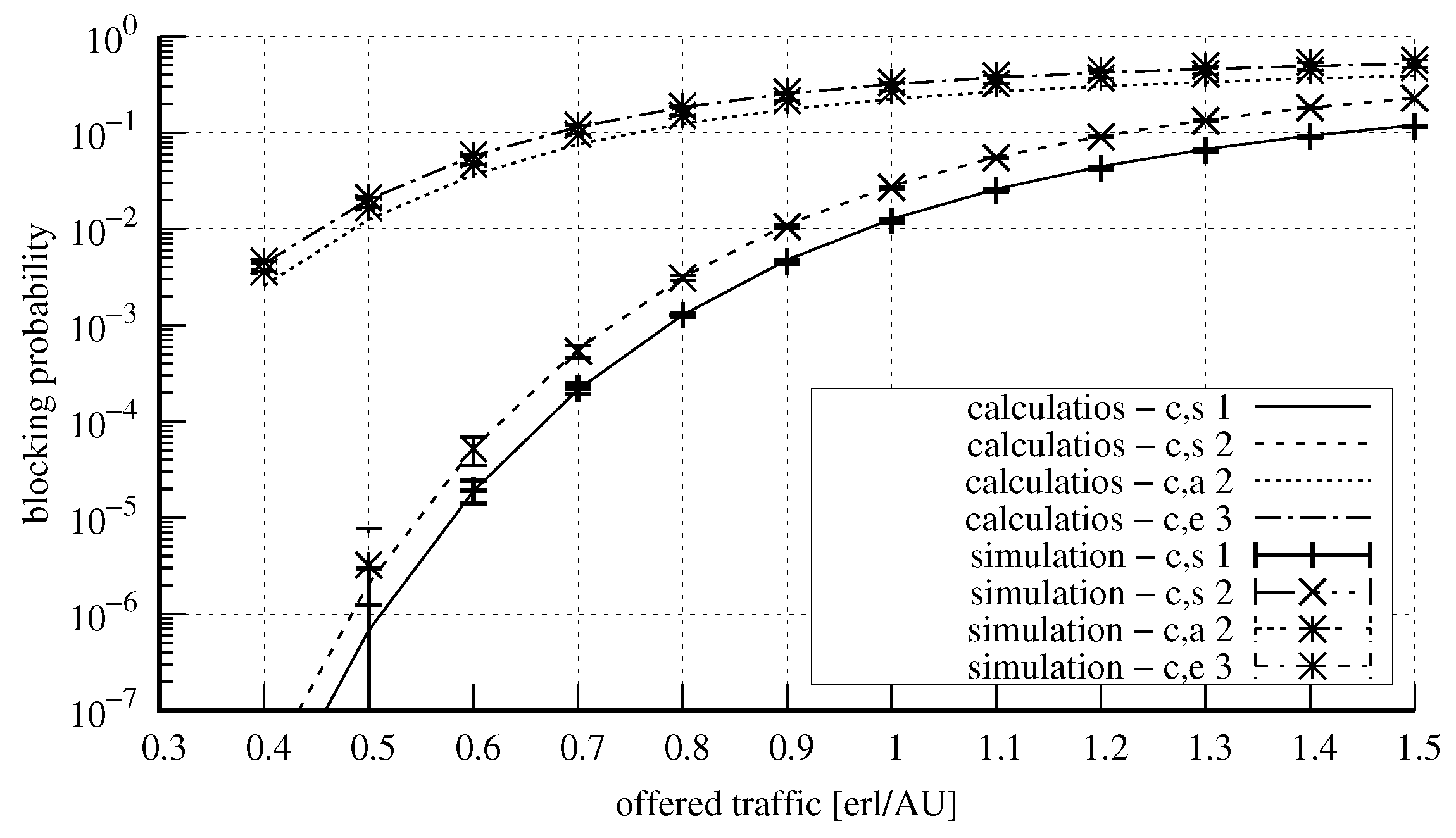
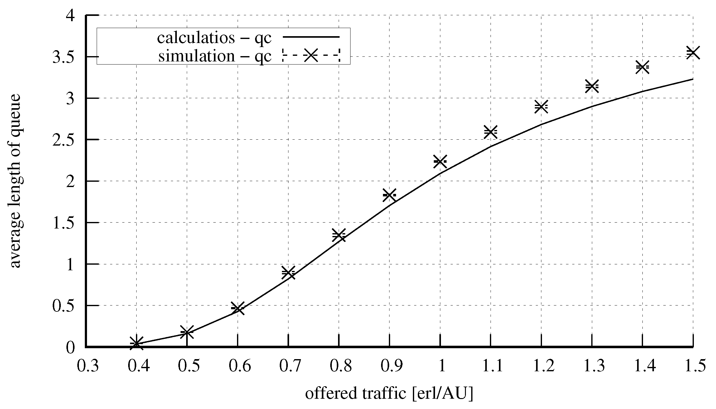
4. Numerical Results

The proposed analytical model is an approximation, wherein the actual service process in the system under consideration is substituted with a reversible Markov process. As a result, the results obtained by the model were compared with the results of a digital simulation. For this purpose, a simulator of the considered communications system was developed and implemented in the C++ language. To build the simulator, the event scheduling method [27] was used. The simulator allows the data necessary for the determination the system’s characteristics, such as the blocking probability or the average queue length for calls that undergo compression, to be collected and processed. All the results (blocking probability, average queue length) are presented as the function of offered traffic a for a single AU of the system:

$$a=\frac{{\sum }_{i=1}^m{A}_{i,u}}{V_r}.$$

(36)

Figure 13 and Figure 14 show the results obtained on the basis of the proposed model for a system with the parameters: $V_r$ = 10 AUs, $V_v$ = 5 AUs, and $V_q$ = 2 AUs. The constraint is that the number of the capacity units in the system that can be occupied in the server by calls that do not undergo compression $R_c$ is equal to 2 AUs. The system under consideration services three classes of calls: stream, elastic, and adaptive class. Calls of each of the classes demand for service a single unit of the system capacity: $t_{s,1}=t_{e,1}=t_{e,1}=1$ AU. Calls of each of the classes arrived in the system equally frequently, since the following proportion for offered traffic was assumed: $A_{s,1}:A_{e,1}:A_{a,1}=1:1:1$. Figure 13 shows the obtained values of the blocking probability, whereas Figure 14 presents the values of the total queue. As is easily noticeable, after the introduction of the constraints $R_c$ for compressed calls, their blocking probability is higher than that of the stream calls despite the fact that they demand identical amounts of resources for their service. The validation of the operation of the analytical model for small systems (low capacity in relation to call demands) was crucial as, frequently for such cases, approximate models are characterised by low accuracy. The presented results confirm high accuracy of the proposed model even for the case of the analysis of small systems.

Figure 15 and Figure 16 show the results for a system with the parameters $V_r$ = 20 AUs, $V_v$ = 8 AUs, $V_q$ = 5 AUs, $R_c$ = 5 AUs. The system was offered four traffic classes: two stream traffic classes that demanded 1 and 2 AUs, respectively, and two traffic classes of calls that were subject to compression: elastic that demanded 3 AUs for service, and adaptive that demanded 2 AUs.

Figure 17 and Figure 18 show the results for a system with the parameters $V_r$ = 50 AUs, $V_v$ = 10 AUs, $V_q$ = 6 AUs, and $R_c$ = 5 AUs. Four classes of calls were offered to the system, identically as in the case of the system presented above. Here, an increase in the capacity did not influence the accuracy of the model. Figure 19 and Figure 20, in turn, show the results for a system with the parameters exactly the same as in the previous system, but with the value of the parameter $R_c$ changed to the value of 15 AUs. An increase in the number of AUs that can be occupied in the server by calls that undergo compression resulted in the decrease in the blocking probability for these calls (at the expense of stream calls). The increase in the parameter $R_c$ also influenced the value of the average queue length, which was lower. Furthermore, let us note that as the parameter value of $R_c$ and the volume of offered traffic increase, there is a proportional increase in inaccuracies when estimating the average queue length.

5. Summary

This article proposes an analytical model of a communications and computer system, in which a number of constraints on the calls that were subject to compression, with the additional capacity of placing these calls in the queue, were introduced. The stream calls, due to their significance (e.g., control and management of the system) were not subject to queuing, so that they were not additionally delayed. Such an approach to the service of traffic streams of different types can be treated as a kind of a prioritisation mechanism. In the presented case, it is stream traffic that has higher priority. The model proposed in this article can be further extended to encompass scenarios where elastic or adaptive traffic is designed with higher priority. This aspect will be the subject of the research focus for the present authors in the near future. It is worth emphasising that, despite being an approximate model, the propose approach effectively serves its purpose in approximating systems with FIFO queue service discipline.

References

1. Xia, L.; Zhao, M.; Tian, Z. 5G Service Based Core Network Design. In Proceedings of the 2019 IEEE Wireless Communications and Networking Conference Workshop (WCNCW), Marrakech, Morocco, 15–18 April 2019; pp. 1–6. [Google Scholar] [CrossRef]
2. Agiwal, M.; Roy, A.; Saxena, N. Next Generation 5G Wireless Networks: A Comprehensive Survey. IEEE Commun. Surv. Tutor. 2016, 18, 1617–1655. [Google Scholar] [CrossRef]
3. Tataria, H.; Shafi, M.; Molisch, A.F.; Dohler, M.; Sjöland, H.; Tufvesson, F. 6G Wireless Systems: Vision, Requirements, Challenges, Insights, and Opportunities. Proc. IEEE 2021, 109, 1166–1199. [Google Scholar] [CrossRef]
4. Stamatelos, G.M.; Koukoulidis, V.N. Reservation-based Bandwidth Allocation in a Radio ATM Network. IEEE/ACM Trans. Netw. 1997, 5, 420–428. [Google Scholar] [CrossRef]
5. Rácz, S.; Gerő, B.P.; Fodor, G. Flow level performance analysis of a multi-service system supporting elastic and adaptive services. Perform. Eval. 2002, 49, 451–469. [Google Scholar] [CrossRef]
6. Bonald, T.; Virtamo, J. A recursive formula for multirate systems with elastic traffic. IEEE Commun. Lett. 2005, 9, 753–755. [Google Scholar] [CrossRef]
7. Logothetis, M.; Moscholios, I.D. Efficient Multirate Teletraffic Loss Models Beyond Erlang; John Wiley & Sons, Ltd.: Hoboken, NJ, USA, 2019. [Google Scholar] [CrossRef]
8. Hanczewski, S.; Stasiak, M.; Weissenberg, J. A Queueing Model of a Multi-Service System with State-Dependent Distribution of Resources for Each Class of Calls. IEICE Trans. Commun. 2014, E97-B, 1592–1605. [Google Scholar] [CrossRef]
9. Weissenberg, J.; Weissenberg, M. Model of a Queuing System with BPP Elastic and Adaptive Traffic. IEEE Access 2022, 10, 130771–130783. [Google Scholar] [CrossRef]
10. Ericsson. Ericsson Mobility Report; Technical Report; Ericsson: Hong Kong, China, 2021. [Google Scholar]
11. Głąbowski, M. Modelling of State-dependent Multi-rate Systems Carrying BPP Traffic. Ann. Telecommun. 2008, 63, 393–407. [Google Scholar] [CrossRef]
12. Głąbowski, M.; Sobieraj, M. Compression mechanism for multi-service switching networks with BPP traffic. In Proceedings of the 2010 7th International Symposium on Communication Systems, Networks & Digital Signal Processing (CSNDSP 2010), Newcastle Upon Tyne, UK, 21–23 July 2010; pp. 816–821. [Google Scholar] [CrossRef]
13. McArdle, C.; Tafani, D.; Barry, L.P. Overflow traffic moments in channel groups with Bernoulli-Poisson-Pascal (BPP) load. In Proceedings of the 2013 IEEE International Conference on Communications (ICC), Budapest, Hungary, 9–13 June 2013; pp. 2403–2408. [Google Scholar] [CrossRef]
14. Głąbowski, M.; Kmiecik, D.; Stasiak, M. On Increasing the Accuracy of Modeling Multi-Service Overflow Systems with Erlang-Engset-Pascal Streams. Electronics 2021, 10, 508. [Google Scholar] [CrossRef]
15. Liu, J.; Jiang, X.; Horiguchi, S. Recursive Formula for the Moments of Queue Length in the M/M/1 Queue. IEEE Commun. Lett. 2008, 12, 690–692. [Google Scholar] [CrossRef]
16. Isijola-Adakeja, O.A.; Ibe, O.C. M/M/1 Multiple Vacation Queueing Systems With Differentiated Vacations and Vacation Interruptions. IEEE Access 2014, 2, 1384–1395. [Google Scholar] [CrossRef]
17. Foruhandeh, M.; Tadayon, N.; Aïssa, S. Uplink Modeling of K-Tier Heterogeneous Networks: A Queuing Theory Approach. IEEE Commun. Lett. 2017, 21, 164–167. [Google Scholar] [CrossRef]
18. Czachorski, T. Queueing Models of Traffic Control and Performance Evaluation in Large Internet Topologies. In Proceedings of the 2018 IEEE 13th International Scientific and Technical Conference on Computer Sciences and Information Technologies (CSIT), Lviv, Ukraine, 11–14 September 2018; Volume 1, p. 1. [Google Scholar] [CrossRef]
19. Andonov, V.; Poryazov, S.; Otsetova, A.; Saranova, E. A Queue in Overall Telecommunication System with Quality of Service Guarantees. In Proceedings of the Future Access Enablers for Ubiquitous and Intelligent Infrastructures, Sofia, Bulgaria, 28–29 March 2019; Poulkov, V., Ed.; Springer International Publishing: Cham, Switzerland, 2019; pp. 243–262. [Google Scholar]
20. Chydzinski, A. Per-flow structure of losses in a finite-buffer queue. Appl. Math. Comput. 2022, 428, 127215. [Google Scholar] [CrossRef]
21. Cisco. Cisco Annual Internet Report (2018–2023); Technical Report; Cisco: San Jose, CA, USA, 2020. [Google Scholar]
22. Kelly, F.P.; Zachary, S.; Ziedins, I. (Eds.) Stochastic Networks: Theory and Applications, Notes on Effective Bandwidth; Oxford University Press: Oxford, UK, 1996; pp. 141–168. [Google Scholar]
23. Guerin, R.; Ahmadi, H.; Naghshineh, M. Equivalent capacity and its application to bandwidth allocation in high-speed networks. IEEE J. Sel. Areas Commun. 1991, 9, 968–981. [Google Scholar] [CrossRef]
24. Bonald, T.; Roberts, J.W. Internet and the Erlang Formula. SIGCOMM Comput. Commun. Rev. 2012, 42, 23–30. [Google Scholar] [CrossRef]
25. Hanczewski, S.; Stasiak, M.; Weissenberg, J. A Model of a System With Stream and Elastic Traffic. IEEE Access 2021, 9, 7789–7796. [Google Scholar] [CrossRef]
26. Hanczewski, S.; Stasiak, M.; Weissenberg, J. Queueing model of a multi-service system with elastic and adaptive traffic. Comput. Netw. 2018, 147, 146–161. [Google Scholar] [CrossRef]
27. Tyszer, J. Object-Oriented Computer Simulation of Discrete-Event Systems; Springer: New York, NY, USA, 2012. [Google Scholar]
Figure 1. Traffic types in communications and computer networks: (a) stream, (b) elastic, (c) adaptive.
Electronics 12 03601 g001
Figure 2. Schematic diagram of the structure of the considered queuing system.
Electronics 12 03601 g002
Figure 3. Schematic representation of the occupancy of the system within the interval n c R c and n s V r R c .
Electronics 12 03601 g003
Figure 4. Schematic diagram of the occupancy of the system within the interval n c R c and n s > V r R c .
Electronics 12 03601 g004
Figure 5. Schematic diagram of the occupancy within the interval R c < n c R c + V v and n s V r R c .
Electronics 12 03601 g005
Figure 6. Schematic diagram of the occupancy of the system within the interval R c + V v < n c R c + V v + V q and n s V r R c .
Electronics 12 03601 g006
Figure 7. Schematic diagram of the occupancy of the system within the interval n c R c and n s > V r R c .
Electronics 12 03601 g007
Figure 8. Schematic diagram of the occupancy of the system within the interval R c < n c R c + V v and n s V r R c .
Electronics 12 03601 g008
Figure 9. Schematic diagram of the occupancy of the system within the interval n c R c and n s > V r R c .
Electronics 12 03601 g009
Figure 10. Schematic diagram of the occupancy of the system within the interval R c + V v < n c R c + V v + V q and n s V r R c .
Electronics 12 03601 g010
Figure 11. Schematic diagram of the system within the interval R c < n c R c + V v + V q and n s > V r R c .
Electronics 12 03601 g011
Figure 12. Schematic diagram of the occupancy of the system within the interval R c + V v < n c R c + V v + V q and n s V r R c .
Electronics 12 03601 g012
Figure 13. Blocking probability in the system: V r = 10 AUs, V v = 5 AUs, V q = 2 AUs, R c = 2 AUs, t s , 1 = t e , 1 = t e , 1 = 1 AU.
Electronics 12 03601 g013
Figure 14. Average queue length in the system: V r = 10 AUs, V v = 5 AUs, V q = 2 AUs, R c = 2 AUs, t s , 1 = t e , 1 = t e , 1 = 1 AU.
Electronics 12 03601 g014
Figure 15. Blocking probability in the system: V r = 20 AUs, V v = 8 AUs, V q = 5 AUs, R c = 5 AUs, t s , 1 = 1 AU, t s , 2 = 2 AUs, t a , 1 = 2 AUs, t e , 1 = 3 AUs.
Electronics 12 03601 g015
Figure 16. Average queue length in the system: V r = 20 AUs, V v = 8 AUs, V q = 5 AUs, R c = 5 AUs, t s , 1 = 1 AU, t s , 2 = 2 AUs, t a , 1 = 2 AUs, t e , 1 = 3 AUs.
Electronics 12 03601 g016
Figure 17. Blocking probability in the system: V r = 50 AUs, V v = 10 AUs, V q = 6 AUs, R c = 5 AUs, t s , 1 = 1 AU, t s , 2 = 2 AUs, t a , 1 = 2 AUs, t e , 1 = 3 AUs.
Electronics 12 03601 g017
Figure 18. Average queue length in the system: V r = 50 AUs, V v = 10 AUs, V q = 6 AUs, R c = 5 AUs, t s , 1 = 1 AU, t s , 2 = 2 AUs, t a , 1 = 2 AUs, t e , 1 = 3 AUs.
Electronics 12 03601 g018
Figure 19. Blocking probability in the system: V r = 50 AUs, V v = 10 AUs, V q = 6 AUs, R c = 15 AUs, t s , 1 = 1 AU, t s , 2 = 2 AUs, t a , 1 = 2 AUs, t e , 1 = 3 AUs.
Electronics 12 03601 g019
Figure 20. Average queue length in the system: V r = 50 AUs, V v = 10 AUs, V q = 6 AUs, R c = 15 AUs, t s , 1 = 1 AU, t s , 2 = 2 AUs, t a , 1 = 2 AUs, t e , 1 = 3 AUs.
Electronics 12 03601 g020