1. Introduction
Multiple-Input and Multiple-Output (MIMO) technology has gradually matured after years of development and has become one of the key technologies used in intelligent communication [
1], and this technology enables communication systems to obtain higher transmission rates, system capacity, and spectral efficiency [
2]. In the field of wireless communication, because different types of services have different requirements for QoS (quality of service, QoS) latency and rate, and when considering resource allocation, it is necessary to take user service as the premise. Due to the limited spectrum resources and the demand for high-rate capacity, spectrum efficiency as a traditional performance index has long been widely studied [
3]. At the same time, with the need for the future development of green communication, the spectrum efficiency of the system is no longer blindly pursued; therefore, the optimization index of energy efficiency has emerged, and the improved energy efficiency means that the energy consumption of the system can be reduced [
4]. In the real environment, the RF link corresponding to each antenna in the MIMO system has a certain power consumption, and in the traditional MIMO system, due to the small number of antennas, the power consumption generated by this part of the RF link can usually be ignored. However, massive MIMO systems are equipped with a large number of antennas, resulting in circuit power consumption that cannot be ignored anymore [
5]. With an increasing number of antennas, the spectral efficiency of the system will continue to increase, while the energy efficiency will increase to a certain extent and then begin to decline, and the two restrict each other, presenting a contradictory relationship [
6], and it is difficult to achieve relative optimization at the same time. Therefore, for massive MIMO systems, the joint optimization of spectral efficiency and energy efficiency is still worth exploring.
Many scholars, both domestically and internationally, have conducted research on this topic. The research in [
7] proposes a power allocation method based on the maximum and minimum fairness criteria under massive MIMO systems, which maximizes the worst signal-to-noise ratio of all users and ensures the average performance for the users but does not consider the type of service and does not meet the QoS requirements of the users. The research conducted in [
8] studies the power allocation problem of massive MIMO systems and proposes a power allocation method using the asymptotic concave formation of the system sum rate, and the sum rate of the system increases with the increased number of antennas but ignores the index of spectral efficiency. The research in [
9] proposes a beam allocation and power optimization scheme, which is solved by expressing the problem of beam allocation and power optimization as a multivariate mixed integer nonlinear programming problem. This scheme has certain research value but does not consider the user’s QoS index. The research carried out in [
10] considers the QoS delay requirements of user services and the fairness of occupying wireless channels, and a power allocation strategy based on user expectations and pre-allocation is proposed to improve user satisfaction and fairness between users but the influence of channel status information is not considered. The research in [
11] uses power allocation to obtain optimal energy efficiency, but the default number of users meets the antenna restriction conditions, which is not in line with the access situation of users in practical applications. The research in [
12] obtains optimal energy efficiency through power allocation but does not add the limitation of the transmission power of the base station antenna, which will cause the power allocation to lose practical significance. The research in [
13] proposes a joint optimization design method for antenna selection and power distribution in massive MIMO systems. The research in [
14] optimizes energy efficiency under the constraints of spectral efficiency. The research in [
15] proposes an optimization algorithm for the energy efficiency of a massive MIMO system based on the particle swarm optimization algorithm, which takes the transmit power and the number of antennas in the system as the decision variables in the optimization, and uses the improved particle swarm optimization algorithm to solve it, which has certain advantages, but does not consider the factors of the number of users and user service. The research in [
16] takes the transmit power and the number of transmitting antennas as the decision variables to obtain the joint optimization problem of spectral efficiency and energy efficiency and then maps it to the NSGA-II algorithm for solving but does not consider the user-side situation, and there are few comparative experiments. With the continuous development of deep learning, neural networks have been applied to resource allocation, electromagnetism, and antenna fields. As described in document [
17], neural networks have been used in the field of communication resource allocation. Using a well-trained network to solve the resource allocation problem has very close performance and low computational complexity compared with traditional mathematics algorithms. The research in [
18] points out that neural networks in deep learning have made a breakthrough in terms of the antenna used for environmental sensing. The research in [
19] utilized deep neural networks for resource allocation among multiple users in MIMO systems. Firstly, the objective function is optimized based on the multi-objective sine c–sine algorithm. Secondly, the demand level of each user is identified, and a deep neural network algorithm is used to solve the problem, which to some extent, improves the system performance. However, the default number of users is less than the antenna limit, and there is no user scheduling, which is not in line with the actual situation.
According to the above analysis, there is little literature that has studied the joint optimization problem of energy efficiency and spectral efficiency based on the user service QoS guarantee. Therefore, the research in this paper is carried out in two steps, firstly, user scheduling is carried out under the condition of ensuring the QoS delay requirements of users, and the system capacity is maximized on the basis of equal power distribution. Then, the power of the scheduled users is re-distributed, the system energy efficiency is optimized on the basis of the refined QoS rate requirements, and the system capacity after adjusting the power is not lower than the system capacity in the first step of scheduling so as to establish a joint optimization problem, and finally, the Deep Q-Leaning Network (DQN) algorithm is to solve the problem.
The main contributions of this article are as follows: Before resource allocation, users are scheduled based on their business latency and channel state information to improve the satisfaction of different users. Based on the refinement of the QoS rate requirements, optimize system energy efficiency and ensure that the system capacity after power adjustment is not lower than the system capacity during the first step of scheduling in order to establish a joint optimization problem. Utilize the DQN algorithm to solve problems and improve system performance.
2. Problem Modeling
Firstly, a multi-user massive MIMO system model is established, and the block diagonalization precoding method is used under this system model equivalent to the multi-user system as a single-user system in order to eliminate the interference of other users [
20]. Then, based on the average power allocation, user scheduling is carried out based on service QoS delay requirements and channel status, and the system capacity is calculated. Then, under the requirements of ensuring the upper and lower limits of transmitter power and QoS rate, the selected users are reallocated to optimize the system’s energy efficiency, the system capacity in the scheduling stage is corrected, and the objective function of the spectrum efficiency and energy efficiency joint optimization is established to achieve a compromise between the two.
2.1. System Model
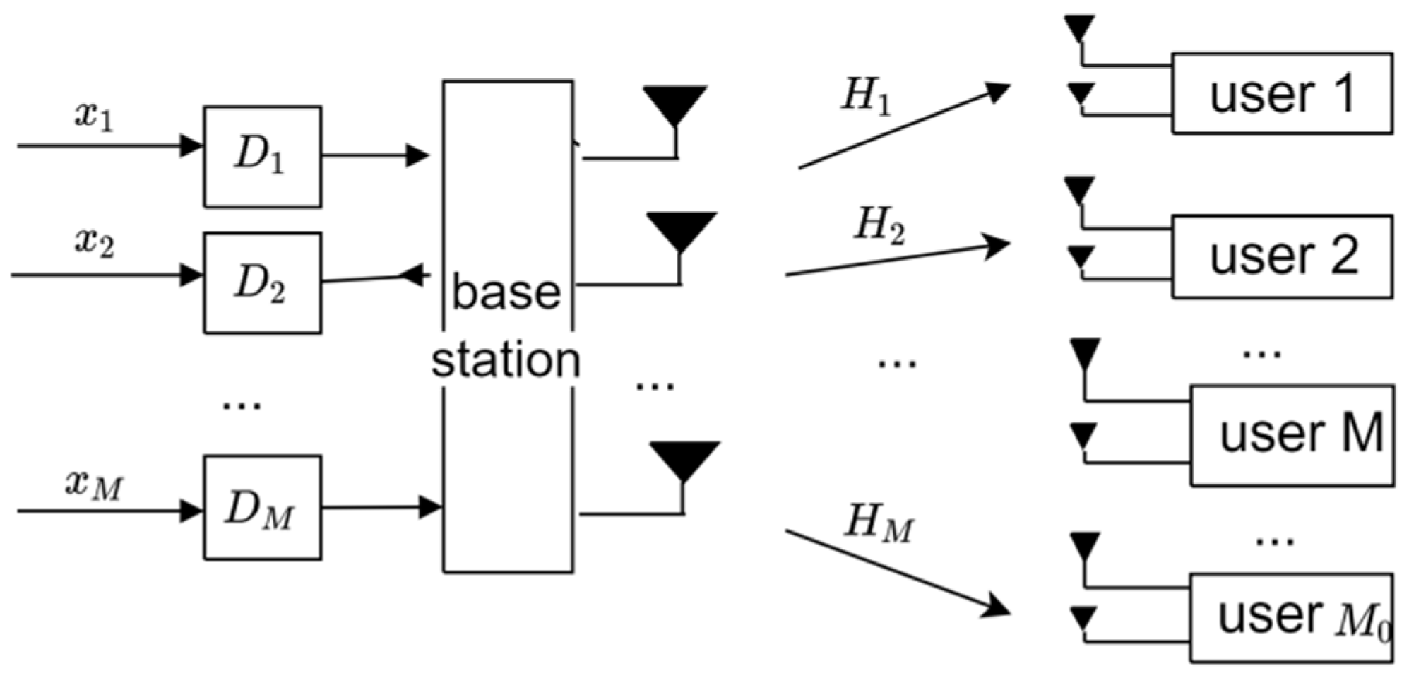
This paper takes the downlink of a multi-user massive MIMO system as the background, assuming that the base station has
transmitting antennas and
users, and if the number of receiving antennas for the
mth user is
, the base station can support
M users to communicate at the same time in each scheduling time slot. The system model is shown in
Figure 1.
In a massive MIMO system, in order to improve the spectral efficiency of the system, all users are allowed to reuse the same time–frequency resources. In this way, each user will receive signals from other users in addition to receiving the signals they need, resulting in inter-user interference. Therefore, in the transmitter end of the downlink system, it is generally necessary to use precoding technology to preprocess the transmitted signal in order to increase the signal-to-noise ratio, thereby accelerating the data transmission rate and improving the performance of the entire system. In this paper, block diagonalization precoding is used to decompose the downstream channel matrix of a multi-user MIMO system into a block diagonalized form, which is equivalent to multiple single-user MIMO systems that do not interfere with each other, eliminating interference from other users. The equivalent channel model is shown in
Figure 2.
Assuming that the channel state information of the base station transmitter is known,
represents the transmit signal vector of the
mth user, and
represents the received signal vector of the
mth user, and then there are:
where
represents the signal required by the
mth user,
represents interference from other users, and
represents additive white Gaussian noise in the
mth user channel.
represents the complex Gaussian random channel matrix for the
mth bit, and
represents the precoded matrix for the
mth use. Block diagonalization is applied to find the pre-coded matrix,
, so that the interference from other users is zero, and for the
mth user, the matrix consisting of the channel matrix of the other users is as follows:
where
is the
-dimensional full-rank matrix. Decomposing
by singular value yields the following:
where
is the unitary matrix of order
,
is a diagonal matrix composed of
non-zero singular values of
,
is the conjugate transpose matrix of
, consisting of
and
,
is composed of right singular vectors corresponding to
non-zero singular values of
, and
is composed of right singular vectors corresponding to
zero singular values.
According to the unitary matrix property:
; therefore, Equation (3) can be written as follows:
Multiplying the left and right of formula (6) together gives:
According to (7), for the mth user, can eliminate the interference of other users, and in order to solve the equation system, needs to be satisfied, which is the use of the block diagonalization method to remove multi-user interference on the user scheduling scheme constraints; that is, the maximum number of simultaneous communication users M limit.
Further, let
and perform singular value decomposition to obtain:
where
is an
-dimensional matrix,
is a
-dimensional unitary matrix,
is a
-dimensional matrix,
is a diagonal matrix composed of
non-zero singular values, and
is composed of right singular vectors corresponding to
non-zero singular values of
.
Take the block diagonalized precoded matrix of
and substitute
into Equation (1) to obtain the following:
where
is the equivalent channel matrix. Substituting Equation (8) into (9) yields:
Multiply
on both sides to obtain:
where
and
are the diagonal matrices in which the diagonal elements are not zero and the other elements are all zero. Let the diagonal element of
be
and let
to have
.
Block diagonalized precoding equates multi-user channels to multiple independent single-user channels, which in turn can be equivalent to multiple parallel channels. At this point, the data rate
of the
mth user after bandwidth normalization can be expressed as follows:
where
represents the signal power of the
mth user on the kth parallel channel, the diagonal element
of
represents the channel fading coefficient, and
represents the power of additive white Gaussian noise.
2.2. User Scheduling
In practical applications, due to the burstiness of users, the number of users accessing the system will be greater than the limit of the number of antennas at the base station end; therefore, user scheduling is required first in resource allocation, and M users are selected in each scheduling time slot to maximize system throughput while ensuring user service QoS requirements.
This article discusses four types of user services: conversational class, streaming class, interaction class, and background class. The conversational class focuses on real-time requirements, and the most critical QoS indicator is latency, which is very severe and will cause the session to fail to proceed normally; therefore, latency is listed as an important indicator affecting the conversational class. The streaming class does not require interactions between two users, and data are only transmitted in one direction; therefore, the service has certain real-time requirements but is not as strict as the conversational class. Compared with the previous two, the delay requirements of the interactive class are not high. The background class basically has no hard requirements in terms of delay. Therefore, this article takes latency as the indicator of the QoS requirements in the user scheduling stage and specifies that the delay requirement is the maximum time that data are waiting in the queue.
Table 1 shows the rate and delay requirements of the four services.
Among them, the conversation class pays the most attention to real-time experiences, and the most critical QoS indicator is delay, which will cause the session to not continue normally when the delay is very serious. In the streaming class, data are transmitted in one direction, which has certain real-time requirements, but it is not as strict as that of the conversational class. Compared with the previous two, the delay requirements of the interactive class are not so strict. The background class only cares about whether the data are transmitted correctly and almost do not require delay. In summary, this chapter takes delay as the QoS metric in the user scheduling stage and specifies that the delay requirement is the maximum time that data wait in the queue.
The number of antennas used in real life is not enough for users to use according to the above business characteristics, which for delay requirements, often need user scheduling in order to be achieved, assuming that users only use one service in a certain time slot, in the user scheduling stage, consider the user’s service delay and channel status, set the number of user waiting time slots to
, the maximum number of waiting time slots to
, set a scheduling cycle to t, and the delay requirement is expressed by the maximum number of waiting cycles:
. When scheduling, first dispatch the user services that
is about to reach or exceed
, and if all the users who meet the conditions have been accessed but there are still antennas left, the channel state information of the user is considered. The user scheduling process is shown in
Figure 3:
As can be seen from the above flowchart, the specific execution method of user scheduling is:
Step 1: Initialize all user collections, set the unchecked collection to and the selected collection to .
Step 2: Determine the number of waiting time slots for each service , and if , select User M. Update the user collection, selected, unchecked.
Step 3: If the number of selected users exceeds the antenna limit, it ends. Otherwise, select User that satisfies . At this point , update the user collection , .
Step 4: Iterate through the remaining user collection N. For each user s in N, define and calculate the capacity of set : . In set N, if a user satisfies , let at this time. Otherwise, end the algorithm and then update and update user collection , .
Step 5: Repeat step 4 to finally update the user collection.
2.3. Joint Optimization Function Establishment
After user scheduling, it can ensure the delay requirements of the user’s business. However, this stage is performed under the circumstances of average power distribution. Therefore, it is necessary to redistribute power and optimize the system capacity obtained during the scheduling phase. To ensure the normal progress of the business, the lowest limit of
is set to set the rate. Similarly, in order to avoid waste of resources, try not to exceed the user m rate upper limit of
. Therefore, the rate of user
m is limited as follows:
The total rate of all selected users is:
The optimization objective of this article is not only to maximize the throughput of the scheduled user set but also to consider energy efficiency as an important indicator in this article. Assuming that
is the upper limit of the transmitting power of the
i-root antenna, the power
limit of the launch antenna is as follows:
In summary, the total launch power of the base station can be expressed as follows:
among them,
is the efficiency of the base station power amplifier.
is the power consumption of the circuit component, which is a fixed value, defining the energy efficiency
as follows:
Therefore, the optimization proposed in this article is as follows:
It can be observed that if
is maximized, the greater the power consumption, the worse the energy efficiency
. The two restrict each other and are difficult to optimize at the same time. The total capacity
after power redistribution should be greater than the total capacity at average allocation in order to be meaningful. Therefore, this article uses the main objective method to transform the problem, with
as the main optimization objective and
as the constraint, thus transforming the problem into:
3. Solving the Combination Optimization Problem Based on DQN Algorithm
The joint optimization problem proposed above is the problem of NP-difficulty non-convex optimization. It is more complicated to use traditional methods when solving this problem. Therefore, for this decision-making problem, this article uses the DQN model in deep Q learning to solve this problem. Among them, the neural network of the Q value function is selected from the deep neural network of the full connection. In the above resource allocation, define each user as an intelligent agent. At the moment of , the user observes the current status of the environment , then use the strategy to adopt action from the allowable set of action set and obtain a reward , and then obtain the status and reward in the next moment.
Status collection: set as the maximum waiting cycle of the user, and record the status corresponding to the
-transmission time of the learning process as follows:
Action collection: Define actions as selecting users and allocating power and record the action corresponding to the
t-th transmission time interval of the learning process as
. Among them,
is a dual variable, and its value is determined by using
:
To reduce the set of actions, simplify the actions as follows:
Instantaneous reward is defined as energy efficiency, and the instantaneous reward for executing action
in state
is recorded as follows:
Cumulative reward: the cumulative reward for executing action
in state
is defined as the state action value function
and expressed as incremental updates:
among them,
represents the current value function of action
executed in state
at time
, and
represents the maximum value function corresponding to various actions
taken by time
in state
.
represents the learning rate, usually taken as a very small value.
represents the discount factor related to the future.
The objective value function of executing action
in state
is denoted as the sum of the maximum
Q value of the reward and the discount in the next state:
The DQN model adopts a dual network structure, which records the current
Q value and the target
Q value separately. The purpose of training the neural network is to reduce the difference between the current
Q value and the target
Q value by minimizing the loss function. The loss function
is defined as follows:
The solution model based on DQN is as
Figure 4, after each action selection, the intelligent agent will store the state, action, rewards obtained, and the state of the next time in the experience pool. When the experience pool is full, the network starts to update. The reward and the next moment’s state are used to calculate the
Q value, and the target
Q value is calculated from the
Q value, and then the loss function value is calculated until convergence.
It can be seen from the above that the pseudocode for solving the above optimization problem with DQN is as follows (Algorithm 1):
| Algorithm 1: DQN |
Initialize experience playback pool and capacity ;
Initialize parameter of the current Q-value network ;
Initialize parameter of target Q-value network , i.e., ;
for episode = 1, M do
Randomly select initial state ;
for t = 1, T do
if random < do
Select actions based on the strategy and randomly select action with probability ;
else
Select action
end if
Execute action , observe reward and the next state ;
Store memory, store in experience playback pool ;
Batch extract sample data from to train the current Q-value network;
Using the function, the parameter is updated through the gradient back propagation of the neural network;
Copy and update the target Q-value network parameter every T round of cycling;
end for
end for |
5. Conclusions
Aiming at the problem of low throughput and energy efficiency in large-scale MIMO systems due to the mutual constraints between energy efficiency and spectral efficiency and the lack of consideration of user service QoS and the rate of the upper and lower limits in resource allocation, a method based on the combined optimization of spectrum and energy resources under QoS guarantees is proposed. This method is divided into two steps. First, greedy algorithms are used to schedule users based on their latency requirements. Then, a joint optimization problem model is established by setting upper and lower rate requirements for the selected users. Finally, the DQN method is used to solve the problem. The simulation results show that the algorithm proposed in this article can ensure user QoS requirements and improve user satisfaction while also improving throughput and energy efficiency to a certain extent.
This article focuses on the downlink of multi-user massive MIMO systems. The next step is to focus on the multi-objective optimization problem of the uplink of massive MIMO systems. In the future, more resource allocation issues will be considered, including power, bandwidth, antenna number, etc. This joint resource allocation problem is very useful for future communication users.


