Accelerating the Response of Self-Driving Control by Using Rapid Object Detection and Steering Angle Prediction

Abstract

A vision-based autonomous driving system can usually fuse information about object detection and steering angle prediction for safe self-driving through real-time recognition of the environment around the car. If an autonomous driving system cannot respond fast to driving control appropriately, it will cause high-risk problems with regard to severe car accidents from self-driving. Therefore, this study introduced GhostConv to the YOLOv4-tiny model for rapid object detection, denoted LW-YOLOv4-tiny, and the ResNet18 model for rapid steering angle prediction LW-ResNet18. As per the results, LW-YOLOv4-tiny can achieve the highest execution speed by frames per second, 56.1, and LW-ResNet18 can obtain the lowest prediction loss by mean-square error, 0.0683. Compared with other integrations, the proposed approach can achieve the best performance indicator, 2.4658, showing the fastest response to driving control in self-driving.

1. Introduction

In recent years, the self-driving system has become a trend worldwide. This study imitates the advanced driver assistance system developed by Tesla to develop a vision-based autonomous driving system in a model car. Therefore, this study will focus on real-time object detection and image recognition through image sensors to realize vision-based autonomous driving. At the same time, the car moves on the road, which is a highly complex task.

Applying AI visual algorithms to the autonomous driving system can fuse rapid object detection and steering angle prediction information to accomplish imminent response and achieve safe driving. Regarding object detection, the AI visual algorithm YOLOv4-tiny [1], a lightweight version of YOLOv4 [2], can detect objects precisely in front of a self-driving car, including vehicles and traffic signs. Similarly, another AI visual algorithm ResNet18 [3], a variant of ResNet models [4], can predict the steering angle precisely in front of a self-driving car, including multi-lanes and intersections. If an autonomous driving system cannot respond fast to driving control appropriately, it will cause high-risk problems with regard to severe car accidents from self-driving. However, YOLOv4-tiny and ResNet18 models cannot run rapidly enough to respond quickly to self-driving driving control. Therefore, this study seeks to identify a lightweight version of YOLOv4-tiny that can run on GPUs in real-time to fulfill rapid object detection. In addition, this study also needed to find a lightweight version of ResNet18 to accomplish rapid steering angle prediction. According to the improved models above, the autonomous driving system will integrate rapid object detection and steering angle prediction to control driving quickly and safely.

Regarding the imitation of a self-driving car running on a road in an urban area, a planar road map simulates a scenario of real roads to allow a model car called Nvidia JetRacer [5] to drive autonomously on it, where a model car is installed with seven cameras surrounding it and equipped with the embedded Nvidia Jetson Nano [6] to execute AI visual computing. The model car will self-drive based on the road map, including two-way lanes and intersections, where we placed vital traffic signs, such as various speed limits, traffic lights, directions, and stop signs, aside from the lanes, to simulate the scenario of autonomous driving like a natural road mesh. We collected a large amount of image data from the above-mentioned experimental environment to give AI visual models supervised learning and use the TensorRT [7] inference engine to simultaneously fuse real-time rapid object detection and steering angle prediction. This study will evaluate a variety of integration systems and give a comparison of their performance. As a result, the main contribution of this study is proposing an approach that can achieve the best performance and showing the fastest response of driving control in self-driving.

2. Related Work

2.1. Literature Review

Bojarski et al. [8] proposed a convolutional neural network that maps the raw pixels of a single front camera directly to steering commands. With minimal human training data, the system automatically learns to drive the vehicle on local roads and highways with and without lane markings, such as by detecting natural road features and using the steering angles captured from actual human beings driving as training signals. Duong et al. [9] developed a navigation method for autonomous vehicles. A convolutional neural network on the UDACITY platform trained and simulated the unmanned vehicle model. They installed three cameras in front of the vehicle to track and collect data in the left, right, and center directions.

Do et al. [10] showed a prototype of an autonomous vehicle by using deep neural networks based on a monocular vision on a Raspberry Pi. The authors focused on finding a model that uses deep neural networks to directly map raw input images to predicted steering angles as the output. Jain et al. [11] gave a working model of an autonomous vehicle capable of driving from one location to another on different tracks, such as curved, straight, and straight-back curved tracks. They installed a camera on top of the car, and the Raspberry Pi feeds the image from the convolutional neural network, which then predicts the left and right directions. Seth et al. [12] presented the demonstration and implementation of a self-driving car based on convolutional neural networks. The vehicle used a 1/10 scale RC car as the primary basis for system control, with the camera as the primary input. For the computing platform, they used a Raspberry Pi 4 development board to enhance the function and installed an ultrasonic sensor in the system for obstacle avoidance.

Omrane et al. [13] built an autonomous RC car that was controlled by using an artificial neural network (ANN). It describes the theory behind neural networks and self-driving cars and how to design a camera to test and evaluate algorithm capabilities with footage as the only input. Simmons et al. [14] practiced an end-to-end learning method that enables small, low-cost, remote-controlled cars to follow lanes in austere indoor environments. Training deep neural networks (DNNs) and convolutional neural networks (CNNs) can map raw imagery from foreground shots to steering and speed commands (right, left, forward, backward). The concept proposed by Karni et al. [15] used a remote control car as a basis to build an autonomous miniature car. As mentioned above, image processing can achieve the goals. They used vision-based neural networks from deep learning to accomplish the self-driving model.

2.2. Object Detection Model YOLOv4-Tiny

Based on the architecture of YOLOv3, the architecture of YOLOv4 has significantly improved the accuracy and speed of object detection [16]. Furthermore, the YOLOv4-tiny is a lightweight model of YOLOv4, which can speed up the inference of object detection. The purpose of adopting the lightweight model is to effectively realize the inference in a small-sized embedded platform with a limited computation capacity. In other words, YOLOv4-tiny can implement real-time object detection without any delay of inference in the embedded platform.

The architecture of the YOLOv4-tiny model consists of three parts: backbone, neck, and head (prediction), as shown in Figure 1. In the backbone, there are three CSP_Blocks in which the Cross Stage Partial Network (CSPNet) architecture can reduce the amount of computing and enhance the feature extraction capability. This part can implement better object detection in the neck through feature fusion. In the prediction, the prediction part outputs feature maps of three sizes. Small-size feature maps are suitable for detecting large-size objects because small-size feature maps can better represent the overall object features of large-size objects. Conversely, large-sized feature maps are suitable for detecting small objects because large-sized feature maps can easily observe and detect small objects.

Figure 1. YOLOv4-tiny architecture. (Different color means different function performed in a single block).

The excellent performance of YOLOv4 benefits a few novel techniques: image data enhancement Mosaic [2] by using Cutmix [17], DropBlock [18] regularization, Class Label Smoothing [19], Mish [20] activation function, CSPNet [21] architecture, CIOU [22] Loss function, Cross Mini-Batch Normalization (CmBN) [2], Convolutional Block Attention Module (CBAM) [23], and others.

2.3. Object Detection Model YOLOv5

YOLOv5 [24] uses many novel skills, such as the image data enhancement method of the Mosaic, adaptive image scaling, and Focus structure. Using these skills can significantly improve the capability of object detection. Mosaic can significantly improve the detected effect of YOLOv5 in small objects by splicing and randomly scaling the picture. Object detection uses image scaling to adjust the length and width of the input image during inference. It calculates the scaling ratio based on the long side, which can effectively reduce the length of the short side to reduce the amount of computing and improve the inference speed. The Focus structure increases the amount of computing for slicing and combining so that the feature map will not lose feature information due to compression. The YOLOv5 model consists of input, backbone, neck, and prediction, as shown in Figure 2.

Figure 2. YOLOv5 architecture. (Different color means different function performed in a single block).

In the backbone, the Focus block is responsible for down-sampling, and its slicing and combination can prevent the loss of feature information. The middle part includes a series of convolutional layers and BottleneckCSP layers for feature extraction. Adding the CSPNet architecture can reduce the amount of computing and enhance the feature extraction capability. Finally, the SPP layer [25] strengthens the feature expression ability and avoids the poor detection effect caused by the significant difference in object size. This part can implement better object detection in the neck through feature fusion. In the prediction, the prediction layer of YOLOv5 outputs the same feature maps of three sizes as the YOLOV4-tiny mentioned above. Small-size feature maps are suitable for detecting large-size objects, and conversely, large-size feature maps are suitable for detecting small objects.

2.4. Object Detection Model YOLOv7

YOLOv7 [26] optimizes the model architecture and training process. YOLOv7 gives an extended, efficient layer aggregation network and model scaling skills in model architecture. In the training process, YOLOv7 adopts a model re-parameterized skill to replace the original module and uses a dynamic label assignment strategy to assign labels to different output layers. Figure 3 shows the architecture of the traditional YOLOv7 model, consisting of input, backbone, neck, and prediction.

Figure 3. YOLOv7 architecture. (Different color means different function performed in a single block).

In the backbone, the CBS layer is the basic convolutional unit, including convolution, batch normalization, and SiLU activation functions. The ELAN layer consists of multiple CBS structures, and its feature map output consists of three parts. Here, the feature map is equally divided into two groups by channel. Then, the first group implements five convolution operations to obtain the first part, the second group implements one convolution operation to obtain the second part, and the third part is composed of the results of the first convolution and the third convolution of the first group. The MP layer divides the feature map into two groups. The first group executes maximum pooling to extract more critical information, and the second group conducts convolution to extract the feature information. Finally, combining two groups obtains the result.

In the neck, the feature map output of the SPPCSPC layer consists of two parts. Here, the feature map is divided into two groups by channel. The first group implements three convolution operations and then three consecutive maximum poolings to separate three sets of different sizes of feature maps to acquire multiple features. After combining multiple features, it implements a second convolution operation to obtain the first part. The second group implements a convolution operation to obtain the second part. The CUC layer is the basic unit of feature map combination, including convolution, up-sampling, and combining feature maps. The REP layer is a novel concept that uses the skill of structural reparameterization to adjust the structure in inference to improve the performance of the model. With three parts, the REP layer can obtain the feature map output during the training process. The first and the second parts implement a convolution operation and batch normalization. The third part only implements batch normalization. The inference of REP only retains the second part of the structure by using structural reparameterization, reducing computing resources, and improving model performance.

In the prediction, the prediction layer of YOLOv7 outputs the same feature maps of three sizes as the YOLOV4-tiny mentioned above and YOLOv5. Small-size feature maps are suitable for detecting large-size objects, and conversely, large-size feature maps are suitable for detecting small objects.

2.5. Steering Angle Prediction Model ResNet18

As the network depth of the CNN model increases, the model accuracy for image recognition does not constantly improve, and this problem is obviously not caused by overfitting. The deepened network not only causes the test error to become higher, but its training error is even higher. The deeper networks will come up with a vanishing/exploding gradient problem, which hinders the convergence of the network in the training phase, called the degradation problem [4]. Batch normalization [27] can alleviate this problem to a certain extent, but it is still not enough to meet the needs.

ResNet models [4] can solve this degradation problem. ResNet has five versions: Res18, Res34, Res50, Res101, and Res152. Each version of ResNet includes three parts: input, output, and intermediate convolutions, where the intermediate convolutions consist of four stages from stage #1 to stage #4. Although there are many variants of ResNet, they all follow the above-mentioned structural characteristics. The difference between the networks lies mainly in the differences in the block parameters and the number of intermediate convolutions. To achieve the fastest response time for the inference, we use ResNet18 for image recognition, as shown in Figure 4.

Figure 4. ResNet18 architecture. (Different color means different function performed in a single block).

3. Method

3.1. Model Car and Planar Road Map

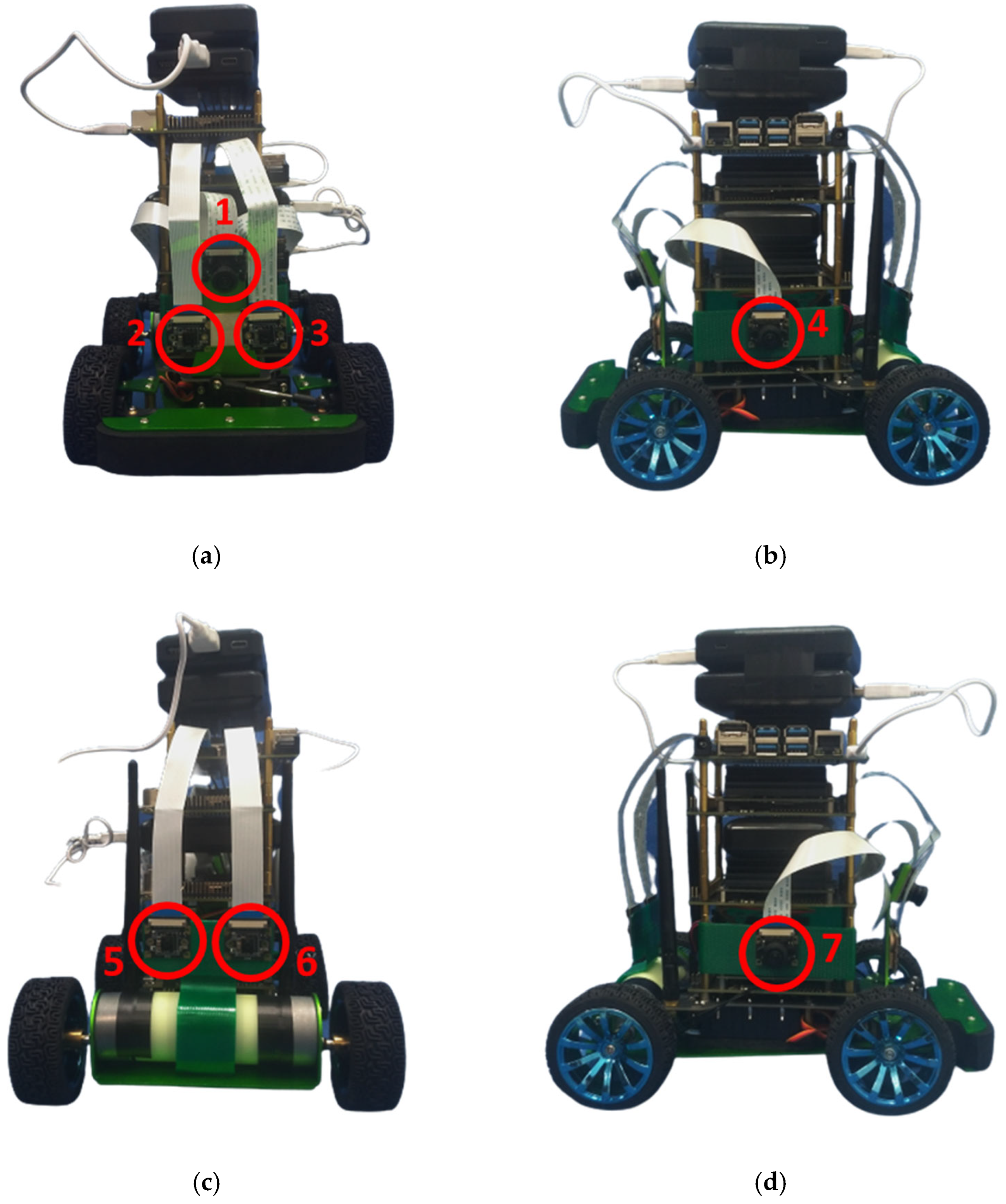
The boxed battery located at the base of JetRacer supplies power to Jetson Nano and the motor inside JetRacer. In addition, the mobile power attached to JetRacer supplies power to the other Jetson Nanos. Servo and DC gear motors control the rear wheels, which can drive JetRacer. Tie rods fix the front wheels, and the other parts control the steering of the car. We installed seven onboard cameras around JetRacer, forming a 360-degree panoramic view through which to look around and perceive environmental information, as shown in Figure 5. The autonomous driving system calls the drive motor, and the steering programs execute the driving JetRacer through the library. The control of the motor speed and steering degree of JetRacer ranges from −1 to 1. The autonomous driving system performed the object detection and steering angle prediction and then sent the results back to JetRacer. In such a way, JetRacer can decide whether to move forward or backward and turn left or right.

Figure 5. Onboard cameras surrounding a JetRacer. (a) Three front cameras indicated #1, #2, and #3. (b) Left camera indicated #4. (c) Two rear cameras indicated #5 and #6. (d) Right camera indicated #7.

We designed a scenario that let JetRacers self-drive on a planar road map that simulates real roads for the simulation and test of autonomous driving, as shown in Figure 6. Furthermore, this study also produced small-size traffic signs such as speed limit signs, turn signs, stop signs, and traffic lights. JetRacer can drive on a planar road map and follow traffic signal rules, as shown in Figure 7.

Figure 6. Planar road map where color yellow represents the lines to distinguish lanes in different directions and color white stands for the lines to indicate road edge.

Figure 7. Planar road map with traffic signs.

3.2. Data Collection

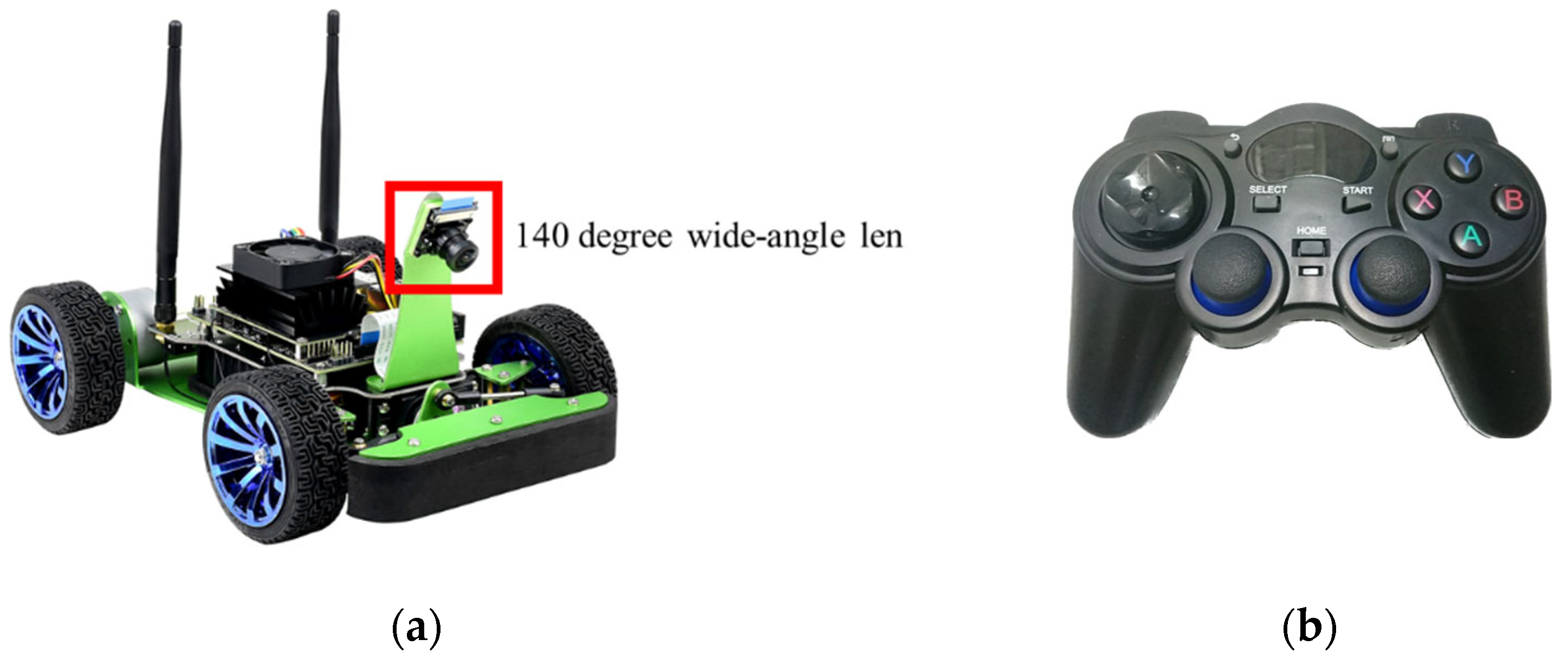
The controller operated JetRacer to move on the road map in small increments for data collection. By collecting images from different angles at each point on the path, the autonomous driving system can learn how to correct the lane. The wide-angle camera mounted on the front of JetRacer has a 140-degree viewing range. Data collection from this camera can help JetRacer move along the route more accurately, as shown in Figure 8. This study needed to collect two datasets. The first dataset contains various objects, such as vehicles and different traffic signs, and the second includes the routes of the planar road map. To implement the object detection task, we needed to manually label the first dataset, as shown in Figure 9.

Figure 8. Data collection using the front-end camera and handle controller. (a) Front-end camera; (b) handle controller.

Figure 9. Traffic signs and roads in the training phase. (a) Speed limit sign. (b) Stop sign. (c) Traffic light.

3.3. Rapid Response Time from Using LW-YOLOv4-Tiny and LW-ResNet18 Models

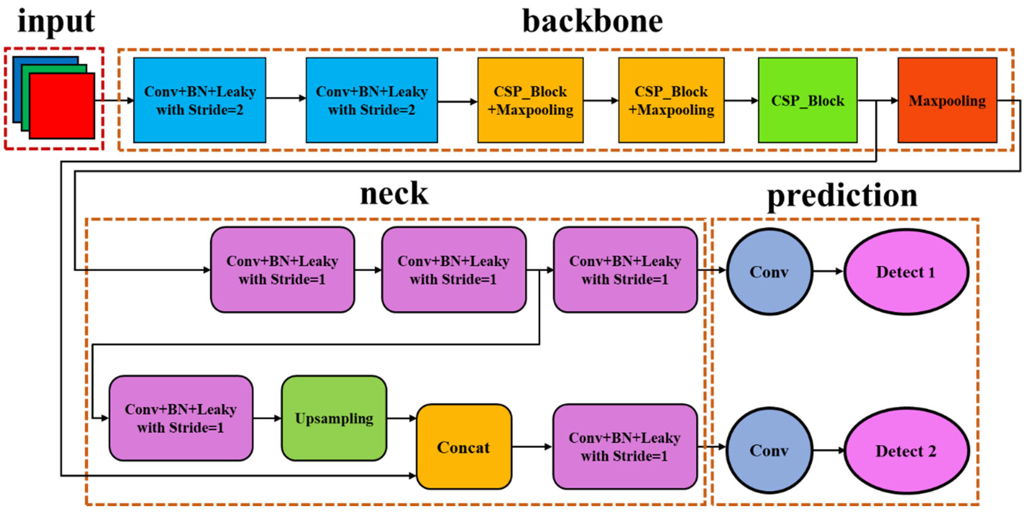
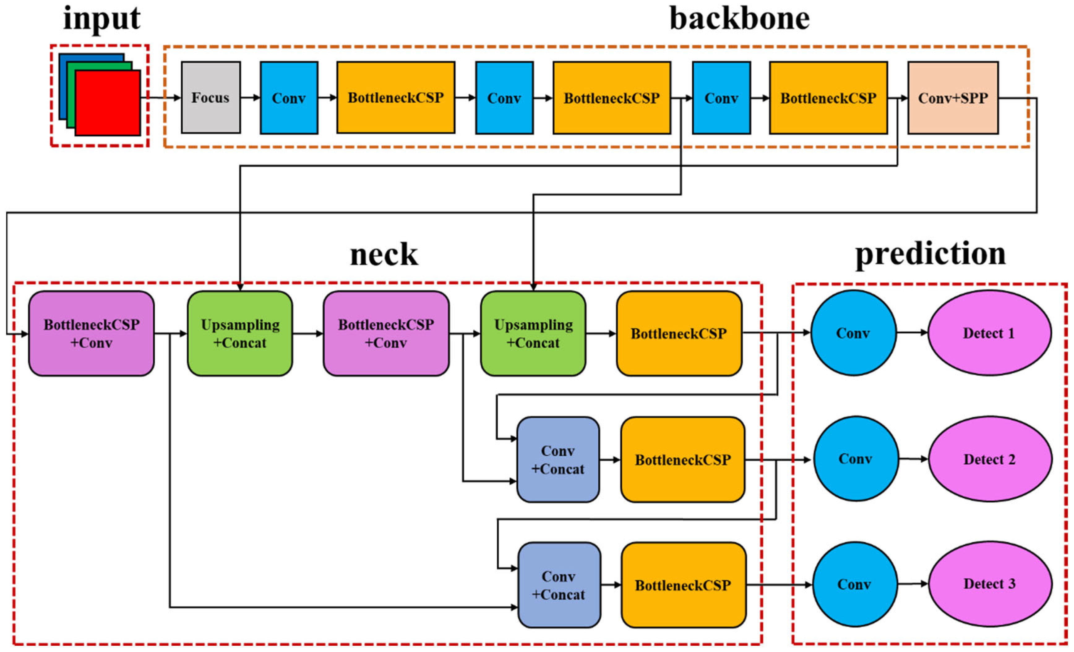
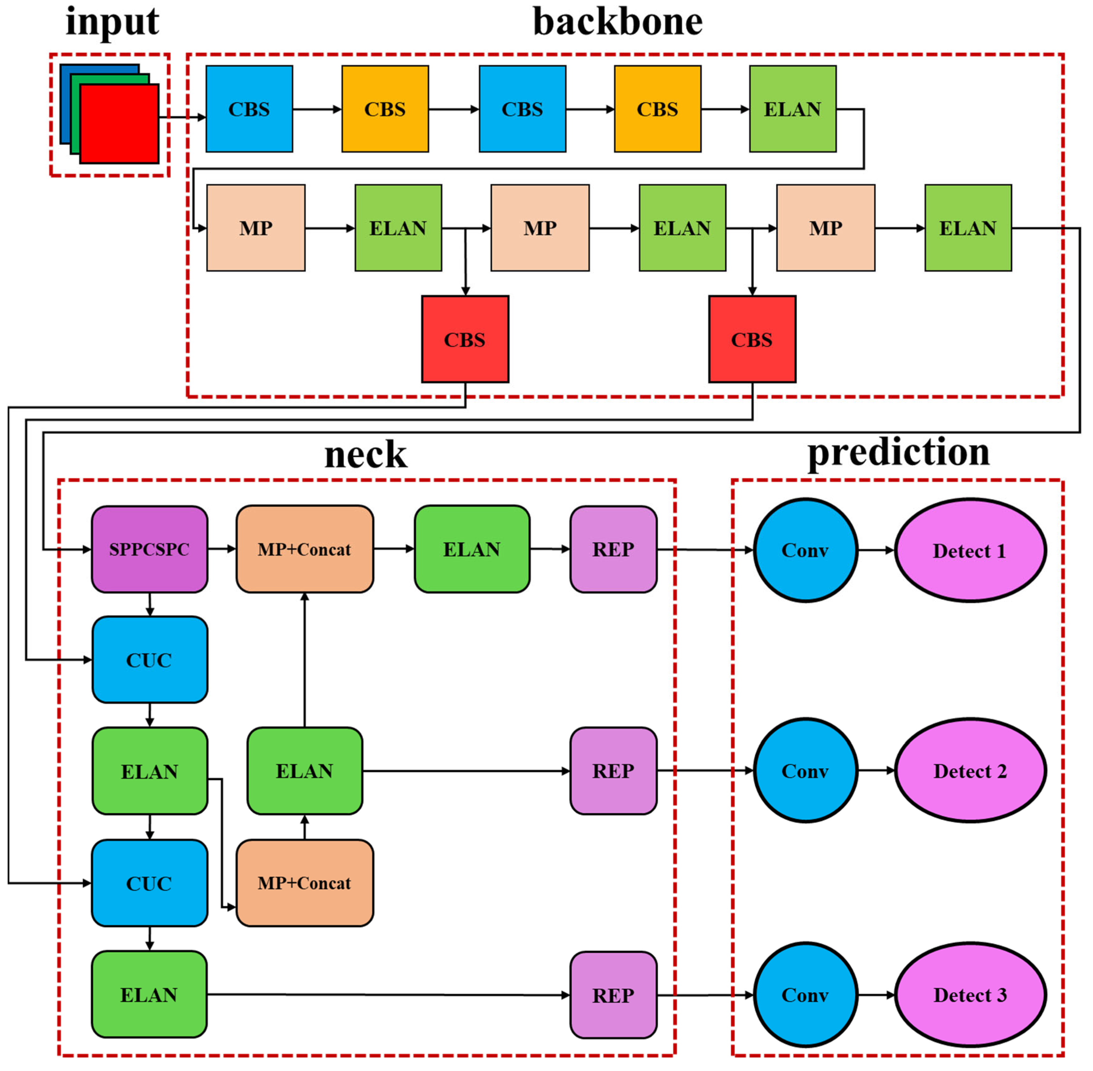
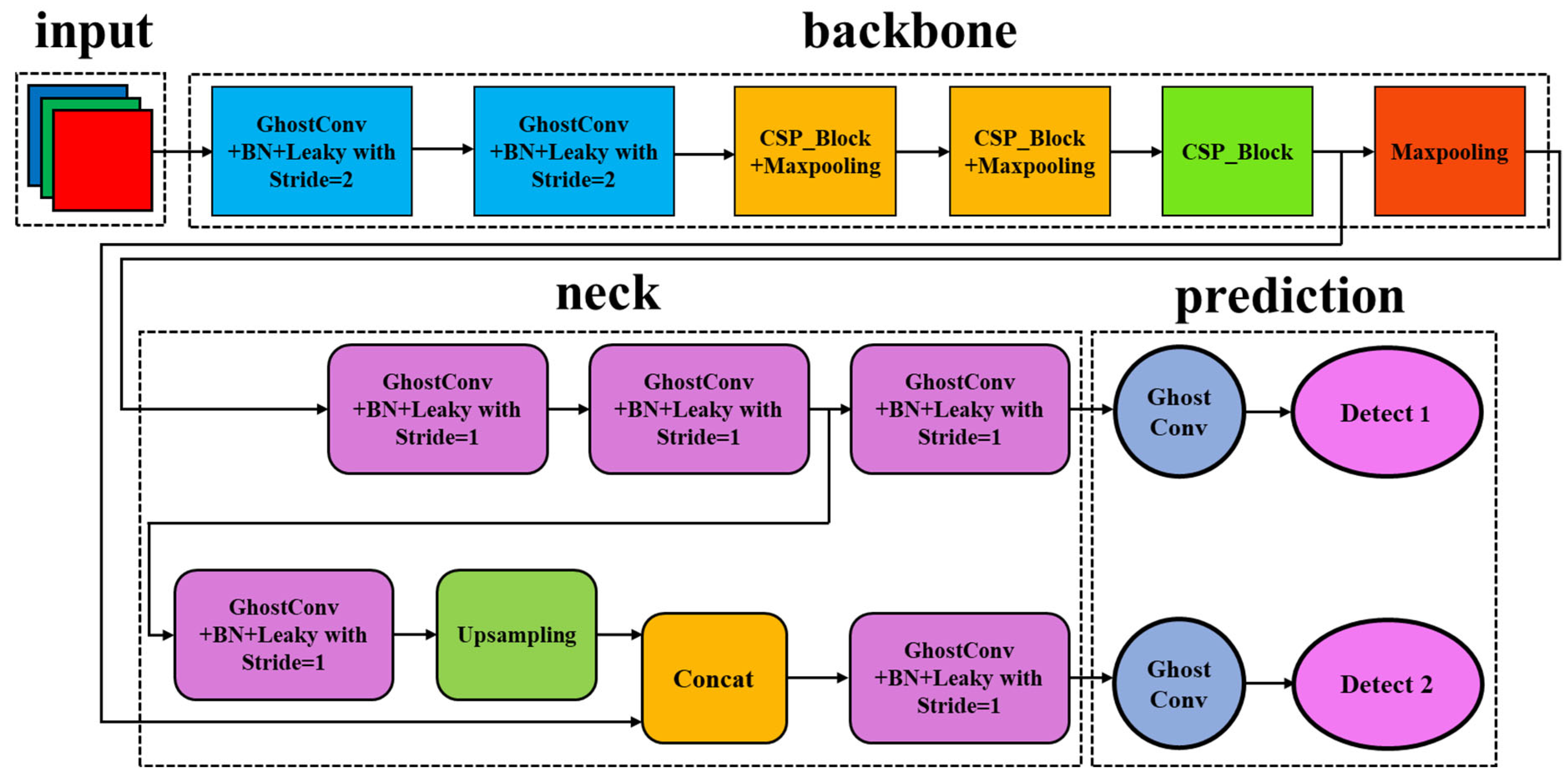
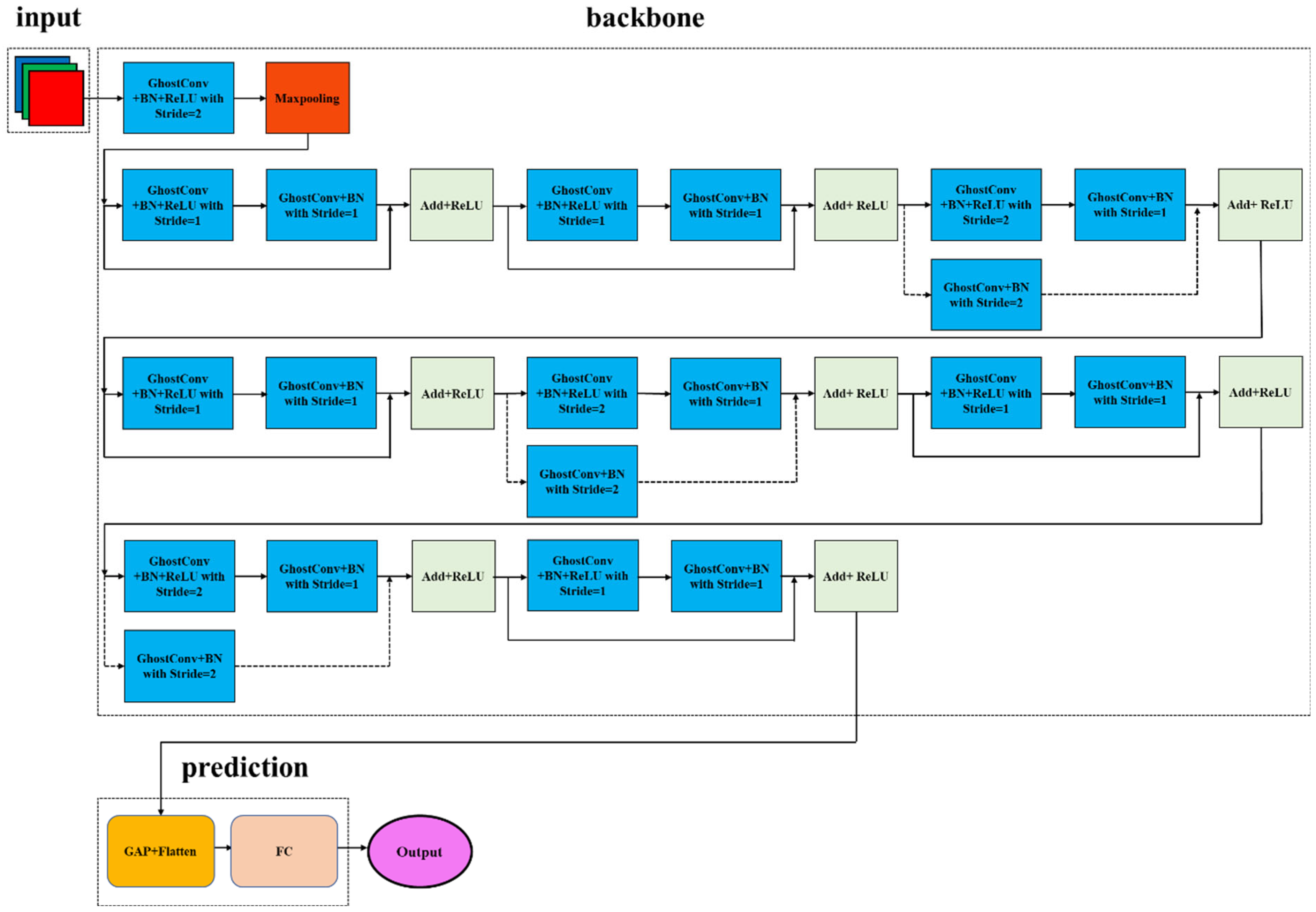
Even though YOLOv4-tiny and ResNet18 can perform precisely in object detection and steering angle prediction, we still intend to modify their network architecture to speed up the algorithm execution. If so, the new approach can shorten the response time of self-driving control to minimize the errors of driving judgment. Moreover, the model will also consume less power to realize energy-efficient object detection and steering angle prediction. Therefore, this study proposes a lightweight version of the network architecture of YOLOv4-tiny and ResNet18 to replace traditional convolution with a fast convolution within their models, where we have constructed their rapid models, abbreviated LW-YOLOv4-tiny and LW-ResNet18, as shown in Figure 10 and Figure 11, respectively. The proposed approach can significantly reduce the number of visual computations due to lightweight network architecture.

Figure 10. The architecture of the LW-YOLOv4-tiny model. (Different color means different function performed in a single block).

Figure 11. The architecture of the LW-ResNet18 model. (Different color means different function performed in a single block).

The LW-YOLOv4-tiny model comprises input, backbone, neck, and prediction, as shown in Figure 10. They replace traditional convolutions with Ghost convolutions [28] in their parts. The LW-YOLOv4-tiny model differs from the YOLOv4-tiny model, in which we use ghost convolutions instead of a traditional one and thus shorten the response time of inference intuitively. This approach will reduce the number of visual computations and enhance the ability of feature extraction to improve the inference speed without scarifying the recognition precision. The LW-ResNet18 model comprises input, backbone, and prediction, as shown in Figure 11. It has improved the inference speed like the LW-YOLOv4-tiny model to shorten the response time of the inference without sacrificing the recognition precision.

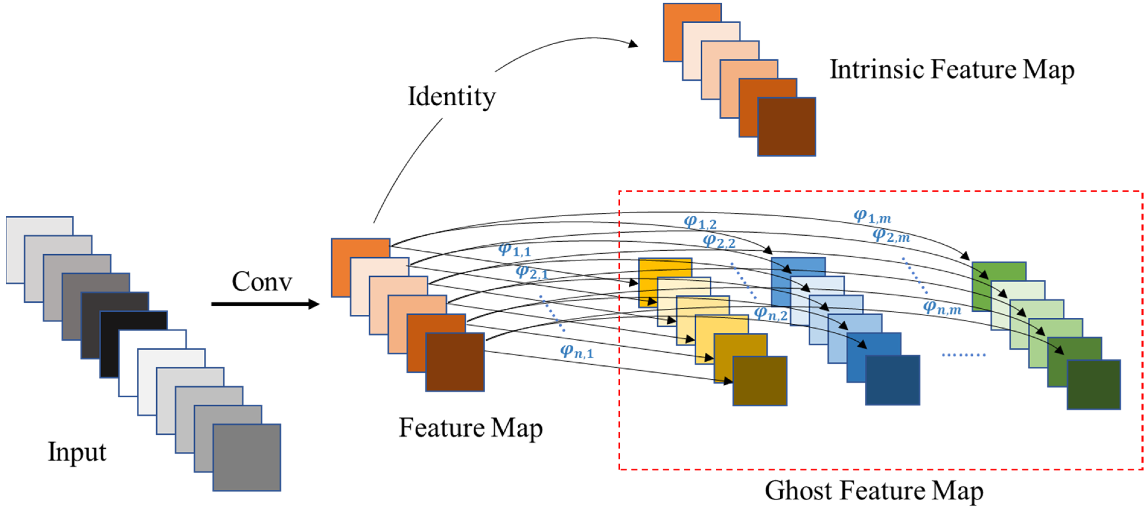
When the traditional convolutional layer performs feature extraction, the CNN-related model uses a set of filters, specifically 3 × 3 and 5 × 5 filters, to proceed with the convolution operations with the input image, and redundant information will also exist in these feature maps. Ghost convolution uses a set of ghost modules consisting of multiple network parameters (${\phi }_{i,j}, \forall i=1,2,\dots ,n, j=1,2,\dots ,m$) to perform feature extraction. This set of ghost modules executes simple linear transformation on intrinsic feature maps through network parameters ${\phi }_{i,j}$, and can generate ghost feature maps without complicated convolution operations, as shown in Figure 12. Algorithm 1 shows the ghost convolution algorithm. In Algorithm 1, intrinsic feature maps are feature maps that are calculated by traditional convolution. Then, intrinsic feature maps use ghost modules to generate more ghost feature maps through a series of simple linear transformations. The ghost feature maps can fully reveal feature information hidden in intrinsic feature maps.

Algorithm 1: Ghost Convolution

Input: Image $X$, ghost modules with linear transformation functions ${\phi }_{i,j}$

Output: $Outfm$

Obtain intrinsic feature maps $Insf{m}_i$ from a traditional convolution of image $X$ Compute the output of the ghost module: $$\begin{gathered} Ghostf{m}_{i,j}={\phi }_{i,j}\left(Insf{m}_{i,j}\right)=Wghos{t}_{i,j}\otimes Insf{m}_i\oplus Bghos{t}_{i,j} \\ \forall i=1,2,\dots ,n, j=1,2,\dots ,m \end{gathered}$$ where ${\phi }_{i,j}$ is a simplified convolution operation, $Wghos{t}_{i,j}$ shows a weight matrix of the ghost module, $Bghos{t}_{i,j}$ implies a bias matrix of the ghost module, $n$ represents the number of intrinsic feature maps, $m$ stands for the number of the ghost modules, the symbol $\otimes$ denotes the pixel-wise product of two matrixes, and the symbol $\oplus$ indicates the pixel-wise sum of two matrixes. Transform intrinsic feature maps $Insf{m}_i$ into the ghost feature maps $Ghostf{m}_{i,j}$, with multiple ghost modules. $\begin{array}{cc}Outfm\hfill & =\left\{Outf{m}_1,Outf{m}_2,\dots , Outf{m}_n\right\}=\left\{Outf{m}_i, \forall i=1,2,\dots ,n \right\}\hfill \\ Outf{m}_i\hfill & =\left\{Insf{m}_i, Ghostf{m}_{i.1}, Ghostf{m}_{i.2},\dots ,Ghostf{m}_{i.m}\right\}\hfill \\ & =\left\{Insf{m}_i, Ghostf{m}_{i.j}, \forall j=1,2,\dots ,m \right\}\hfill \end{array}$ where $Outf{m}_i$ represents the output feature maps, including the corresponding intrinsic feature map and ghost feature maps, and $Outfm$ stands for the whole output feature maps in a convolution layer.

Figure 12. Execution flow of ghost convolution.

Generally, the CNN-related model uses many filters in traditional convolution operations, and the number of filters must be consistent with the number of output channels. Technically speaking, in Figure 12, ghost convolution can obtain intrinsic feature maps after performing traditional convolution operations on a set of filters and then generate more ghost feature maps through simple linear transformation directly. This approach can significantly avoid a substantial amount of time-consuming traditional convolution operations. Assume that $r$ represents the side length of the output feature map, $s$ stands for the side length of the filter, $c$ indicates the number of channels of the input feature map, $h$ denotes the number of channels of the output feature map, and $v$ implies the number of channels of a set of filters of the output feature map through a traditional convolution operation, $l$ shows an index of the convolutional layer, and $u$ is the number of convolutional layers. According to the discussion in [29], the time complexity of the traditional convolutional layer is O(${\displaystyle {\displaystyle \sum }_{l=1}^u}{r}_l^2·s_l^2·c_l·h_l$), while the time complexity of ghost convolution is O(${\displaystyle {\displaystyle \sum }_{l=1}^u}(r_l^2·s_l^2·c_l·v_l+r_l^2·\left(h_l-v_l\right))$), which is much less than the former one. Therefore, compared with the traditional convolution layer, the time complexity of ghost convolution is much smaller, so it can significantly reduce the cost of convolution calculation. This approach has given new (ghost) feature maps without redundant information, thus slightly improving the prediction accuracy.

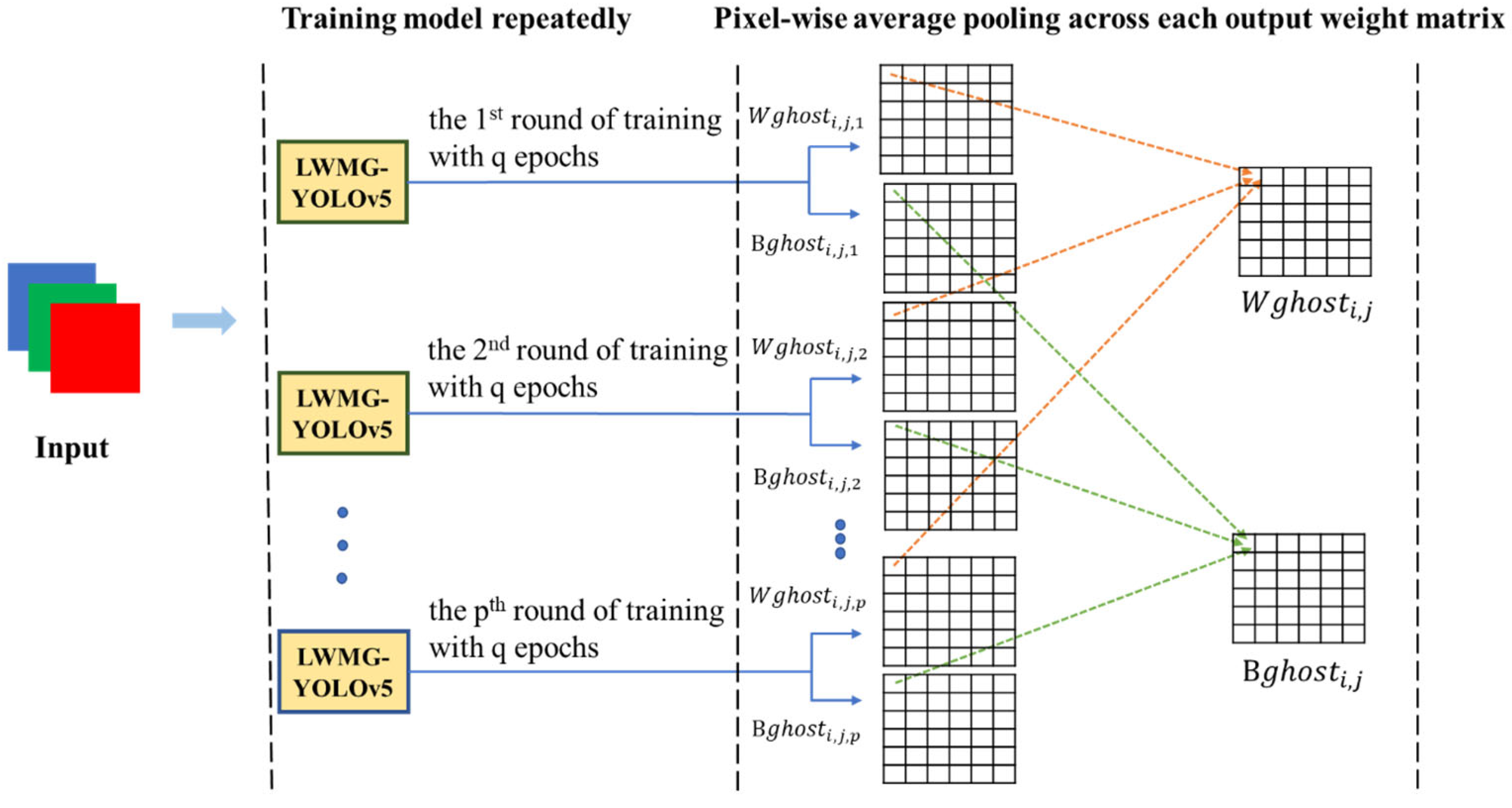
In the training phase, the CNN-related model uses the steepest gradient descent algorithm to continuously update the weight matrix $Wghos{t}_{i,j}$ and the bias matrix $Bghos{t}_{i,j}$, achieving the best results of matrixes. The weight matrix $Wghos{t}_{i,j}$ and the bias matrix $Bghos{t}_{i,j}$, which are obtained from a single round of network training, are not necessarily reliable, so this study proposes pixel-wise average pooling to obtain a more reliable $Wghos{t}_{i,j}$ and $Bghos{t}_{i,j}$, as shown in Figure 13. Assuming that there are $p$ rounds of training, each training carries out for $\mathrm{q}$ epochs. When the training runs out of all epochs for each round, it can obtain the final weight matrix $Wghos{t}_{i,j,k}$ ($\forall i=1,2,\dots ,n, j=1,2,\dots ,m, k=1,2,\dots ,p$), and the final bias matrix $Bghos{t}_{i,j,k}$ ($\forall i=1,2,\dots ,n, j=1,2,\dots ,m, k=1,2,\dots ,p$). After $p$ rounds of network training, the training process will perform pixel-wise average pooling on the weight matrixes and bias matrixes, and the average value of the corresponding element positions in $p$ weight matrices and $p$ bias matrices can obtain a more reliable $Wghos{t}_{i,j}$ and $Bghos{t}_{i,j}$. The linear transformation that such ghost convolution uses can extract features with more precision and obtain higher prediction accuracy for subsequent inferences.

Figure 13. Pixel-wise average pooling.

3.4. Distance Measurement and PID Control

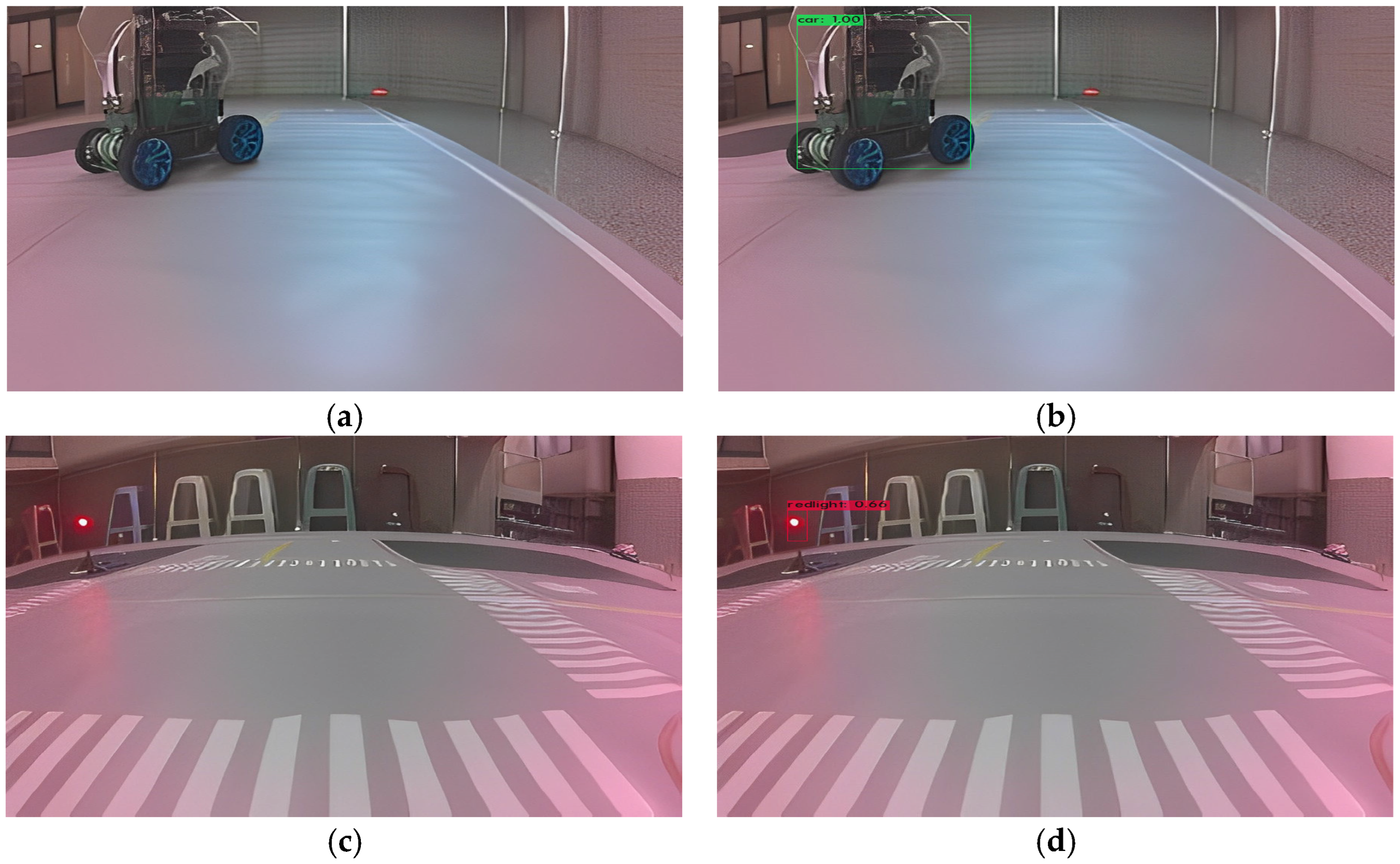
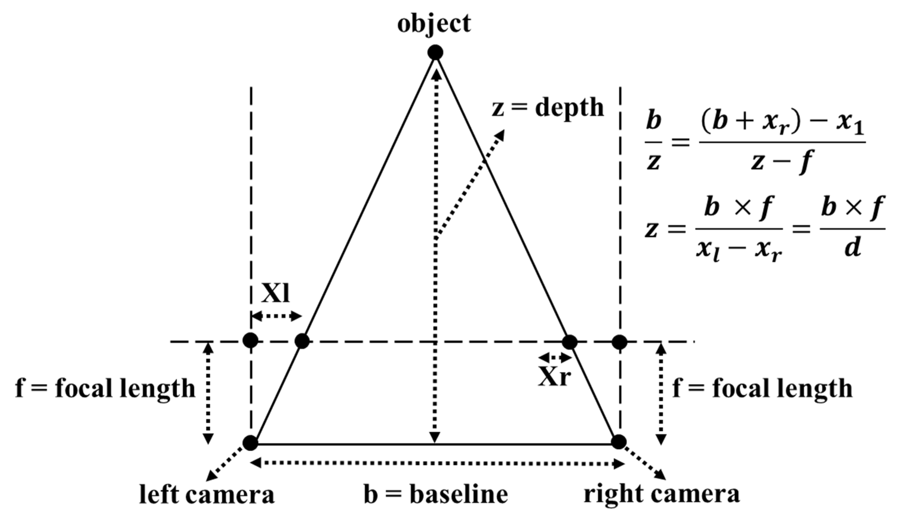
In Figure 14 and Figure 15, LW-YOLOv4-tiny proceeds with object detection in the real-time video streaming captured from the dual cameras located in the front and rear panels of JetRacer. This study uses visual odometry to measure the distance between the vehicle and the target object, as shown in Figure 16. The triangle theorem and the principle of parallax can estimate the distance between the detected object and the center point at the horizontal line spanned dual cameras, as shown in Figure 17. However, there are some restrictions on the use of dual cameras, including the fixed distance between the dual cameras and the build of the dual cameras on the same horizontal line. Otherwise, they will significantly affect the accuracy of measuring distance.

Figure 14. Real-time object detection by using LW-YOLOv4-tiny. (a) Real-time image of model car one on the outer lane. (b) Real-time object detection of model car one on the outer lane. (c) Real-time image of model car two on the inner lane. (d) Real-time object detection of model car two on the inner lane.

Figure 15. Real-time vehicle detection by using LW-YOLOv4-tiny. (a) Left camera module. (b) Right camera module.

Figure 16. Measuring distance between the vehicle and the target object.

Figure 17. Measuring the distance between two JetRacers by using dual cameras. (a) Left camera. (b) Right camera.

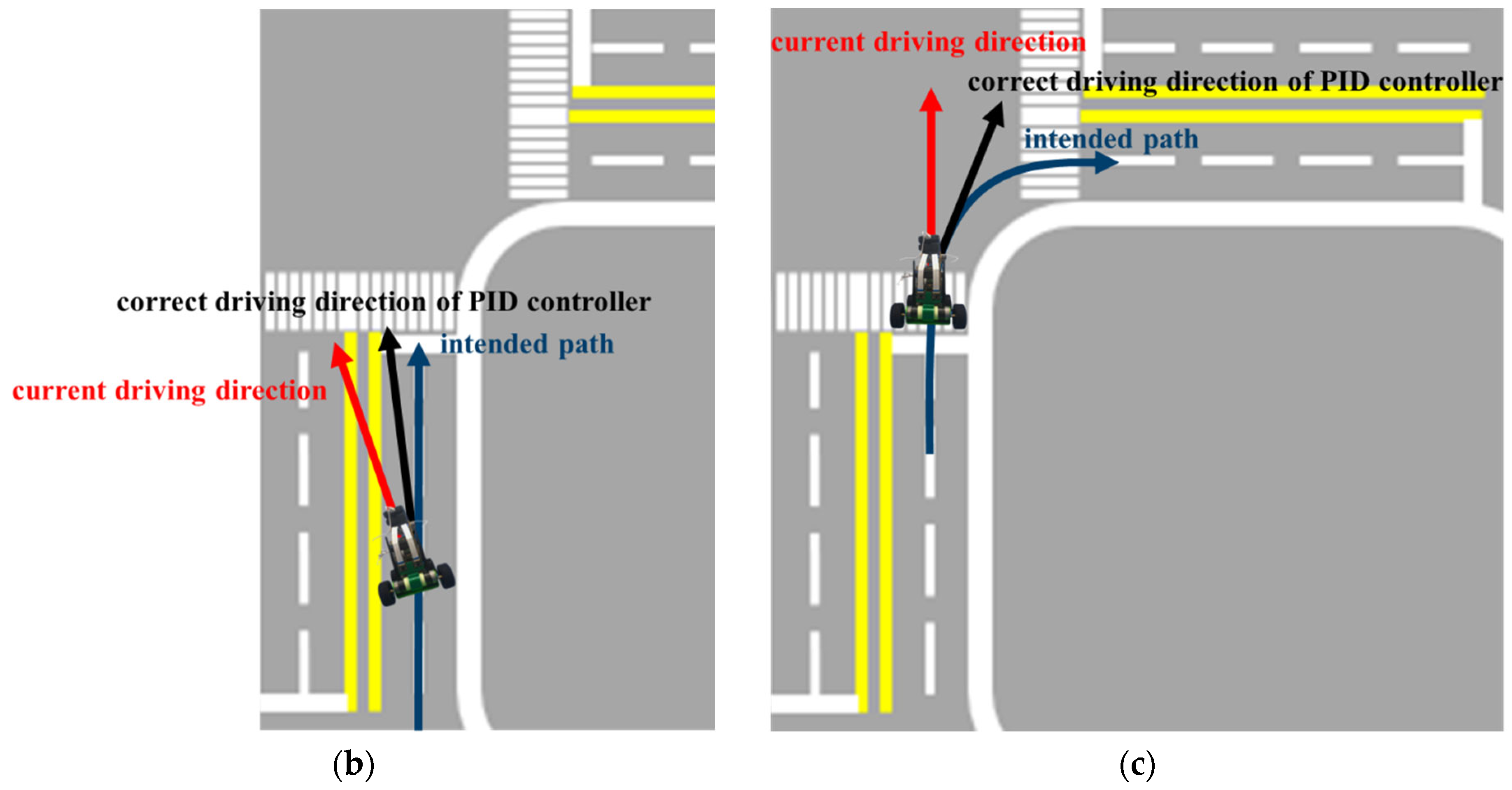
In Figure 18, LW-ResNet18 predicts the steering angle along the route while JetRacer moves forward. The keen steering angle changes, resulting partially from the fact that the predicted value may cause the model car to shake from side to side while moving, causing JetRacer to swing significantly along the route. Therefore, as shown in Figure 19, we add the PID controller to the autonomous driving system, which includes proportional control with the parameter $K_p$, integral control with the parameter $K_i$, and differential control with the parameter $K_d$. The purpose of proportional control is that the more JetRacer deviates from the lane, the greater the degree of correction back to the original lane. Integral control aims to sum up all error values and conduct reverse correction for the direction with much more deviation. Differential control aims to correct the offset in the opposite direction to avoid the excessive correction caused by only the parameter $K_p$. Table 1 gives the default settings of three PID parameters.

Figure 18. Steering angle prediction by using LW-ResNet18.

Figure 19. PID controller. (a) The architecture of the PID controller; (b) going straight; (c) taking a right turn.

Table 1. Parameter setting of PID controller.

Parameter	$K_p$	$K_i$	$K_d$
Value	0.06	0.0015	1.52

3.5. Information Fusion and Visualized Steering Assistance

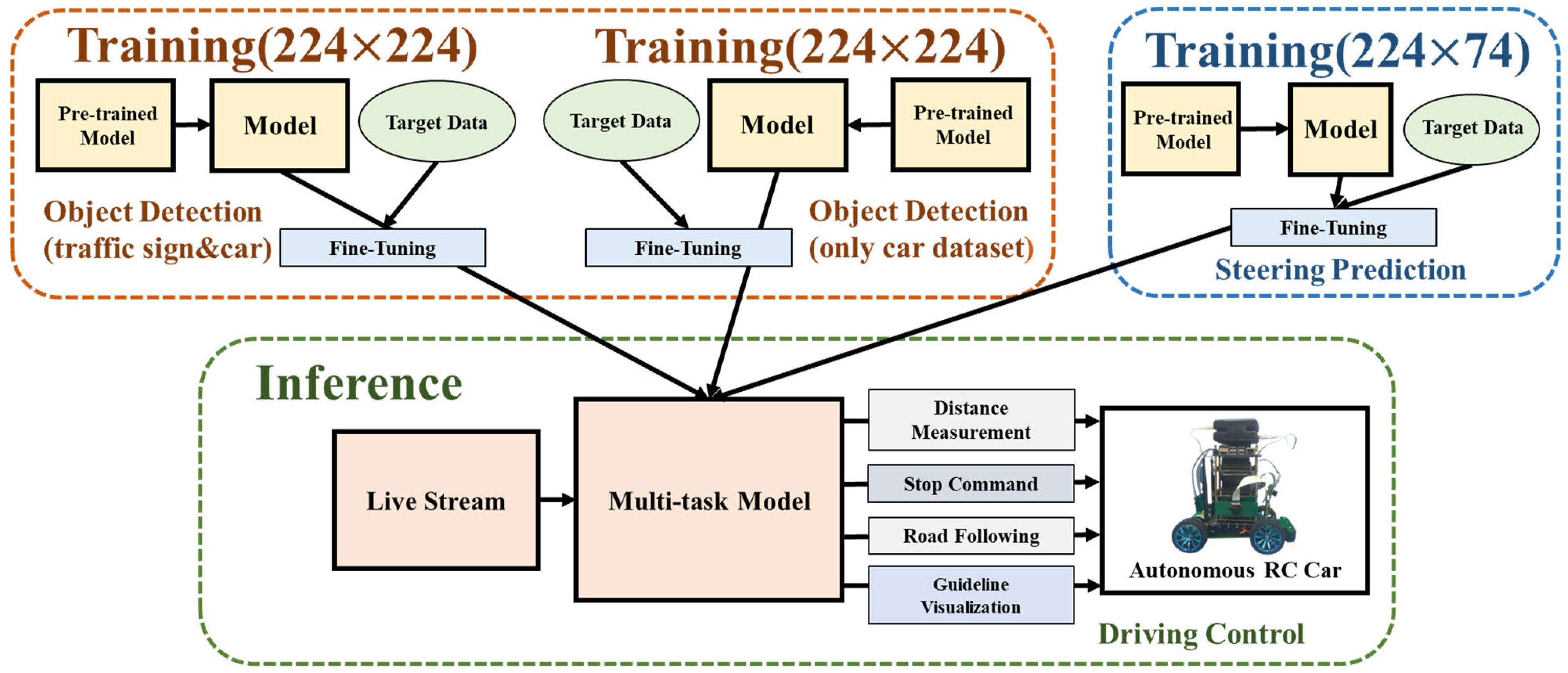
This study uses the integration of YOLOv4-tiny and ResNet18 models to achieve autonomous driving functions, which have successfully implemented object detection and image recognition in the embedded platforms Jetson Nano on a JetRacer. Image recognition allows JetRacer to learn how to drive on the routes correctly in a planar road map. Object detection identifies the traffic signs and other vehicles on the road, especially in real-time, measuring the approximate distance between the vehicle and the target object through dual cameras to avoid a collision. Figure 20 shows the system diagram of the autonomous driving system proposed in this study.

Figure 20. System diagram of the autonomous driving system.

Typically, steering angle prediction and object detection will run continuously across the planar road map. An autonomous driving system needs a mechanism that requires information fusion between the two processes during the driving of the model car. First, when the object detection has recognized a red light or a stop sign in front of the model car, the Jetracer will brake accordingly. If the steering angle prediction has decided to turn left or right at that time and the driving system does not ignore this action, it will cause the Jetracer to be stationary, but its front wheels will move left and right, as mentioned above. Next, when the object detection recognizes the speed limit sign, the system should adjust the driving speed of the Jetracer according to the speed limit. Then, there is the decision to turn left or right. Jetracer has to maintain a constant speed to avoid the doubt of insufficient corner entry. Finally, there is the decision to go straight. The steering value should be fixed at 0 so that the Jetracer can stably go straight on the straight road. Therefore, the autonomous driving system takes information fusion to deal with the contradiction problems caused by inconsistent driving decision-making. Figure 21 shows the decision-making performed by Jetracer in various scenarios to avoid unreasonable driving behavior.

Figure 21. Information fusion of self-driving.

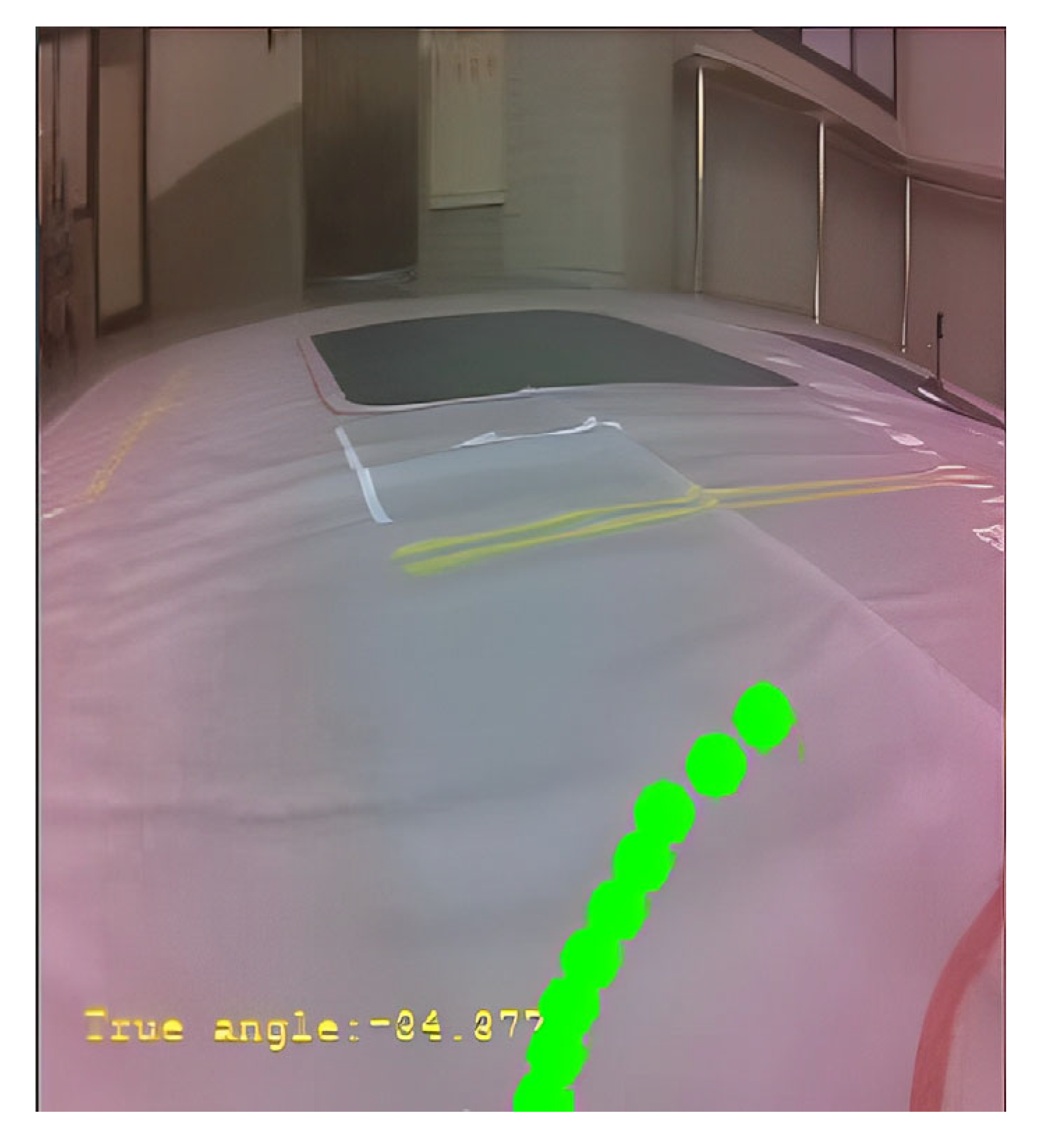
According to the steering range on the real-time image in the form of a JetRacer, the autonomous driving system creates a green dot line that presents visualized steering assistance for guiding the imminent turning direction of a JetRacer, as shown in Figure 22. The purpose of visualized steering assistance is to remind the driver of a forecast of the imminent turning direction of a JetRacer. When the autonomous driving system deviates, and the JetRacer is about to deviate from the lane, manual driving by the driver can cause the JetRacer to return to the original lane, which ensures a safe drive.

Figure 22. A green dot line as a visualized steering assistance.

4. Experiment Results and Discussion

This study tested the object detection algorithms as follows: LW-YOLOv4-tiny, YOLOv4-tiny [1], YOLOv5s [24], YOLOv5n [30], YOLOv7 [26], and YOLOv7-tiny [26]. Regarding the steering angle prediction algorithms, this study tested Nvidia-CNN [8], traditional convolutional neural networks (CNN) [31], ResNet18 [3], and LW-ResNet18. The Nvidia-CNN mentioned in [8] refers to a specific convolutional neural network architecture developed by NVIDIA Corporation for image recognition and steering angle prediction tasks for self-driving cars. Compared with CNN, the architecture of NVIDIA-CNN is relatively simple, including only convolutional layers and fully connected layers, and uses a smaller filter, which is suitable for processing tasks such as image classification. The experiments have trained five object detection models and three steering angle prediction models in different combinations executed in Jetson Nano and implemented in JetRacer for autonomous driving.

4.1. Experiment Setting

The hardware specifications used in the experiments are GPU workstation and embedded platform Jetson Nano, as listed in Table 2. Table 3 lists the recipe of packages used in the experiments.

Table 2. Hardware specifications.

Component	GPU Workstation	Jetson Nano
GPU	NVIDIA GeForce GTX 1080 Ti	NVIDIA Maxwell architecture with 128 NVIDIA CUDA® cores
CPU	Intel (R) Core (TM) i7-7700 CPU @ 3.60 GHz	Quad-core ARM Cortex-A57 MPCore processor
Memory	32 GB	4 GB 64-bit LPDDR4, 1600 MHz 25.6 GB/s
Storage	256 GB × 1 (SSD) 1 TB × 1 (HDD)	16 GB eMMC 5.1

Table 3. Recipe of packages.

Software	Version
LabelImg	1.8
Anaconda® Individual Edition	4.9.2
Jupyter Notebook	6.1.4
TensorFlow	2.2
TensorRT	7.2.3
PyTorch	1.6
JetPack	4.5

4.2. Model Training, Inference, and Capability

The input image source is a set of 1476 images as a training dataset and 366 as a test dataset. We have collected approximately the same amount for each class to be identified, based on approximately 65% training set, 16% validation set, and 16% test set. They are relatively close to the commonly used distribution with the ratio of 60% training set, 20% validation set, and 20% test set. Several object detection models are operated in the GPU workstation, as listed in Table 4. For the same group of training data, the experiment recorded the time spent on training in the GPU workstation, and Equation (1) calculates the total inference time required for every model to detect the objects from test images where $I{T}_i$ denotes inference time (IT), $i$ represents the inference using the $i$th object detection model, $I$ stands for the total number of object detection models, $x$ is the $x$th test image, $X$ shows the total number of test images, and $EI{T}_i$ indicates the time taken to complete the inference for each test image.

$$I{T}_i={\displaystyle \sum }_{x=1}^{X}EI{T}_i, where i=1, 2, \dots , I, x=1, 2,\dots , X$$

(1)

Table 4. Training and inference time of object detection models (unit: s).

Method	LW-YOLOv4-Tiny	YOLOv4-Tiny	YOLOv5s	YOLOv5n	YOLOv7	YOLOv7-Tiny
Training	274	296	497	436	2124	1314
Inference	4.98	5.32	6.64	6.48	10.68	5.75

The test image size is 224 × 224, and the number of iterations is 50. In Table 4, the first row shows the time to train every object detection model with the same parameter settings. The second one calculates the time to implement inference from 366 test images. The experimental results showed the training and inference time of every object detection model, and LW-YOLOv4-tiny bests the others.

The input image source is a training dataset of 14,710 images, and there are three different steering angle prediction models that are operated in a GPU workstation, as listed in Table 5. For the same group of training data, the experiment recorded the training time in a GPU workstation, and Equation (1) calculates the total inference time required for every steering angle prediction model to predict the steering angle of 1000 test images, where $i$ represents using the $i$th steering angle prediction model for image inference.

Table 5. Training and inference time of steering angle prediction models (unit: s).

Method	LW-ResNet18	ResNet18	CNN	Nvidia-CNN
Training	2832	2880	360	364
Inference	23.79	25.18	21.27	21.56

The test image size is 224 × 74, and the number of iterations is 30. In Table 5, the first row shows the time to train every steering angle prediction model with the same parameter settings. The second one calculates the time to implement inference from 1000 test images. Although the training time of the steering angle prediction model ResNet18 is much longer than that of the others, its inference time is slightly better than that of the others.

Table 6 lists the number of parameters every object detection model uses. In Table 6, the YOLOv7 model has the most significant number of parameters, and the YOLOv5n model has the least. In contrast, Table 7 lists the parameters used by every steering angle prediction model. In Table 7, the ResNet18 model has the most significant number of parameters, and the CNN model has the least.

Table 6. Parameters of object detection models.

Method	LW-YOLOv4-Tiny	YOLOv4-Tiny	YOLOv5s	YOLOv5n	YOLOv7	YOLOv7-Tiny
Number of parameters	3,940,751	5,892,596	7,043,902	1,776,094	37,239,708	6,036,636

Table 7. Parameters of steering angle prediction models.

Method	LW-ResNet18	ResNet18	CNN	Nvidia-CNN
Number of parameters	6,367,975	11,180,161	776,289	1,872,643

4.3. Training and Validation Losses

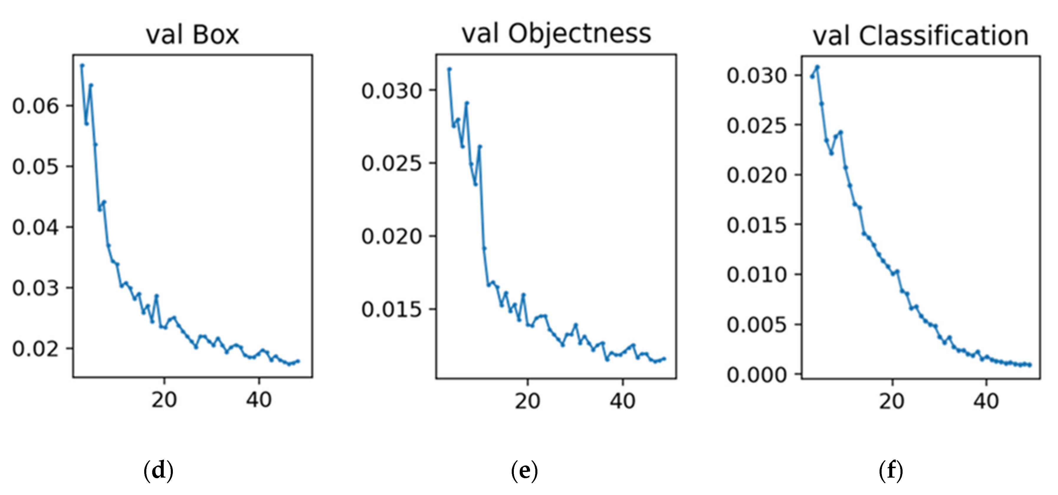
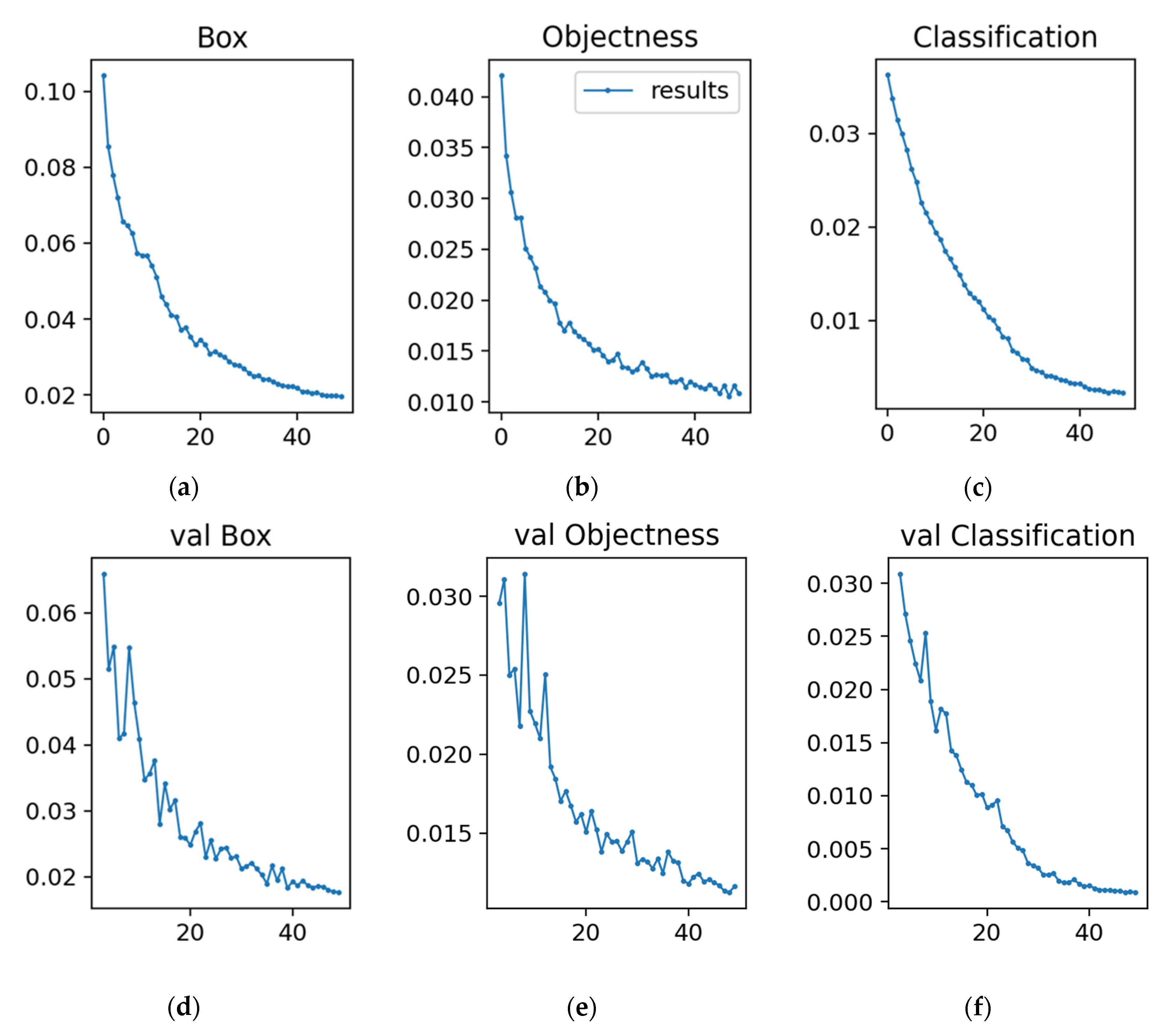
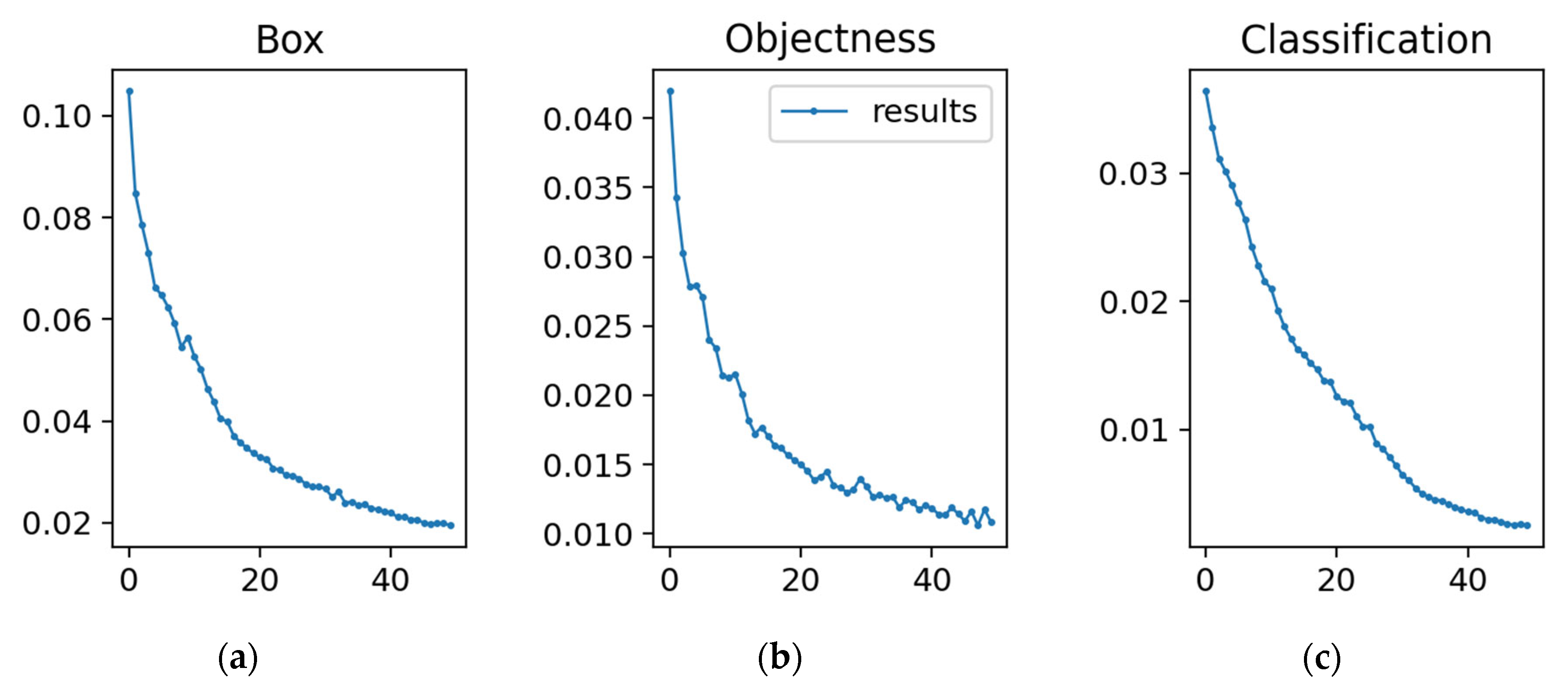
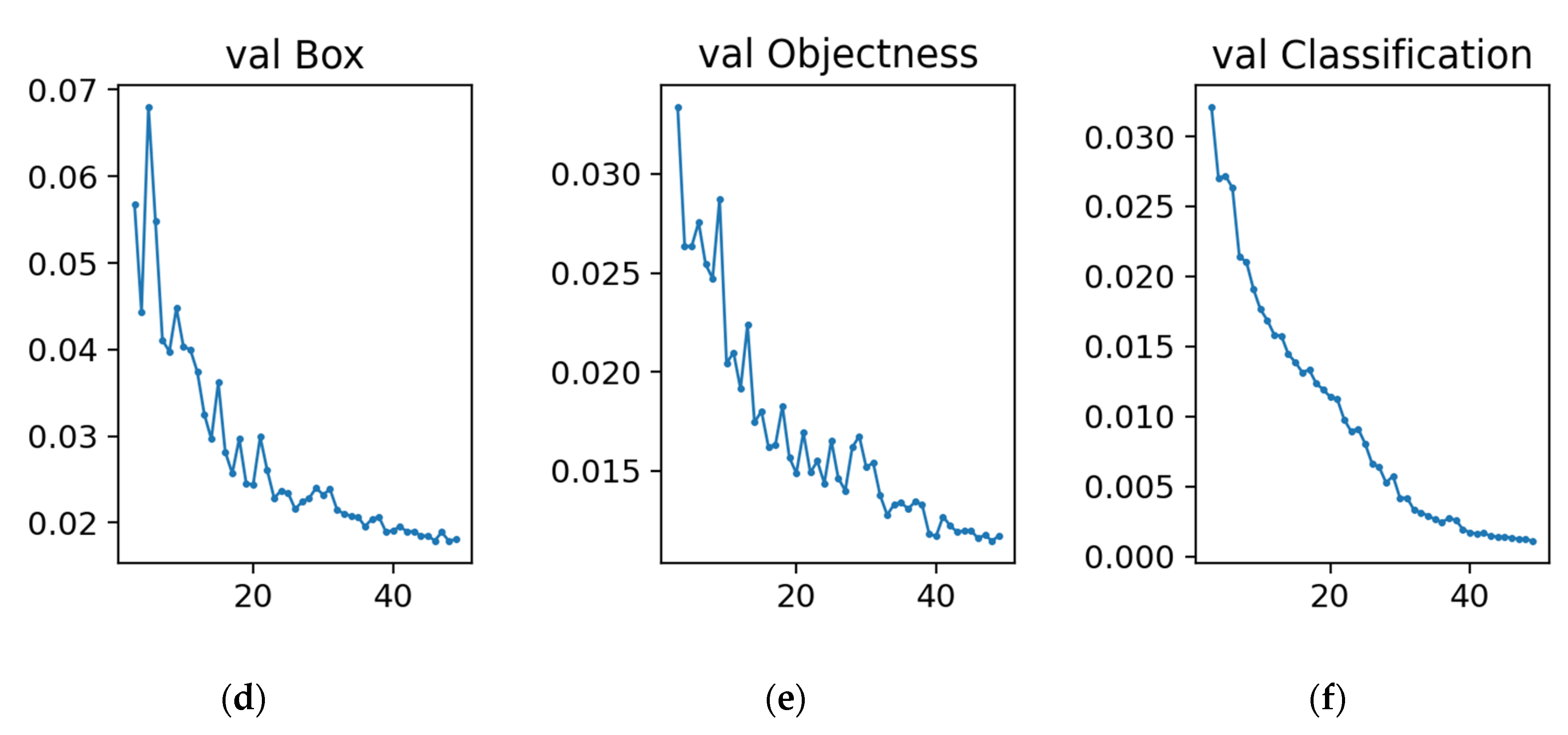
After 50 training epochs, we used the visualization tool to observe the training process and the callback function to save the best-performance model. Every object detection model has six loss plots, as shown in Figure 23, Figure 24, Figure 25, Figure 26, Figure 27 and Figure 28. In Figure 23, Figure 24, Figure 25, Figure 26, Figure 27 and Figure 28, the upper row shows the training losses, and the lower row shows the verification losses, where the first column is the positioning loss and the second is the confidence level loss. The third is the loss of whether the predicted frame matches the actual frame. The verification has shown that every object detection model can stably drop to the minimum loss.

Figure 23. Training and validation losses of the LW-YOLOv4-tiny model. (a) Box training loss. (b) Objectness training loss. (c) Classification training loss. (d) Box validation loss. (e) Objectness validation loss. (f) Classification validation loss.

Figure 24. Training and validation losses of the YOLOv4-tiny model. (a) Box training loss. (b) Objectness training loss. (c) Classification training loss. (d) Box validation loss. (e) Objectness validation loss. (f) Classification validation loss.

Figure 25. Training and validation losses of the YOLOv5s model. (a) Box training loss. (b) Objectness training loss. (c) Classification training loss. (d) Box validation loss. (e) Objectness validation loss. (f) Classification validation loss.

Figure 26. Training and validation losses of the YOLOv5n model. (a) Box training loss. (b) Objectness training loss. (c) Classification training loss. (d) Box validation loss. (e) Objectness validation loss. (f) Classification validation loss.

Figure 27. Training and validation losses of the YOLOv7 model. (a) Box training loss. (b) Objectness training loss. (c) Classification training loss. (d) Box validation loss. (e) Objectness validation loss. (f) Classification validation loss.

Figure 28. Training and validation losses of the YOLOv7-tiny model. (a) Box training loss. (b) Objectness training loss. (c) Classification training loss. (d) Box validation loss. (e) Objectness validation loss. (f) Classification validation loss.

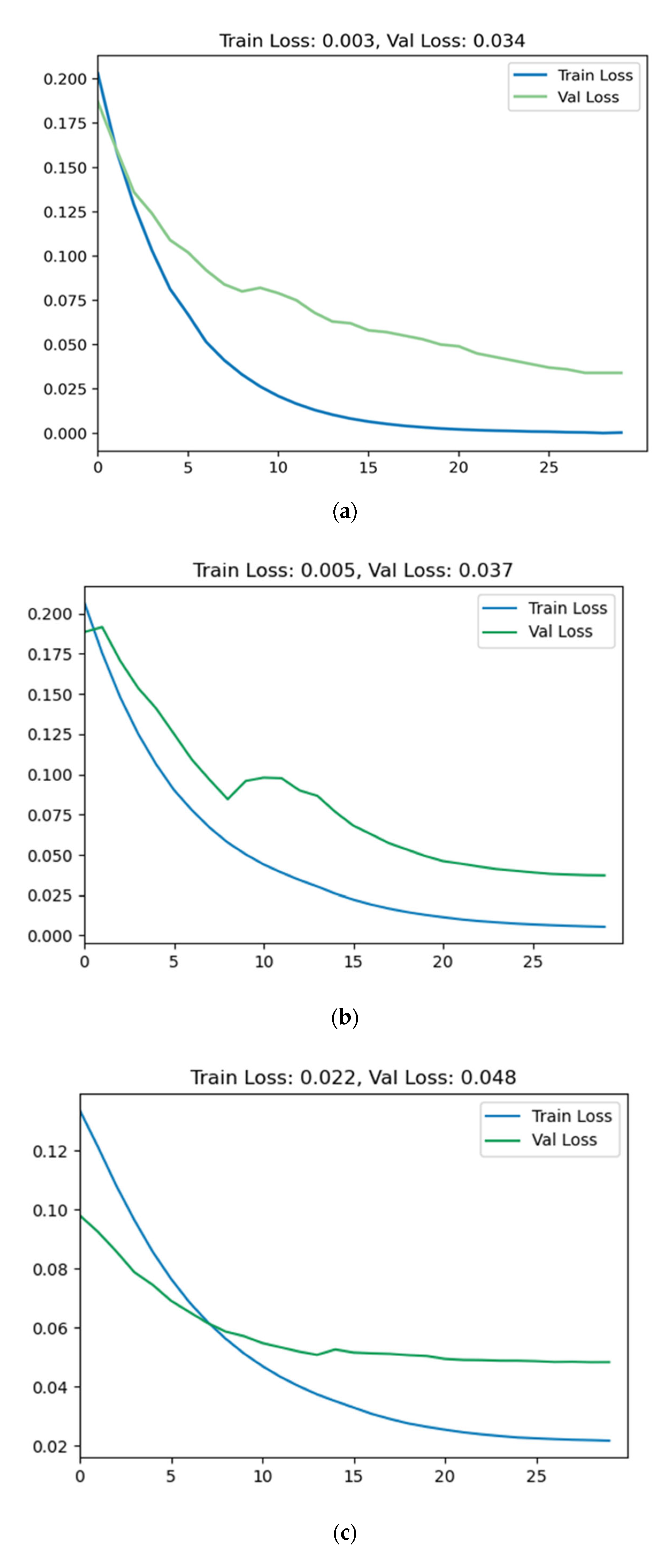
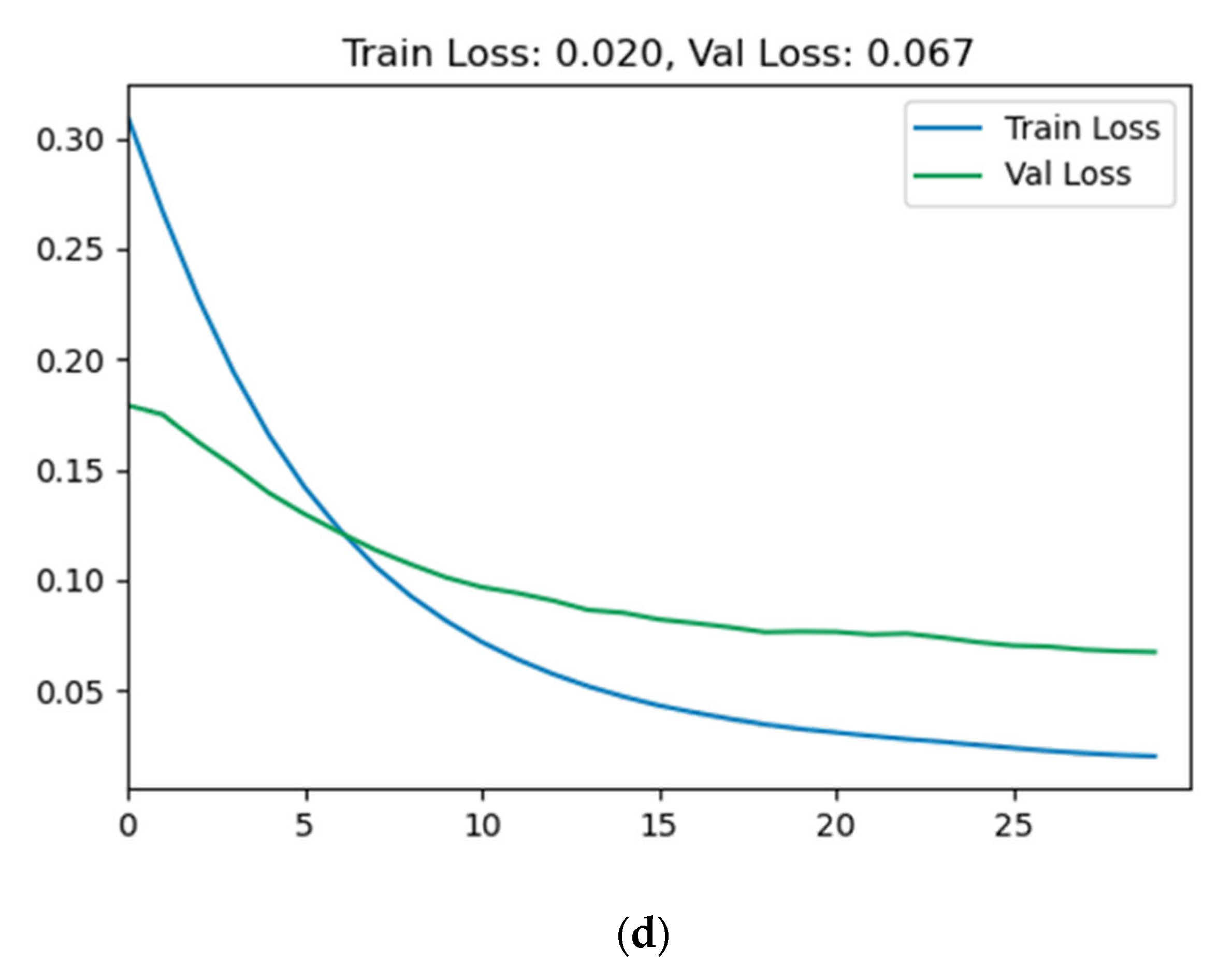
After 30 training epochs, we used the visualization tool to observe the training process and the callback function to save the best-performance model. There are three loss plots for every steering angle prediction model, as shown in Figure 29. In Figure 29, the blue line represents the training loss, and the green line represents the verification loss. LW-ResNet18 model can reduce the verification loss to 0.034, ResNet18 model 0.037, CNN model 0.048, and Nvidia-CNN model 0.067.

Figure 29. Training and validation losses of steering angle prediction model. (a) LW-ResNet18. (b) ResNet18. (c) CNN. (d) Nvidia-CNN.

4.4. Model Testing

Equation (2) can evaluate the execution speed of object detection denoted frames per second (FPS), where the $FP{S}_j$ is the FPS of the $j$th object detection model, $J$ represents the number of all object detection models, and $IRAI{T}_j$ stands for the time required for each image in real-time object detection by using the $j$th object detection model.

$$FP{S}_j=\frac{1}{IRAI{T}_j}, where j=1, 2,\dots , J$$

(2)

The mean Average Precision (mAP) of all categories can evaluate the precision of object detection, which calculates the mean of all the average precisions of each category. Equation (3) calculates the precision $mA{P}_l$ of all object detection models, where $L$ represents the number of all object detection models, $mA{P}_l$ stands for the mean Average Precision of the $l$th object detection model, $C_l$ is the number of identified categories in the $l$th model, $k_l$ denotes a specific category in the $l$th model, and $A{P}_{k_l}$ indicates the precision of a specific category in the $l$th model.

$$mA{P}_l=\frac{{{\displaystyle \sum }}_{k_l=1}^{C_l}A{P}_{k_l}}{C_l}, where k_l=1, 2, \dots , C_l, l=1,2,\dots ,L$$

(3)

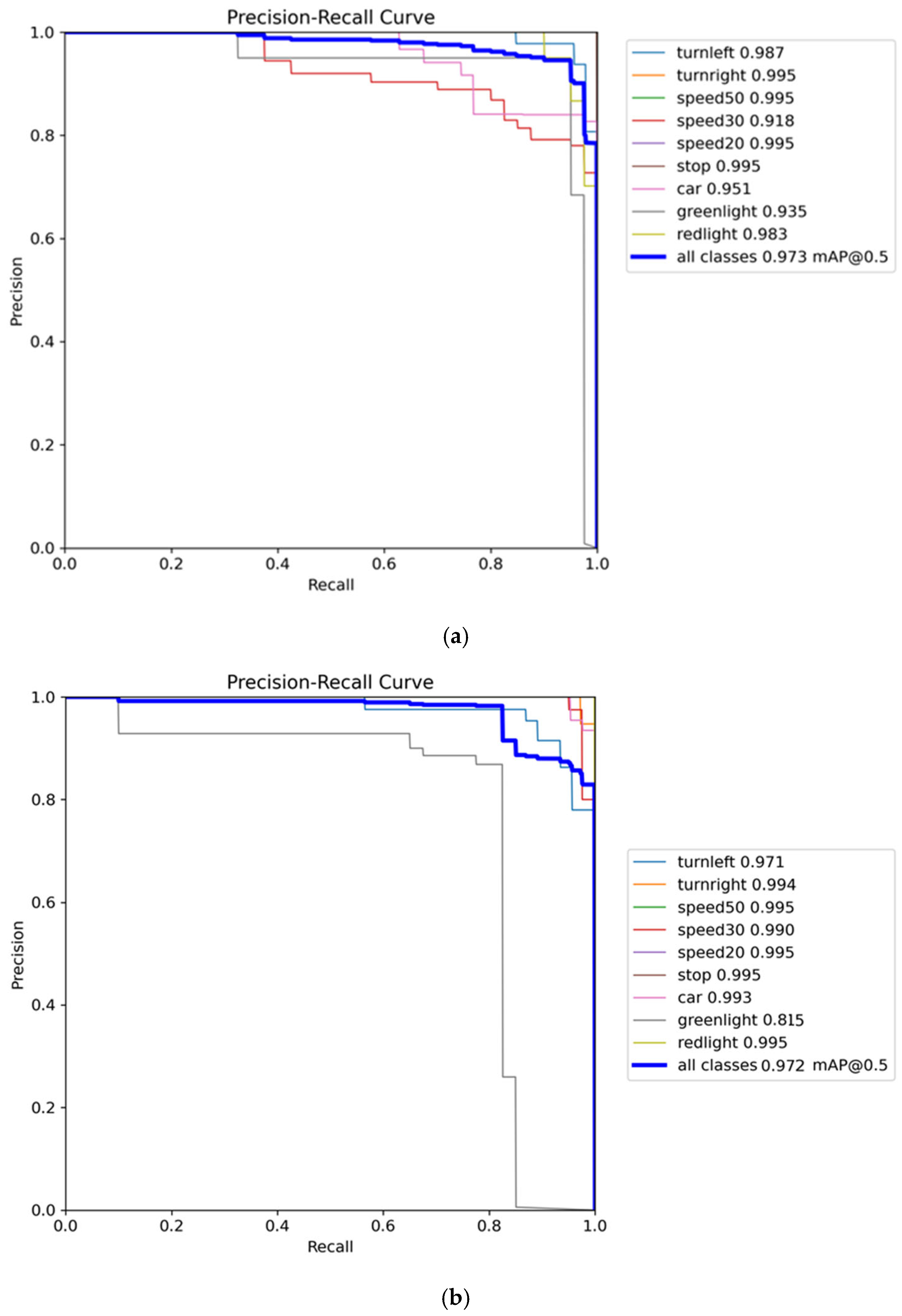
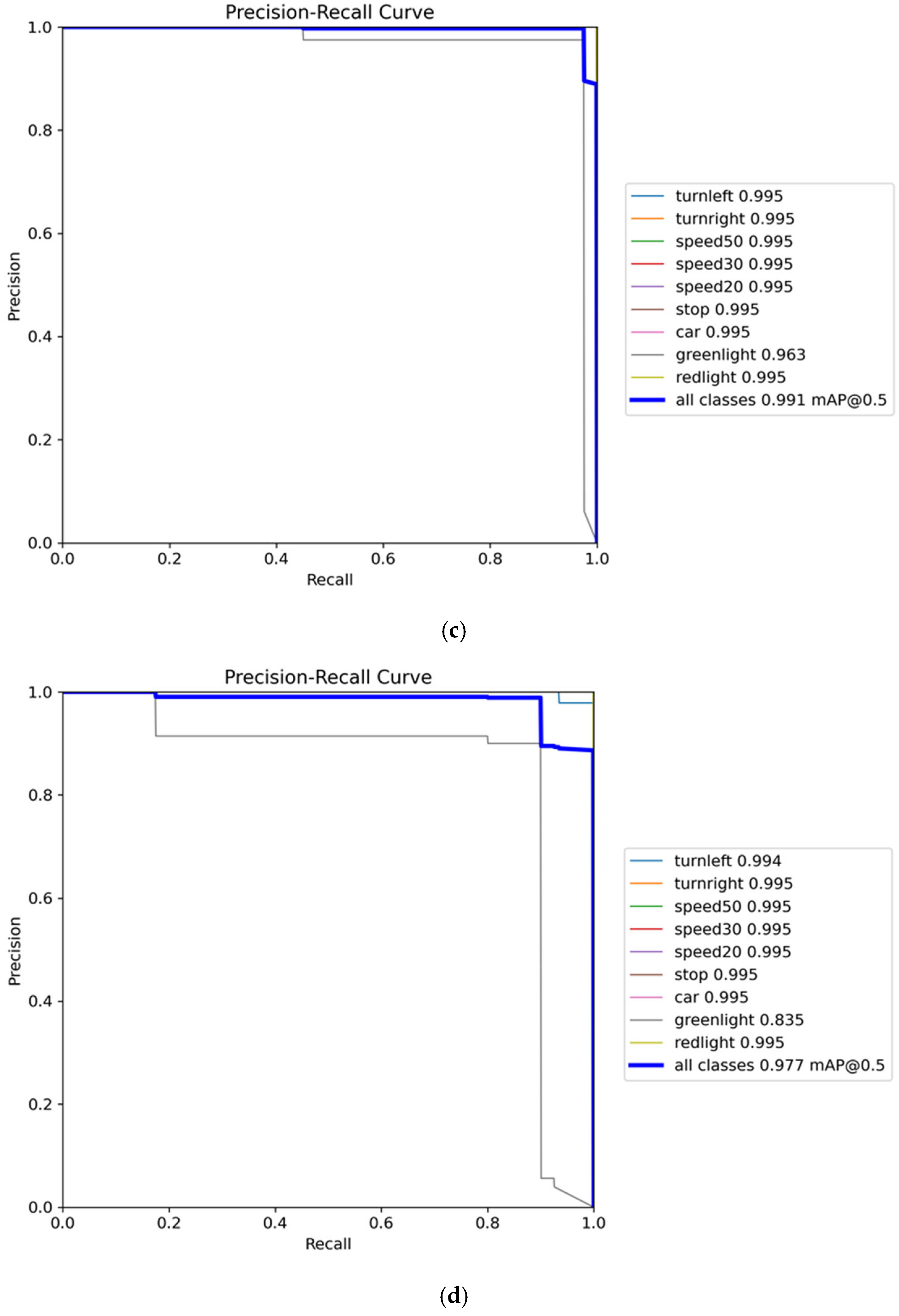
Here, we will evaluate the execution speed and precision of every object detection model. After the models were trained with the same parameter settings, the experiment tested the trained models with 366 images and plotted the PR curve results, as shown in Figure 30. In the test, Equation (2) computes the execution speed FPS, and Equation (3) evaluates the precision mAP, as listed in Table 8. In Figure 30, the PR curve takes recall as the x-axis and precision as the y-axis, and each point represents a combination of recall and precision. Next, we can obtain an AP by averaging all precisions retrieved from the combinations. The mAP is the sum of the APs from all categories in the PR curves and then divided by the total number of categories. In Table 8, YOLOv5s achieve the best precision, and YOLOv7-tiny achieves the least.

Figure 30. The precision–recall curve for the object detection model. (a) LW-YOLOv4-tiny; (b) YOLOv4-tiny; (c) YOLOv5s; (d) YOLOv5n; (e) YOLOv7; (f) YOLOv7-tiny.

Table 8. Speed and precision of object detection models.

Metrics	LW-YOLOv4-Tiny	YOLOv4-Tiny	YOLOv5n	YOLOv5n	YOLOv7	YOLOv7-Tiny
FPS	56.1	46.8	30.4	41.7	22.9	43.1
Precision (%)	97.3	97.2	99.1	97.7	98.9	97.0

Equation (2) evaluates the execution speed of steering angle prediction by frames per second (FPS), where $j$ represents the $j$th steering angle prediction model for FPS calculation. Equation (4) evaluates the accuracy of the steering angle prediction by mean square error ($MSE$), where $MSE$ is the mean-square-error using an angle prediction model, $N$ represents the total number of images that the model needs to identify, $k$ stands for the $k$th test image, $y_i$ denotes the actual value, and ${\widehat{y}}_i$ indicates the predicted value. When the value of $MSE$ is smaller, the model for steering angle prediction can obtain better prediction accuracy.

$$MSE=\frac{{{\displaystyle \sum }}_{k=1}^N{\left(y_k-{\widehat{y}}_k\right)}^2}{N}, where k=1,2,\dots , N$$

(4)

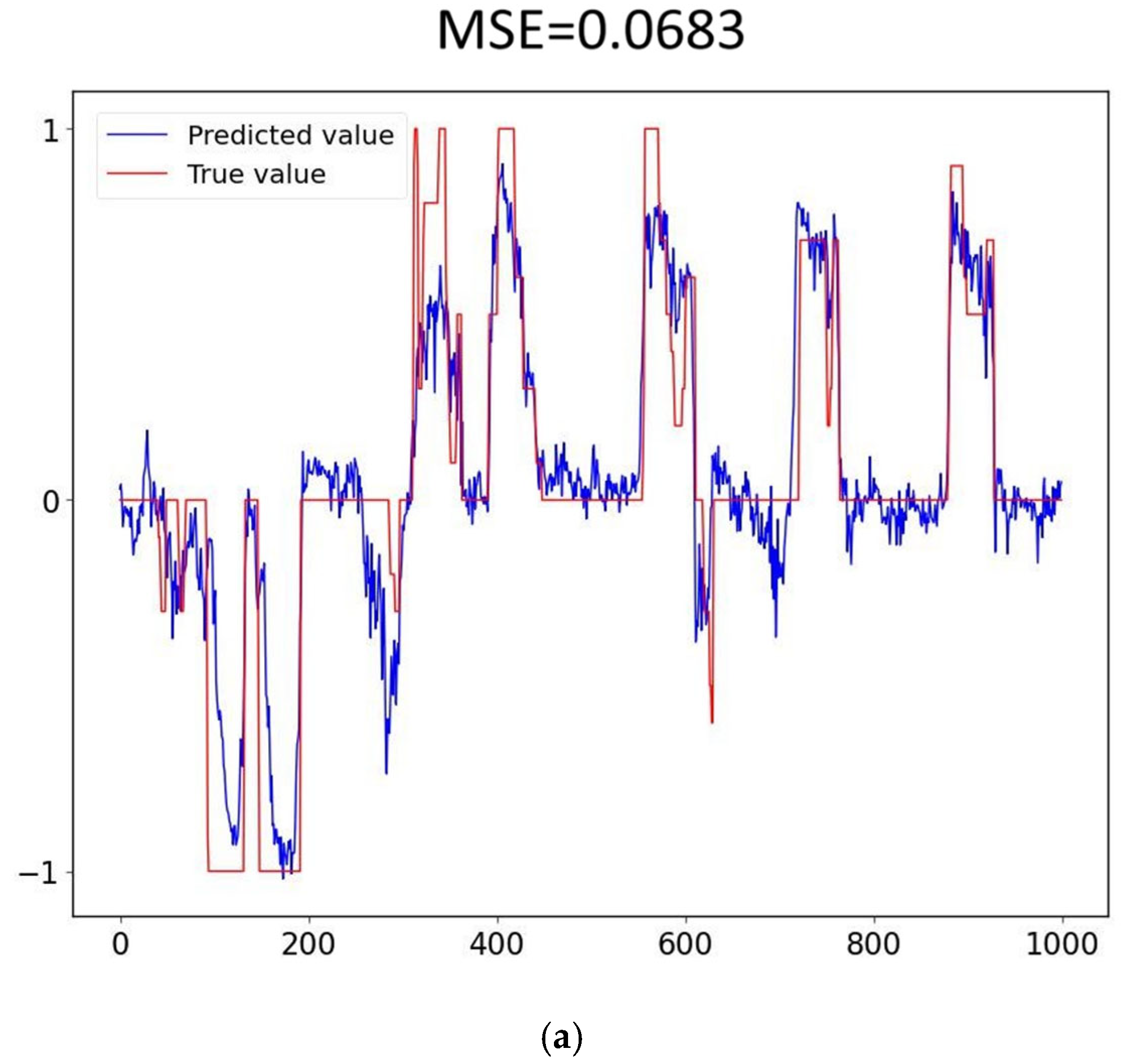
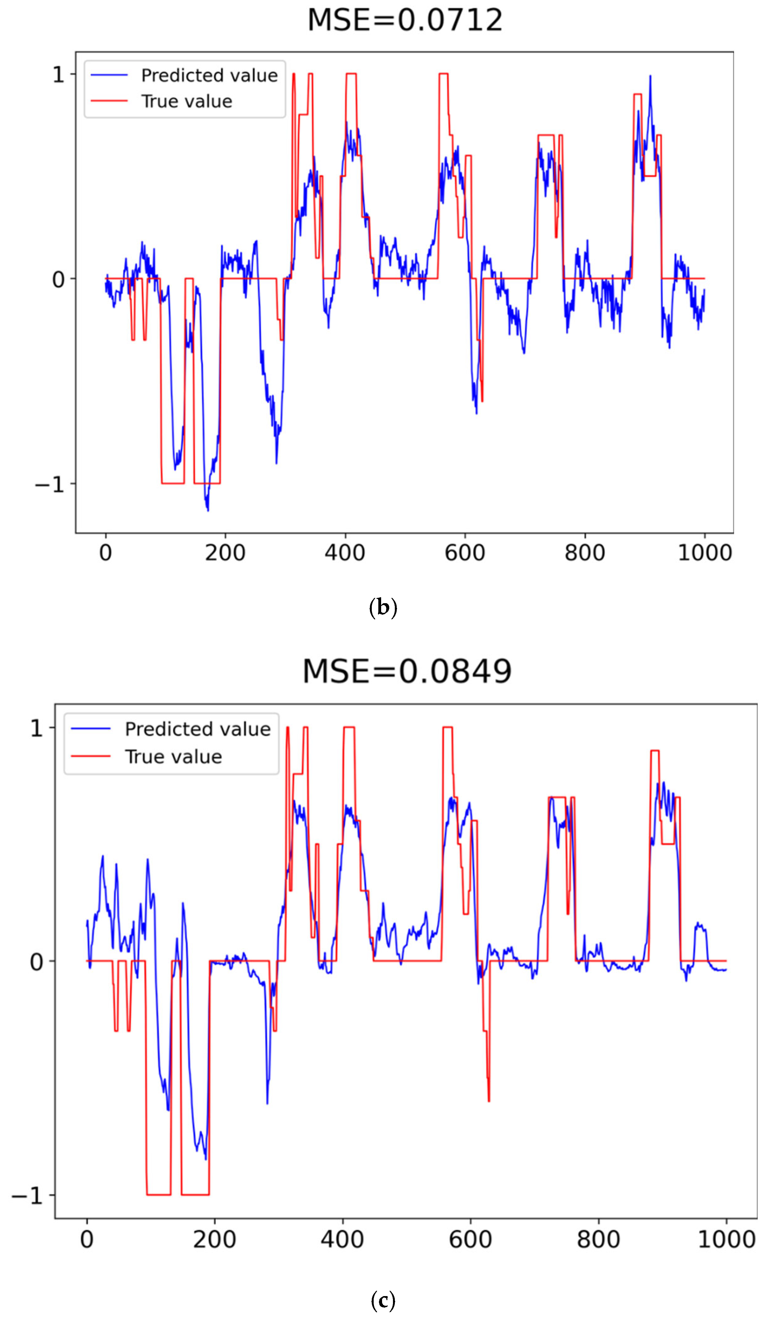
Here, we will evaluate the execution speed and accuracy of every steering angle prediction model. After training the models with the same parameter settings, the experiment tested the trained models with 1000 identical images and plotted the predicted and actual values, as shown in Figure 31. In the test, Equation (2) computes the execution speed FPS, and Equation (4) evaluates the prediction accuracy MSE, as listed in Table 9. In Figure 31, the red line represents the actual steering value, and the blue line is the predicted steering value. We predefined the turning value limited between −1 and 1, where −1 means turn right, 1 means turn left, and 0 means go straight. In Table 9, the LW-ResNet18 model obtains the smallest MSE, and the Nvidia-CNN model achieves the biggest $MSE$.

Figure 31. Predicted and actual values of steering angle prediction model. (a) LW-ResNet18; (b) ResNet18; (c) CNN; (d) Nvidia-CNN.

Table 9. Speed and loss of steering angle prediction models.

Metrics	LW-ResNet18	ResNet18	CNN	Nvidia-CNN
FPS	32.6	27.0	31.9	31.5
MSE	0.0683	0.0712	0.0849	0.0953

4.5. Self-Driving System Assessment

The autonomous driving system adopts the execution speed and the prediction accuracy performed in Jetson Nano as the evaluation indicator. When JetRacer starts self-driving on the road map, the autonomous driving system must simultaneously implement real-time object detection and steering angle prediction. Therefore, the execution speed of object detection is probably the most critical consideration because taking longer to detect objects will endanger self-driving due to the lack of time to complete steering angle prediction. The execution speed is frames per second (FPS) of object detection in a specific model. The object detection model can use TensorRT to accelerate and significantly improve the inference speed of the deep learning model.

First, based on Equation (2), Table 10 lists the frame rate calculation of several integration systems in which Jetson Nano can operate at a resolution of 224 × 224 per frame. As a result, the YOLOv4-tiny model can achieve the best execution speed on average among the integration systems. Integrating LW-YOLOv4-tiny and CNN models can obtain the best execution speed, and integrating YOLOv7 and ResNet18 can obtain the least.

Table 10. FPS of integrated models.

	O. D.	LW-YOLOv4-Tiny	YOLOv4-Tiny	YOLOv5s	YOLOv5n	YOLOv7	YOLOv7-Tiny
St. A. P.
Nvidia-CNN		20.4	19.5	15.6	18.1	10.8	19.0
CNN		20.6	19.6	15.8	18.2	11.0	19.1
ResNet18		18.9	18.4	14.5	17.1	9.7	17.8
LW-ResNet18		19.4	18.9	15.1	17.8	10.5	18.6
Average		19.8	19.1	15.3	17.8	10.5	18.6

O. D.: object detection, and St. A. P.: steering angle prediction.

Next, we focused on both the precision of object detection and the accuracy of the steering angle prediction model, the models of which run on Jetson Nano. Based on Equations (3) and (4), we can calculate the precision of object detection and the accuracy of steering angle prediction under the 224 × 224 resolution image per frame, as listed in Table 11. In Table 11, the YOLOv5s model can achieve the best object detection precision, and the LW-ResNet18 model can obtain the lowest loss of steering angle prediction in the autonomous driving system.

Table 11. The accuracy of integrated models.

	Precision (%)	O. D.
MSE		LW-YOLOv4-Tiny	YOLOv4-Tiny	YOLOv5s	YOLOv5n	YOLOv7	YOLOv7-Tiny
St. A. P.	Nvidia-CNN	(0.0953, 97.3)	(0.0953, 97.2)	(0.0953, 99.1)	(0.0953, 97.7)	(0.0953, 98.9)	(0.0953, 97.0)
	CNN	(0.0849, 97.3)	(0.0849, 97.2)	(0.0849, 99.1)	(0.0849, 97.7)	(0.0849, 98.9)	(0.0849, 97.0)
	ResNet18	(0.0712, 97.3)	(0.0849, 97.2)	(0.0849, 99.1)	(0.0849, 97.7,)	(0.0849, 98.9)	(0.0849, 97.0)
	LW-ResNet18	(0.0683, 97.3)	(0.0849, 97.2)	(0.0849, 99.1)	(0.0849, 97.7)	(0.0849, 98.9)	(0.0849, 97.0)

The first number within a parenthesis represents the steering angle prediction loss (MSE), and the second stands for the object detection precision (%). O. D.: object detection, and St. A. P.: steering angle prediction.

4.6. Performance Indicator

By maintaining the high object detection accuracy in the autonomous driving system, the integrated model can perform a higher frame rate FPS, which evaluates the performance indicator. The baseline is the integrated model with the lowest frame rate performance. Equation (5) calculates the FPS ratio (FR) of an integrated model out of various combinations, where $m$ is the $m$th integrated model, $M$ indicates the number of integrated models, $FP{S}_m$ represents the FPS of the $m$th integrated model, $LS$ stands for the lowest FPS out of integrated models, and $F{R}_m$ denotes FR of the $m$th integrated model.

$$F{R}_m=\frac{FP{S}_m}{LS}, where m=1, 2,\dots , M$$

(5)

Table 12 lists the FR of various integrated models. The FR of integrated YOLOv7 and ResNet18 models is 1, and the lowest FR is based on Equation (5). In Table 12, regarding the execution FPS ratio, the object detection model LW-YOLOv4-tiny can achieve the best average FR, and YOLOv7 is the least.

Table 12. FR of Integrated Models.

	O. D.	LW-YOLOv4-Tiny	YOLOv4-Tiny	YOLOv5s	YOLOv5n	YOLOv7	YOLOv7-Tiny
St. A. P.
Nvidia-CNN		2.1031	2.0103	1.6082	1.8660	1.1134	1.9588
CNN		2.1237	2.0206	1.6289	1.8763	1.1340	1.9691
ResNet18		1.9485	1.8969	1.4948	1.7629	1.0000	1.8351
LW-ResNet18		2.0000	1.9485	1.5567	1.8351	1.0825	1.9175
Average		2.0438	1.9691	1.5722	1.8351	1.0825	1.9201

O. D.: object detection, and St. A. P.: steering angle prediction.

The above analysis considers only the FR of various integrated models. The prediction accuracy between object detection and steering angle prediction is also vital for the autonomous driving system. Equation (6) calculates the precision ratio of object detection (ODPR), where $n$ is the $n$th object detection model, $N$ indicates the number of object detection models, $mA{P}_n$ represents the mAP of the $n$th object detection model, $LmA{P}_n$ stands for the lowest mAP among the object detection models, and $ODP{R}_n$ denotes the precision ratio of the $n$th object detection model.

$$ODP{R}_n=\frac{mA{P}_n}{LmA{P}_n}, where n=1, 2,\dots , N$$

(6)

Equation (7) calculates the loss ratio of the steering angle prediction (SAPLR), where $o$ is the $o$th steering angle prediction model, $O$ indicates the number of steering angle prediction models, $MS{E}_o$ represents MSE of the $o$th steering angle prediction model, $LMSE$ stands for the lowest loss among steering angle prediction models, and $SAPL{R}_o$ denotes the SAPLR of the $o$th steering angle prediction model.

$$SAPL{R}_o=\frac{LMSE}{MS{E}_o}, where o=1, 2,\dots , O$$

(7)

Equation (8) calculates the precision ratio of an integrated model (PR) out of various combinations, where $p$ is the $p$th integrated model, $P$ indicates the number of integrated models, $ODP{R}_p$ represents ODPR of the $p$th integrated model, $SAPL{R}_p$ stands for the SAPLR of the $p$th integrated model, and $P{R}_p$ denotes PR of the $p$th integrated model.

$$P{R}_p=ODP{R}_p\times SAPP{R}_p, where p=1, 2,\dots , P$$

(8)

Table 13 lists the PR of various integrated models. The PR of integrated YOLOv7-tiny and Nvidia-CNN models is 1, and the lowest PR is based on Equation (8). In Table 13, regarding the predictive precision ratio, the steering angle prediction model LW-ResNet18 can achieve the best average PR, and Nvidia-CNN is the least.

Table 13. PR of Integrated Models.

	O. D.	LW-YOLOv4-Tiny	YOLOv4-Tiny	YOLOv5s	YOLOv5n	YOLOv7	YOLOv7-Tiny	Average
St. A. P.
Nvidia-CNN		1.0031	1.0021	1.0216	1.0072	1.0196	1.0000	1.0089
CNN		1.1260	1.1248	1.1468	1.1306	1.1445	1.1225	1.1325
ResNet18		1.3426	1.3412	1.3674	1.3481	1.3647	1.3385	1.3504
LW-ResNet18		1.3996	1.3982	1.4255	1.4054	1.4226	1.3953	1.4078

O. D.: object detection, and St. A. P.: steering angle prediction.

Furthermore, Equation (9) calculates the primitive performance indicator (PPI), that is, FR multiplied by PR, where $q$ is of the $q$th integration system; $m$ indicates the $m$th integration system; $p$ shows the $p$th integration system; $Q$, $M$, and $P$ are the number of integration systems; $F{R}_m$ represents the FP of the $m$th integration system; $P{R}_p$ stands for the PR of the $p$th integration system; and $PP{I}_q$ denotes the PPI of the $q$th integration system.

$$PP{I}_q=F{R}_m\times P{R}_p, where q=1,2,\dots ,Q, m=1,2,\dots , M, p=1,2,\dots , P$$

(9)

Table 14 lists the PPI of various integrated models. Based on Equation (9), the integrated YOLOv7 and Nvidia-CNN models have the lowest PPI, and the integrated LW-YOLOv4-tiny and LW-ResNet18 models have the best PPI. In Table 14, the object detection model LW-YOLOv4-tiny can achieve the best average PPI, and the steering angle prediction model LW-ResNet18 can obtain the highest PPI on average.

Table 14. PPI of Integrated Models.

	O. D.	LW-YOLOv4-Tiny	Yolov4-Tiny	YOLOv5s	YOLOv5n	YOLOv7	YOLOv7-Tiny	Average
St. A. P.
Nvidia-CNN		2.1096	2.0145	1.6429	1.8794	1.1352	1.9588	1.7901
CNN		2.3913	2.2728	1.8680	2.1213	1.2979	2.2103	2.0269
ResNet18		2.6161	2.5441	2.0440	2.3766	1.3647	2.4563	2.2336
LW- ResNet18		2.7992	2.7244	2.2191	2.5790	1.5400	2.6755	2.4229
Average		2.4790	2.3890	1.9435	2.2391	1.3344	2.3252

O. D.: object detection, and St. A. P.: steering angle prediction.

Finally, Equation (10) calculates performance indicator (PI), which is the ratio of the PPI to the lowest PPI among the integrated models, where $r$ is the $r$th integrated model, $R$ indicates the number of integrated models, $PP{I}_r$ represents PPI of the $r$th integrated model, $LPP{I}_r$ stands for the lowest PPI among the integrated models, and $P{I}_r$ denotes PI of the $r$th integrated model.

$$P{I}_r=\frac{PP{I}_r}{LPP{I}_r}, where r=1,2,\dots ,R$$

(10)

Table 15 lists the PI of various integrated models. Based on Equation (10), the integrated YOLOv7 and Nvidia-CNN models have the lowest PI, and the integrated LW-YOLOv4-tiny and LW-ResNet18 models have the best PI. In Table 15, the object detection model LW-YOLOv4-tiny can achieve the best average PI, and the steering angle prediction model LW-ResNet18 can obtain the highest PPI on average.

Table 15. PI of Integrated Models.

	O. D.	LW-YOLOv4-Tiny	YOLOv4-Tiny	YOLOv5s	YOLOv5n	YOLOv7	YOLOv7-Tiny	Average
St. A. P.
Nvidia-CNN		1.8584	1.7746	1.4472	1.6556	1.0000	1.7255	1.5769
CNN		2.1065	2.0021	1.6455	1.8687	1.1433	1.9471	1.7855
ResNet18		2.3045	2.2411	1.8006	2.0936	1.2022	2.1638	1.9676
LW-ResNet18		2.4658	2.3999	1.9548	2.2718	1.3566	2.3569	2.1343
Average		2.1838	2.1044	1.7120	1.9724	1.1755	2.0483

O. D.: object detection, and St. A. P.: steering angle prediction.

4.7. Discussion

In the vision-based autonomous driving system, the proposed approach compares with the method introduced by Bojarski et al. [8], which proposed the other two classical convolutional neural networks. This study tested several models used in steering angle prediction: Nvidia-CNN, traditional CNN, ResNet18, and LW-ResNet18. As per the results, LW-ResNet18 can achieve the best precision of steering angle prediction. On the contrary, the traditional CNN can achieve a better inference speed for steering angle prediction. Duong et al. [9] simulated autonomous driving on the virtual UDACITY platform.

In contrast, the proposed autonomous driving system is implemented on a small-size model car. Several studies [10,11,12] used Raspberry Pi as the computing platform to run the autonomous driving system. Nevertheless, this study applied Jetson Nano with powerful functions to implement the autonomous driving system. In addition, we proposed the integration system to perform object detection and steering angle prediction simultaneously.

For the object detection task, we tested several different models, namely, LW-YOLOv4-tiny, YOLOv4-tiny, YOLOv5s, YOLOv5n, YOLOv7, and YOLOv7-tiny, in this study. Although the YOLOv5s and the YOLOv7 models can achieve higher accuracies of 99.1% and 98.9%, respectively, the inference speed by FPS of YOLOv5s and the YOLOv7 models is much slower than that of the LW-YOLOv4-tiny model in the object detection. Both later models decrease the response time to object detection due to lower FPS and, thus, delay self-driving steering angle prediction. As a consequence, they can induce unsafe driving in autonomous driving systems. Therefore, the object detection accuracy of autonomous driving is not the most critical factor affecting safe driving. Instead, in the autonomous driving system, the most critical factor for safe driving is seeking the highest inference speed by FPS without sacrificing the recognition precision and integrating a high-precision steering angle prediction model with the lowest response time. As a result, integrating the object detection model LW-YOLOv4-tiny and the steering angle prediction model LW-ResNet18 can obtain the best performance index in the experiments.

Due to the limited hardware performance of Jetson Nano, the performance of the autonomous driving system in JetRacer is characterized by a trade-off between the FPS and the accuracy of object detection. We may replace the embedded platform Jetson Nano with Jetson Xavier NX to enhance the execution speed of FPS. Jetson Xavier NX requires more power supply to run the autonomous driving system. However, the model car JetRacer cannot provide enough battery power for Jetson Xavier NX. In other words, the model car JetRacer can adopt Jetson Nano as its embedded platform, which is another limitation.

Moreover, the cameras installed on JetRacer do not have high-resolution image quality. Therefore, the video captured from the camera is unclear when JetRacer is self-driving. Therefore, we are seeking high-resolution cameras to capture video with better image quality in the future.

5. Conclusions

If an autonomous driving system cannot respond fast to driving control appropriately, it will cause high-risk problems with regard to severe car accidents in self-driving. This study proposes the vision-based integration of LW-YOLOv4-tiny and LW-ResNet18 models to real-time fuse the information about rapid object detection and rapid steering angle prediction for safe self-driving. The proposed approach uses ghost convolutions instead of a traditional one, thus shorting the response time of inference intuitively without scarifying the recognition precision. The performance evaluation shows that the proposed approach can outperform the other alternatives.

In future work, we will introduce a LiDAR sensor for the autonomous driving model car, allowing real-time self-positioning in an open space. LiDAR sensors can establish a complete high-precision point cloud map to achieve environmental awareness. With the high-precision positioning in the map, the autonomous driving model car can perform path planning to implement navigation on the road. Furthermore, we will adopt the ROS system combining LiDAR sensors and vision algorithms to effectively run the task of an autonomous driving system in real time. In other words, the ROS system uses a LiDAR sensor to locate traffic signs and visual algorithms to quickly detect and recognize traffic signs and lane lines simultaneously. In such a way, incorporating LiDAR and ROS into an autonomous driving system can significantly enhance safe driving. Furthermore, enlarging the size of a dataset will reduce the gap between the training loss curve and the validation loss curve. The generalization of the model will be better when the separation is relatively small.

References

1. Wang, C.Y.; Bochkovskiy, A.; Liao, H.Y.M. Scaled-Yolov4: Scaling Cross Stage Partial Network. In Proceedings of the IEEE/CVF Conference on Computer Vision and Pattern Recognition, Nashville, TN, USA, 20–25 June 2021; pp. 13029–13038. [Google Scholar]
2. Bochkovskiy, A.; Wang, C.Y.; Liao, H.Y.M. Yolov4: Optimal Speed and Accuracy of Object Detection. arXiv 2020, arXiv:2004.10934. [Google Scholar]
3. He, K.; Zhang, X.; Ren, S.; Sun, J. Deep Residual Learning for Image Recognition. In Proceedings of the IEEE/CVF Conference on Computer Vision and Pattern Recognition, Las Vegas, NV, USA, 27–30 June 2016; pp. 770–778. [Google Scholar]
4. Zhang, G.; Geng, L.; Chen, X. Sound Source Localization Method Based on Densely Connected Convolutional Neural Network. In Proceedings of the 2022 5th International Conference on Information Communication and Signal Processing (ICICSP), Shenzhen, China, 26–28 November 2022; pp. 743–747. [Google Scholar]
5. Waveshare Wiki. JetRacer AI Kit. Available online: https://www.waveshare.com/wiki/JetRacer_AI_Kit (accessed on 1 May 2023).
6. NVIDIA. Jetson Nano Developer Kit. Available online: https://www.nvidia.com/en-us/autonomous-machines/embedded-systems/jetson-nano/ (accessed on 1 May 2023).
7. NVIDIA. TensorRT. 2021. Available online: https://developer.nvidia.com/tensorrt (accessed on 1 May 2023).
8. Bojarski, M.; Testa, D.W.; Dworakowski, D.; Firner, B.; Flepp, B.; Goyal, P.; Jackel, L.D.; Monfort, M.; Muller, U.; Zhang, J.; et al. End to End Learning for Self-Driving Cars. arXiv 2016, arXiv:1604.07316. [Google Scholar]
9. Duong, M.T.; Do, T.D.; Le, M.H. Navigating Self-Driving Vehicles Using Convolutional Neural Network. In Proceedings of the 4th IEEE International Conference on Green Technology and Sustainable Development, Ho Chi Minh City, Vietnam, 23–24 November 2018; pp. 607–610. [Google Scholar]
10. Do, T.D.; Duong, M.; Dang, T.Q.V.; Le, M.H. Real-Time Self-Driving Car Navigation Using Deep Neural Network. In Proceedings of the 4th IEEE International Conference on Green Technology and Sustainable Development, Ho Chi Minh City, Vietnam, 23–24 November 2018; pp. 7–12. [Google Scholar]
11. Jain, A.K. Working Model of Self-Driving Car Using Convolutional Neural Network, Raspberry Pi, and Arduino. In Proceedings of the Second IEEE International Conference on Electronics, Communication and Aerospace Technology, Coimbatore, India, 29–31 March 2018; pp. 1630–1635. [Google Scholar]
12. Seth, A.; James, A.; Mukhopadhyay, S.C. 1/10th Scale Autonomous Vehicle Based on Convolutional Neural Network. Int. J. Smart Sens. Intell. Syst. 2020, 13, 1–17. [Google Scholar] [CrossRef]
13. Omrane, H.; Masmoudi, M.S.; Masmoudi, M. Neural Controller of Autonomous Driving Mobile Robot by An Embedded Camera. In Proceedings of the 4th IEEE International Conference on Advanced Technologies for Signal and Image Processing, Sousse, Tunisia, 21–24 March 2018; pp. 1–5. [Google Scholar]
14. Simmons, B.; Adwani, P.; Pham, H.; Alhuthaifi, Y.; Wolek, A. Training a Remote-Control Car to Autonomously Lane-Follow Using End-to-End Neural Networks. In Proceedings of the 3rd IEEE Annual Conference on Information Sciences and Systems, Baltimore, MD, USA, 20–22 March 2019; pp. 1–6. [Google Scholar]
15. Karni, U.; Ramachandran, S.S.; Sivaraman, K.; Veeraraghavan, A.K. Development of Autonomous Downscaled Model Car Using Neural Networks and Machine Learning. In Proceedings of the 3rd IEEE International Conference on Computing Methodologies and Communication, Erode, India, 27–29 March 2019; pp. 1089–1094. [Google Scholar]
16. Redmon, J.; Farhadi, A. Yolov3: An Incremental Improvement. arXiv 2018, arXiv:1804.02767. [Google Scholar]
17. Yun, S.; Han, D.; Oh, S.J.; Chun, S.; Choe, J.; Yoo, Y. Cutmix: Regularization Strategy to Train Strong Classifiers with Localizable Features. In Proceedings of the IEEE/CVF International Conference on Computer Vision, Seoul, Republic of Korea, 27 October–2 November 2019; pp. 6023–6032. [Google Scholar]
18. Ghiasi, G.; Lin, T.Y.; Le, Q.V. DropBlock: A Regularization Method for Convolutional Networks. In Proceedings of the 32nd International Conference on Neural Information Processing Systems, Red Hook, NY, USA, 3 December 2018; pp. 10750–10760. [Google Scholar]
19. Müller, R.; Kornblith, S.; Hinton, G.E. When Does Label Smoothing Help? arXiv 2019, arXiv:1906.02629. [Google Scholar]
20. Misra, D. Mish: A Self Regularized Non-Monotonic Neural Activation Function. arXiv 2019, arXiv:1908.08681. [Google Scholar]
21. Wang, C.Y.; Liao, H.Y.M.; Wu, Y.H.; Chen, P.Y.; Hsieh, J.W.; Yeh, I.H. CSPNet: A new backbone that can enhance learning capability of CNN. In Proceedings of the IEEE/CVF Conference on Computer Vision and Pattern Recognition, Seattle, WA, USA, 13–20 June 2020; pp. 390–391. [Google Scholar]
22. Zheng, Z.; Wang, P.; Ren, D.; Liu, W.; Ye, R.; Hu, Q.; Zuo, W. Enhancing Geometric Factors in Model Learning and Inference for Object Detection and Instance Segmentation. IEEE Trans. Cybern. 2021, 52, 8574–8586. [Google Scholar] [CrossRef] [PubMed]
23. Woo, S.; Park, J.; Lee, J.Y.; Kweon, I.S. CBAM: Convolutional block attention module. In Proceedings of the European Conference on Computer Vision, Munich, Germany, 8–14 September 2018; pp. 3–19. [Google Scholar]
24. Jocher, G.; Stoken, A.; Borovec, J.; Changyu, L.; Hogan, A.; Diaconu, L.; Ingham, F.; Poznanski, J.; Fang, J.; Yu, L. Ultralytics/Yolov5: v3.1-Bug Fixes and Performance Improvements. 2020. Available online: https://zenodo.org/record/4154370#.ZFjQp3ZByUk (accessed on 1 May 2023).
25. He, K.; Zhang, X.; Ren, S.; Sun, J. Spatial Pyramid Pooling in Deep Convolutional Networks for Visual Recognition. IEEE Trans. Pattern Anal. Mach. Intell. 2015, 37, 1904–1916. [Google Scholar] [CrossRef] [PubMed]
26. Wang, C.Y.; Bochkovskiy, A.; Liao, H.Y.M. YOLOv7: Trainable Bag-of-Freebies Sets New State-of-The-Art for Real-Time Object Detectors. arXiv 2022, arXiv:2207.02696. [Google Scholar]
27. Neupane, D.; Kim, Y.; Seok, J. Bearing Fault Detection Using Scalogram and Switchable Normalization-Based CNN (SN-CNN). IEEE Access 2021, 9, 88151–88166. [Google Scholar] [CrossRef]
28. Han, K.; Wang, Y.; Tian, Q.; Guo, J.; Xu, C.; Xu, C. Ghostnet: More Features from Cheap Operations. In Proceedings of the IEEE/CVF Conference on Computer Vision and Pattern Recognition, Seattle, WA, USA, 13–20 June 2020; pp. 1580–1589. [Google Scholar]
29. He, K.; Sun, J. Convolutional Neural Networks at Constrained Time Cost. In Proceedings of the IEEE Conference on Computer Vision and Pattern Recognition (CVPR), Boston, MA, USA, 7–12 June 2015; p. 5354. [Google Scholar]
30. Jocher, G.; Stoken, A.; Chaurasia, A.; Borovec, J.; Kwon, Y.; Michael, K.; Skalski, S.P. ultralytics/yolov5: v6.0-YOLOv5n ‘Nano’ Models, Roboflow Integration, TensorFlow Export, OpenCV DNN Support. 2021. Available online: https://zenodo.org/record/5563715#.ZFn7fc5ByUk (accessed on 1 May 2023). [CrossRef]
31. LeCun, Y.; Boser, B.; Denker, J.S.; Henderson, D.; Howard, R.E.; Hubbard, W.; Jackel, L.D. Backpropagation Applied to Handwritten Zip Code Recognition. Neural Comput. 1989, 1, 541–551. [Google Scholar] [CrossRef]
Disclaimer/Publisher’s Note: The statements, opinions and data contained in all publications are solely those of the individual author(s) and contributor(s) and not of MDPI and/or the editor(s). MDPI and/or the editor(s) disclaim responsibility for any injury to people or property resulting from any ideas, methods, instructions or products referred to in the content.
Article Metrics
Citations
Article Access Statistics
Multiple requests from the same IP address are counted as one view.