A System-Level Performance Evaluation for a 5G System under a Leaky Coaxial Cable MIMO Channel for High-Speed Trains in the Railway Tunnel

Abstract

As one of the typical application scenarios in the fifth generation (5G) mobile communication system, the situation of high-speed mobile communication is receiving increasing attention. The railway tunnel is a typical environment for high-speed mobile communications. Railway tunnels for high-speed trains are generally installed with leaky coaxial cables (LCXs), which can radiate and receive electromagnetic waves through slots; thus, providing communication. To evaluate the system-level performance of the LCX channel in a tunnel, we propose a modified geometrically based single-bounce multiple-input-multiple-output (GBSB-MIMO) channel model considering the effect of Doppler spread. The time-domain statistics of the channel model are studied from numerical simulations. Based on the proposed channel model, we also simulate and analyze the effects of different factors on the 5G system-level performance, including the interval of cable slots and the quantity and location of LCX.

1. Introduction

Currently, the fifth generation (5G) mobile communication system is being widely used and plays an important role in actual information and communication engineering [1]. Among the many specific scenarios, the high-speed mobile scenario, as a typical application, has attracted increasing attention [2]. In daily life, high-speed railway trains have become one of the main choices for many people to commute or travel, which presents higher requirements for communication quality in this setting. Meanwhile, the high-speed railway communication network still needs to carry the scheduling information to realize efficient high-speed railway network management planning, such as train dispatching information and control data for safety. Therefore, improving the channel capacity of high-speed railway communication systems has gradually become a prominent research topic.

In many specific scenarios of high-speed train operation, the tunnel environment is an urgent problem to be optimized for wireless communication. Due to the relatively closed space of the high-speed railway in the tunnel, the train can only communicate with the transceiver inside the tunnel, which also leads to more reflection, diffraction and scattering in the propagation of wireless signals. Leaky coaxial cables (LCXs) are widely used in railway tunnels. The outer conductor of the LCX is slotted in equal intervals in advance. The electromagnetic wave is radiated on the outside through these slots while transmitting in the LCX, and the external electromagnetic field can also be induced into the LCX through slots and is transmitted to the receiver. Therefore, LCX has the dual functions of transmitting and receiving electromagnetic waves, which can provide uniform and stable signal coverage to improve the quality of wireless communication in tunnel environments.

The channel model of LCXs has been examined in many studies. In [3,4], the transmission and radiation characteristics of LCX with periodic slots are described with the introduction of the electric field transmission on the LCX surface and its space distribution, which form a basis for the calculation and analysis of the radiation field of LCX. In [5], complete simulations on electromagnetic characteristics of the LCX are made for visualizing the radiation field of the LCX and clarifying its impact on the system. In [6,7], the electric field radiation distribution of slotted LCX in the railway tunnel is calculated, which provides a reference for the time-domain response of the LCX channel in the tunnel. With experimental tests, it is shown that the LCX-MIMO channel can achieve a good channel matrix condition number [8] and coverage performance [9,10,11,12]. In [11,12], it was indicated that the LCX-MIMO system can achieve a larger capacity than that using conventional monopole antennas. In [13], it performs a field measurement of the LCX-MIMO channel in the tunnel and verifies the stability of LCXs used as the radio propagation medium. In [14], it was confirmed that the LCX system can reduce the capacity loss by using position information than that of other systems. For channel modeling, according to the radiation characteristics of LCX in the tunnel, a geometrically-based single-bounce multiple-input-multiple-output (GBSB-MIMO) channel model can be better used to model the LCX channel under the tunnel to simulate the channel statistics and coverage performance [15,16]. Besides, ref. [17] established a channel model based on the state transition method and optimized with the particle swarm optimization (PSO) algorithm. However, most of the literature has not considered the effect of Doppler spread [18]. To evaluate the system-level performance of 5G systems for high-speed trains in the railway tunnel with LCXs, we should study a channel model with the effect of Doppler spread.

In the LCX channel of a railway tunnel, the layout of LCXs and train antenna erection will affect the propagation of wireless signals in the tunnel, further affecting the channel capacity of the LCX channel of the railway tunnel [19]. Considering the actual structure of a railway tunnel, we evaluate the throughput of 5G systems in situations with different LCX patterns. According to the results, we analyze the influence of relevant factors on the LCX channel in turn, which can provide a theoretical reference for the evaluation of the performance of 5G high-speed railway communication systems in tunnels.

The paper is organized as follows: Section 2 introduces the basic composition of the LCX model in the tunnel and the derivation of the channel time-domain response for it, as well as briefly describes the Doppler shift and the modification to the original channel model for its effect. Then, Section 3 mainly discusses the simulation and analysis of the coverage performance of the model’s channel. The results are obtained under the channel model from the perspective of self-statistics and characteristics, as well as the complete throughput system. Finally, Section 4 presents the corresponding analysis conclusions and summary based on the discussion in the previous sections.

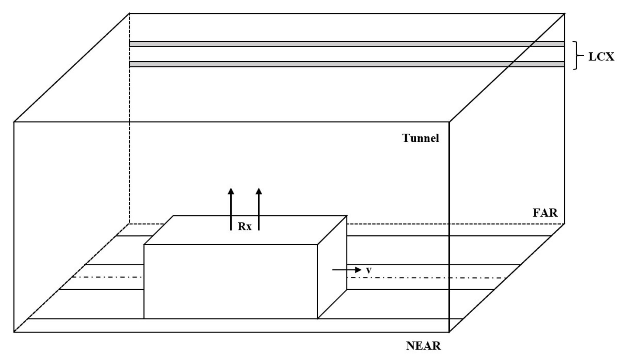
2. The LCX Channel Model in the Tunnel

The LCX tunnel model used for simulation is shown in Figure 1. Considering that the train tunnel often has two-direction carriageways in practice, the train is set symmetrically on the side of the tunnel instead of at the center of the tunnel when established. The transmitter (Tx) and receiver (Rx) consist of LCXs and electric dipoles on the train. As the transmitter, LCXs hang at a certain interval on the sidewall of the tunnel, which is divided into the near side and far side according to the relative position between their sidewall and the train. The receiving antennas are set at the top of the train and arranged along the train direction with a certain interval as the receiver. During simulation, the specific pattern of the model is adjusted according to the quantity of LCXs, the interval between LCXs, the quantity of receiving antennas, etc.

For the analysis of this LCX channel model in tunnels, ref. [16] proposed a geometrically- based single-bounce multiple-input-multiple-output (GBSB-MIMO) channel model. In this model, the time-domain impulse response of the channel can be described as the geometric propagation with a specific transmitter, receiver and scatterer, whose position is defined on the opposite side of the tunnel wall at random according to some probability distributions in advance. Based on the proposed model, we add the consideration of the Doppler shift caused by high-speed movement of the train as a modification. The effect of the Doppler shift is added to the calculation of the channel response to further increase the channel characteristics that can be reflected by the model’s analysis.

For a multiple-input-multiple-output (MIMO) channel, $h_{lp}$ is the time-domain impulse response of the pth transmitting antenna $s_p$ to the lth receiving antenna $r_l$. According to vector symbols $\mathbf{s}={[s_1,s_2,\cdots ,s_p]}^{\prime }$ and $\mathbf{r}={[r_1,r_2,\cdots ,r_l]}^{\prime }$, where ${[·]}^{\prime }$ is the transpose operator, and the input-output equation of the MIMO channel can be expressed as:

$$\mathbf{r}=\mathbf{H}·\mathbf{s}+\mathbf{n}$$

(1)

where H is a complex matrix and ${\left[\mathbf{H}\right]}_{lp}=h_{lp}$. $\mathbf{n}$ is the complex additive white Gaussian noise (AWGN) with a zero mean vector and a diagonal covariance matrix [20].

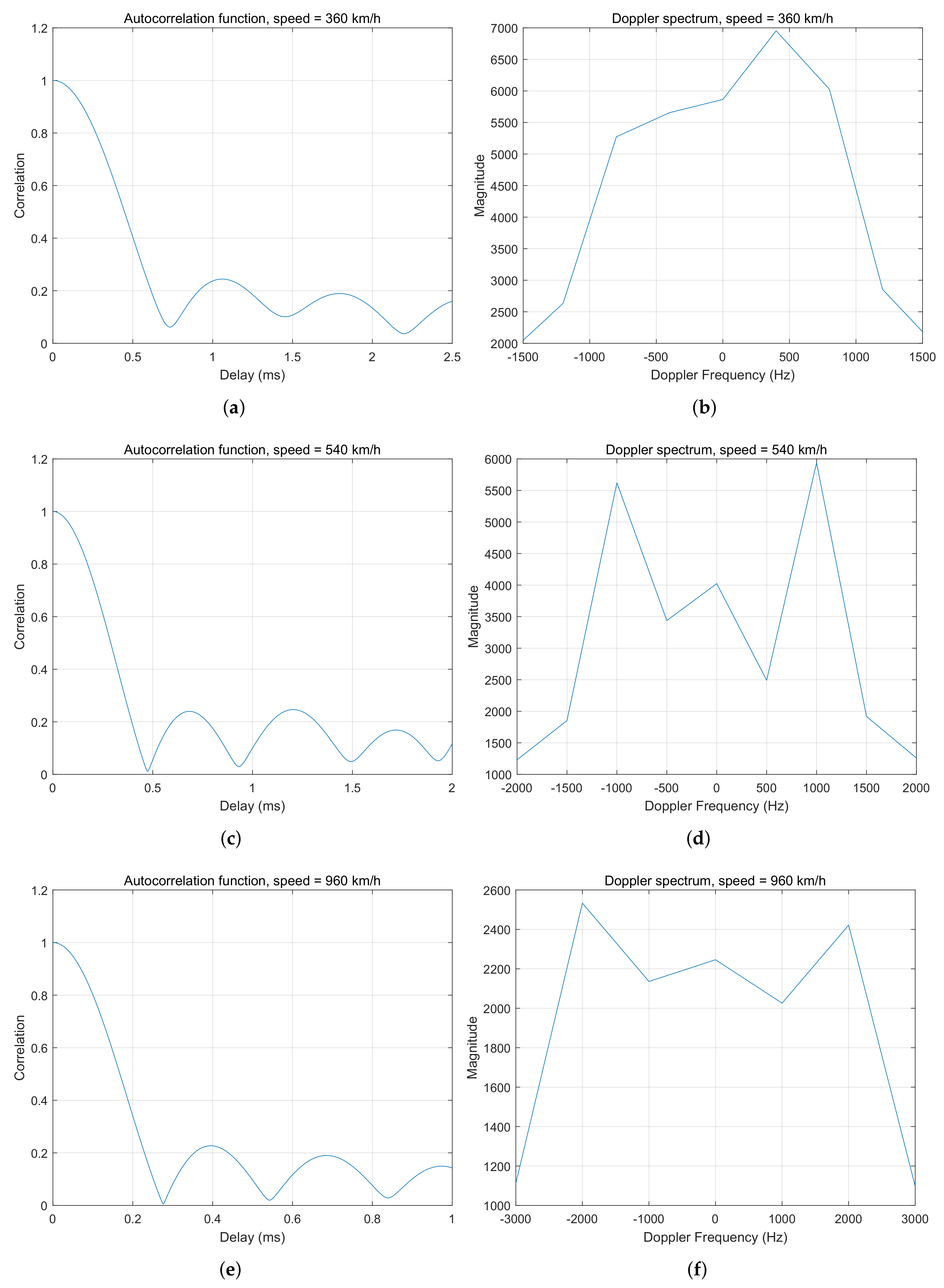
2.1. The Doppler Shift

The fluctuation of the signal in the time domain is closely related to the relative motion between the transmitter and the receiver. This relative motion causes the spread of the signal in the spectrum, which is called the Doppler shift [18]. As shown in Figure 2, the receiving station receiving the signal from the transmitter moves at a constant speed v. The receiving station is at positions $x_1$ and $x_2$ at times $t_1$ and $t_2$, respectively, and the distance between the two positions is d. ${\theta }_1$ and ${\theta }_2$ are the angle between the signal path and the direction of speed v at positions $x_1$ and $x_2$, respectively. When the transmitter is far away from the receiving station, the angle of two positions can be regarded as the same, which can be expressed as ${\theta }_1={\theta }_2=\theta$. Therefore, the difference in distance when the signal is sent by the transmitter is received at positions $x_1$ and $x_2$ is represented as:

$$\Delta l=dcos\theta =v·(t_2-t_1)cos\theta =v·\Delta tcos\theta$$

(2)

At this indent, the phase difference of the received signal caused by the distance difference is expressed as:

$$\Delta \phi =\frac{2\pi \Delta l}{\lambda }$$

(3)

where $\lambda$ is the wavelength of the transmitting signal. Therefore, according to the differential relationship between frequency and phase, the corresponding frequency change, namely, the Doppler frequency, can be obtained. According to (2) and (3), the Doppler frequency can be expressed as:

$$f_d=\frac{1}{2\pi }\frac{\Delta \phi }{\Delta t}=\frac{v}{\lambda }cos\theta .$$

(4)

2.2. Channel Time-Domain Impulse Response and Modification of the Channel Model

It is assumed that the electric-field strength on the surface of the first LCX slot is $E_{01}=1V/m$, and the electric-field strength on the surface of the ith LCX slot $E_{0i}$ satisfies $E_{0i}=E_{01}·{\gamma }_i$, where ${\gamma }_i$ is the longitudinal attenuation factor of the ith LCX slot. ${\gamma }_i$ can be expressed as ${\gamma }_i=e^{-j{\beta }_i}·{\alpha }_i$, where ${\alpha }_i$ is the longitudinal amplitude attenuation and ${\beta }_i$ is the phase variation. For the ith slot, ${\alpha }_i$ and ${\beta }_i$ can be represented with the properties of LCX as:

$${\alpha }_i={10}^{\frac{-\alpha ·P(i-1)}{100\times 20}}$$

(5)

$${\beta }_i=k_{r}P(i-1)$$

(6)

where $\alpha$ is the longitudinal power attenuation constant per 100 m (unit in dB/100 m), $k_r$ is the propagation constant of the electrical wave in the LCX and $k_r=k_0\sqrt{{\epsilon }_r}$, and P is the periodicity of the LCX slots [3].

The propagation of the signal from LCX has the line-of-sight (LOS) component and the non-line-of-sight (NLOS) component. We assume that the quantity of slots on one LCX is N, and the quantity of scatterers is M. According to the distribution of LCX radiation [4,6] and (5) and (6), the two components of the radiation field of LCX can be expressed as:

$$E_z^{LOS}=\sum _{i=1}^N{\alpha }_i\frac{sin\left({\theta }_i\right)}{r_i}{e}^{-\iota \left(k_0{r}_i+{\beta }_i\right)}$$

(7)

$$E_z^{NLOS}=\sum _{i=1}^N\sum _{j=1}^M{\alpha }_i\frac{sin\left({\theta }_{ij}\right)}{r_{ij}^{{}^{\prime }}{r}_{ij}^{{}^{″}}}{e}^{-\iota \left[k_0\left(r_{ij}^{{}^{\prime }}+r_{ij}^{{}^{″}}\right)+{\beta }_i\right]}$$

(8)

where $r_i$ is the distance of the LOS propagation link from the ith slot of LCX to the receiving antenna, $r_{ij}^{{}^{\prime }}$ is the distance of the propagation link from the ith slot of LCX to the jth scatterer, $r_{ij}^{{}^{″}}$ is the distance of the propagation link from the jth scatterer to the receiving antenna, ${\theta }_i^{}$ is the angle between the link from the ith slot of LCX to the receiving antenna and the LCX axis, and ${\theta }_{ij}$ is the angle between the link from the ith slot of LCX to the jth scatterer and the LCX axis. According to the LCX channel model above, we set up a Cartesian coordinate system by defining the top LCX as axis z with a positive direction along the extension of LCX and the first slot of it as the origin. As shown in Figure 3 (example with far-side LCXs), the vertical distance between Tx1 and Tx2 is d, the coordinate of Rx1 is (x, y, z), the vertical height of both Rx1 and Rx2 is h, the distance between Rx1 and Rx2 is D, and the coordinates of the jth scatterer are $S_j(x_{0j},y_{0j},z_{0j})$. Therefore, the relevant parameters of the distance and angle above can be written as:

$$\begin{array}{cc}\hfill sin\left({\theta }_i\right)& =\frac{\sqrt{x^2+y^2}}{\sqrt{x^2+y^2+{\left[z-\left(i-1\right)P\right]}^2}}\hfill \\ \hfill sin\left({\theta }_{ij}\right)& =\frac{\sqrt{x_{0j}^2+y_{0j}^2}}{\sqrt{x_{0j}^2+y_{0j}^2+{\left[z_{0j}-\left(i-1\right)P\right]}^2}}\hfill \end{array}$$

(9)

$$\begin{array}{cc}\hfill r_i& =\sqrt{x^2+y^2+{\left[z-\left(i-1\right)P\right]}^2}\hfill \\ \hfill r_{ij}^{{}^{\prime }}& =\sqrt{x_{0j}^2+y_{0j}^2+{\left[z_{0j}-\left(i-1\right)P\right]}^2}\hfill \\ \hfill r_{ij}^{{}^{″}}& =\sqrt{{\left(x-x_{0j}\right)}^2+{\left(y-y_{0j}\right)}^2+{\left(z-z_{0j}\right)}^2}.\hfill \end{array}$$

(10)

The channel is constructed according to the GBSB-MIMO model and the radiation field distribution of LCX [16]. LCXs hang on one side of the tunnel wall, and effective scatterers are assumed to be omnidirectional ideal reflectors, which are distributed on the wall of the other side. $S_j$ is the jth scatterer on the tunnel wall, the transmitter power is $P_{T_x}$, and the receiver power from $T_{x_p}$ to $R_{x_l}$ is ${\mathsf{\Omega }}_{lp}$, which satisfies ${\mathsf{\Omega }}_{lp}\le P_{T_x}$ and ${\mathsf{\Omega }}_{lp}=E\left[{\left|h_{lp}\right|}^2\right]$. With two components of the propagation link, the time-domain impulse response $h_{lp}$ can be obtained as:

$$h_{lp}=h_{lp}^{LOS}+h_{lp}^{NLOS}$$

(11)

where $h_{lp}^{LOS}$ is certain and $h_{lp}^{NLOS}$ is a random process. Combined with the radiation properties of LCX, electromagnetic (EM) considerations and the GBSB model, the two components can be expressed as:

$$h_{lp}^{LOS}=\sqrt{\frac{K_{lp}·{\mathsf{\Omega }}_{lp}}{K_{lp}+1}}·\underset{N\to \infty }{lim}\frac{1}{\sqrt{N}}\sum _{i=1}^N{g}_{lp,i}^{LOS}{e}^{-\iota \left(k_0{r}_{lp,i}+{\beta }_i\right)}$$

(12)

$$h_{lp}^{NLOS}=\sqrt{\frac{{\mathsf{\Omega }}_{lp}}{K_{lp}+1}}·\underset{\genfrac{}{}{0pt}{}{N\to \infty \hfill }{M\to \infty \hfill }}{lim}\frac{1}{\sqrt{NM}}\sum _{i=1}^N\sum _{j=1}^M{g}_{lp,ij}^{NLOS}{e}^{\iota {\phi }_{ij}}{e}^{-\iota \left[k_0\left(r_{lp,ij}^{{}^{\prime }}+r_{lp,ij}^{{}^{″}}\right)+{\beta }_i\right]}$$

(13)

where $K_{lp}$ is the Rician K-factor of the link from $T_{x_p}$ to $R_{x_l}$ and is defined as the ratio between the LOS component power and the NLOS component power satisfying:

$$K_{lp}=\frac{{\left|h_{lp}^{LOS}\right|}^2}{E\left[{\left|h_{lp}^{NLOS}\right|}^2\right]}.$$

$r_{lp,i}$ is the distance from the ith slot of $T_{x_p}$ to $R_{x_l}$, $r_{lp,ij}^{}$ is the distance from the ith slot of $T_{x_p}$ via the jth scatterer to $R_{x_l}$, ${\left\{{\phi }_{ij}\right\}}_{i,j=1}^{\infty }$ are i.i.d random variables with uniform distributions at [0, 2$\pi$), $g_{lp,i}^{LOS}$ is the normalization amplitude of the LOS wave from the ith slot of $T_{x_p}$ to $R_{x_l}$, and $g_{lp,ij}^{NLOS}$ is the normalization amplitude of the wave scattered through the jth scatterer with the wave link $T_{x_{p,j}}\to S_j\to R_{x_l}$. With (7) and (8), $g_{lp,i}^{LOS}$ and $g_{lp,ij}^{NLOS}$ can be expressed as:

$$g_{lp,i}^{LOS}=\frac{{\alpha }_i\frac{sin\left({\theta }_{lp,i}\right)}{r_{lp,i}}}{\sqrt{N^{-1}{\displaystyle \sum _{i=1}^N}{\left({\alpha }_i\frac{sin\left({\theta }_{lp,i}\right)}{r_{lp,i}}\right)}^2}}$$

(14)

$$g_{lp,ij}^{NLOS}=\frac{{\alpha }_i\frac{sin\left({\theta }_{lp,ij}\right)}{r_{lp,ij}^{{}^{\prime }}{r}_{lp,ij}^{{}^{″}}}}{\sqrt{{\left(NM\right)}^{-1}{\displaystyle \sum _{i=1}^N}{\displaystyle \sum _{j=1}^M}{\left({\alpha }_i\frac{sin\left({\theta }_{lp,ij}\right)}{r_{lp,ij}^{{}^{\prime }}{r}_{lp,ij}^{{}^{″}}}\right)}^2}}.$$

(15)

Then, we consider adding the effect of the Doppler shift caused by the high-speed movement of the train to modify and improve the original model above for the high-speed movement scenario. According to (4), when the train moves along the extension direction of the LCX at a constant speed v, the Doppler frequency of the LOS propagation path from the ith LCX slot can be expressed as:

$$f_{d,i}=\frac{v}{\lambda }cos\left({\varphi }_i\right)$$

(16)

where $\lambda$ is the wavelength of the LCX electric field, and ${\varphi }_i$ is the angle between the link from the ith LCX slot to the receiving antenna and the direction of the train speed (here, it is the same as the LCX extension direction). According to the coordinate shown in Figure 3, cos ${\varphi }_i$ can be expressed as:

$$cos\left({\varphi }_i\right)=-\frac{z-\left(i-1\right)P}{\sqrt{x^2+y^2+{\left[z-\left(i-1\right)P\right]}^2}}$$

(17)

where the negative operator indicates that the value of the Doppler frequency is negative when the train departs from the current slot and it is positive when the train approaches the current slot.

For the NLOS propagation link, assuming that the scatterer positions remain unchanged between two sampling times, the signal sent by the LCX slot will be scattered to the receiving antenna through the same scatterers. Therefore, scatterers can be regarded as equivalent signal sources to obtain a simplified Doppler frequency calculation for the NLOS component as:

$$f_{d,j}=\frac{v}{\lambda }cos\left({\varphi }_j\right)$$

(18)

where ${\varphi }_j$ is the angle between the link from the jth scatterer to the receiving antenna and the direction of the train speed. Similar to the above, cos ${\varphi }_j$ can be expressed as:

$$cos\left({\varphi }_j\right)=-\frac{z-z_{0j}}{\sqrt{{\left(x-x_{0j}\right)}^2+{\left(y-y_{0j}\right)}^2+{\left(z-z_{0j}\right)}^2}}$$

(19)

where the meaning of the negative operator is the same as cos ${\varphi }_i$.

Therefore, according to (16) and (18), the time-domain impulse response of the channel at the nth sampling time in (12) and (13) will be modified as:

$$h_{lp}^{LOS}=\sqrt{\frac{K_{lp}·{\mathsf{\Omega }}_{lp}}{K_{lp}+1}}·\underset{N\to \infty }{lim}\frac{1}{\sqrt{N}}\sum _{i=1}^N{g}_{lp,i}^{LOS}{e}^{-\iota \left(k_0{r}_{lp,i}+{\beta }_i\right)}{e}^{\iota \frac{2\pi }{\lambda }v·n{T}_{s}cos\left({\varphi }_i\right)}$$

(20)

$$h_{lp}^{NLOS}=\sqrt{\frac{{\mathsf{\Omega }}_{lp}}{K_{lp}+1}}·\underset{\genfrac{}{}{0pt}{}{N\to \infty \hfill }{M\to \infty \hfill }}{lim}\frac{1}{\sqrt{NM}}\sum _{i=1}^N\sum _{j=1}^M{g}_{lp,ij}^{NLOS}{e}^{\iota {\phi }_{ij}}{e}^{-\iota \left[k_0\left(r_{lp,ij}^{{}^{\prime }}+r_{lp,ij}^{{}^{″}}\right)+{\beta }_i\right]}{e}^{\iota \frac{2\pi }{\lambda }v·n{T}_{s}cos\left({\varphi }_j\right)}$$

(21)

where $T_s$ is the sampling interval.

3. Simulation and Analyses of the Coverage Performance

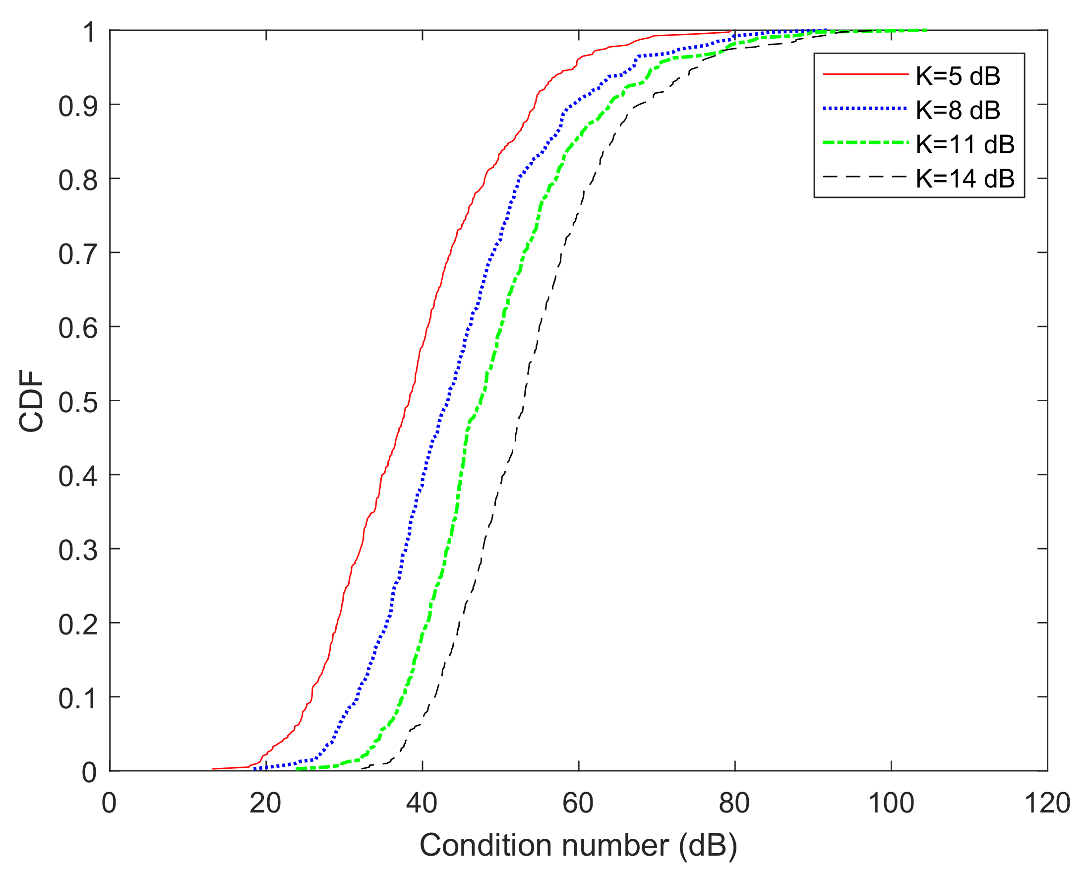
3.1. Condition Number, SINR and Channel Throughput

The condition number (CN) of a MIMO channel matrix can be used to reflect the channel performance [8]. When CN is low, it indicates that MIMO channel conditions are good, which is conducive to the increase of the MIMO system capacity. In contrast, it shows that the MIMO channel has a high correlation, and signals transmitted through the MIMO channel produce large interference when CN is high. The condition number (CN) of the channel matrix is given as:

$$\eta =20{log}_{10}\left({\lambda }_{max}/{\lambda }_{min}\right)$$

(22)

where ${\lambda }_{max}$ and ${\lambda }_{min}$ are the maximum and minimum eigenvalues of the channel matrix, respectively. After obtaining the MIMO channel complex matrix H, the signal-to-interference-plus-noise ratio (SINR) will be calculated as a reference of the maximum coding and modulation rate that can be reached for each data stream at this moment, which can represent the coverage performance of the current channel [8]. The calculation of the SINR is also related to the eigenvalue of the channel matrix as:

$$\mathrm{SINR}\left(dB\right)=10{log}_{10}\left({\lambda }^2·\mathrm{SNR}\right)$$

(23)

where $\lambda$ is the eigenvalue of the channel matrix and SNR is the signal-to-noise ratio. When the position of the train is not far from the starting point, SINR of each data stream is calculated and converted to the corresponding coding and modulation rate, respectively, then the throughput will be obtained by the sum. However, with the train moving, the position of the train is becoming far from the start. Meanwhile, the transmission loss of LCXs will increase and the throughput will have a serious deterioration. In this situation, the system will use the maximum eigenvalue ${\lambda }_{max}$ to make calculations for the transmission of all data streams, which is the maximum eigenmode transmission. At this moment, all data streams will reach the coding and modulation rate correspondingly to the SINR with the maximum eigenvalue of the channel matrix. In this way, the throughput can be compensated and the deterioration of the channel coverage performance will be reduced for the far position of the train.

3.2. Results of the Simulation and Analyses

After modeling the LCX channel for the tunnel, we simulate the characteristics of the channel model, as well as some typical scenarios that it can be applied to. By changing the model composition and parameters for the corresponding scenarios, we analyze the impact on the wireless communication coverage of the tunnel by different LCX quantities (1/2/4), LCX spacings and installed sides of the LCXs. The parameters in the simulation are shown in

Table 1. Parameters in the simulation.

Simulation Information	Downlink
Bandwidth	10 MHz
Frequency of the carrier wave	2.1 GHz
Initial power of each LCX	43 dBm
Noise figure of the receiver	5 dB
Other loss	4 dB
Coupling loss	69 dB
Transmission loss ($\alpha$)	4.7 dB/100 m
Distance of the train on the far side	6.8 m
Height of the train (with receiving antenna)	4.05 m
Distance of the train on the near side	2.2 m
Height of single LCX installation	4.8 m
Height of xth LCX installation	4.8 m − $x\ast \lambda$ (m)
Width Factor	$20{\log }_{10}(TR\_dist/2)$
Interval of slots	0.252 m
System overhead (Plot signal, Cyclic prefix, Signaling⋯)	30%
Maximum modulation order/Spectral efficiency	256QAM/7.4063 bps/Hz
Sampling frequency	15.36 MHz

.

When generating the channel matrix in the simulation, we consider the effect of LCX slots within (−25 m, 25 m) centered on the receiving terminal and set a total of 200 scatterers randomly distributed in this range. In the system simulation, the Rician K-factor is set to 15 dB in the scenario of one or two LCXs on a single side. For the scenario of four LCXs on both sides, the Rician K-factor is set to 15 dB for the near-side LCX and 8 dB for the far-side LCX. SINR will be calculated with the eigenvalues of the channel matrix as a reference to select the rate of coding and modulation for data transmission. When the position of the train is relatively far from the start, the system will use the maximum eigenmode transmission to reduce the deterioration of the channel coverage performance in this situation.

3.2.1. Channel Statistics and Characteristics

First, we simulate and explore the statistics and characteristics of the channel. For example, when applying the system using LCXs on the near side, we select different speeds of train movement and sample the corresponding h11, which is the channel time-domain response between the first LCX and the first receiving antenna. With the samples, we obtain the autocorrelation function and the Doppler spectrum of the LOS and NLOS components of the channel time-domain response to obtain the Doppler characteristics of the channel, as shown in Figure 4 and Figure 5. According to the result, under the LCX model we construct for the tunnel, the channel is approximately presented as a uniform Doppler spectrum for the LOS and NLOS components.

Figure 6 shows the cumulative distribution function of CN for the channel under different Rician K-factors when the system adopts two LCXs on the far side and two receiving antennas. The CN is concentrated near a larger value when the Rician K-factor increases. When combined with the specific meaning of the parameters, the results show that when the Rician K-factor increases, the proportion of the NLOS component to the total power decreases. This intensifies the degree of weak scattering in the channel, which leads to a reduction in channel performance.

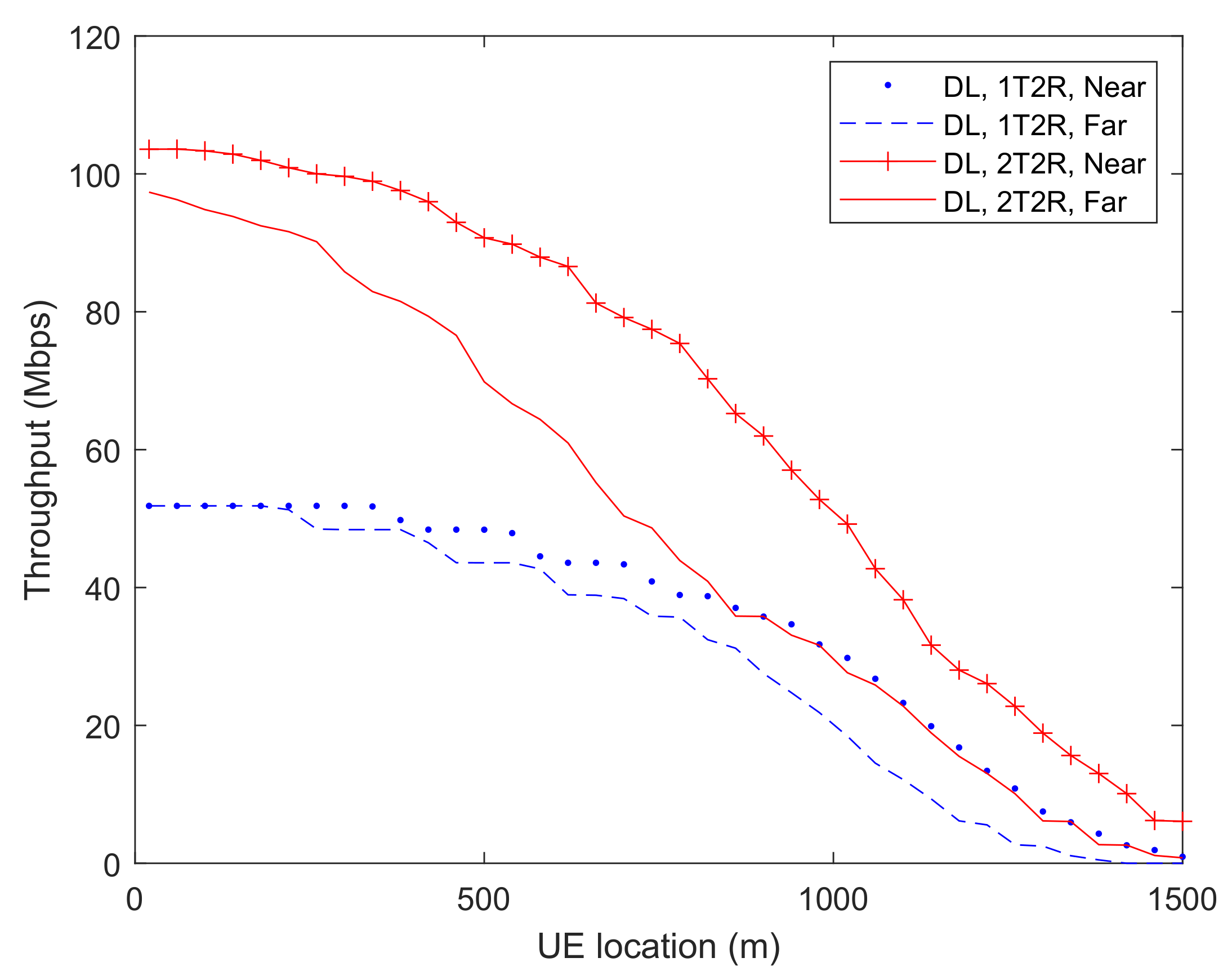
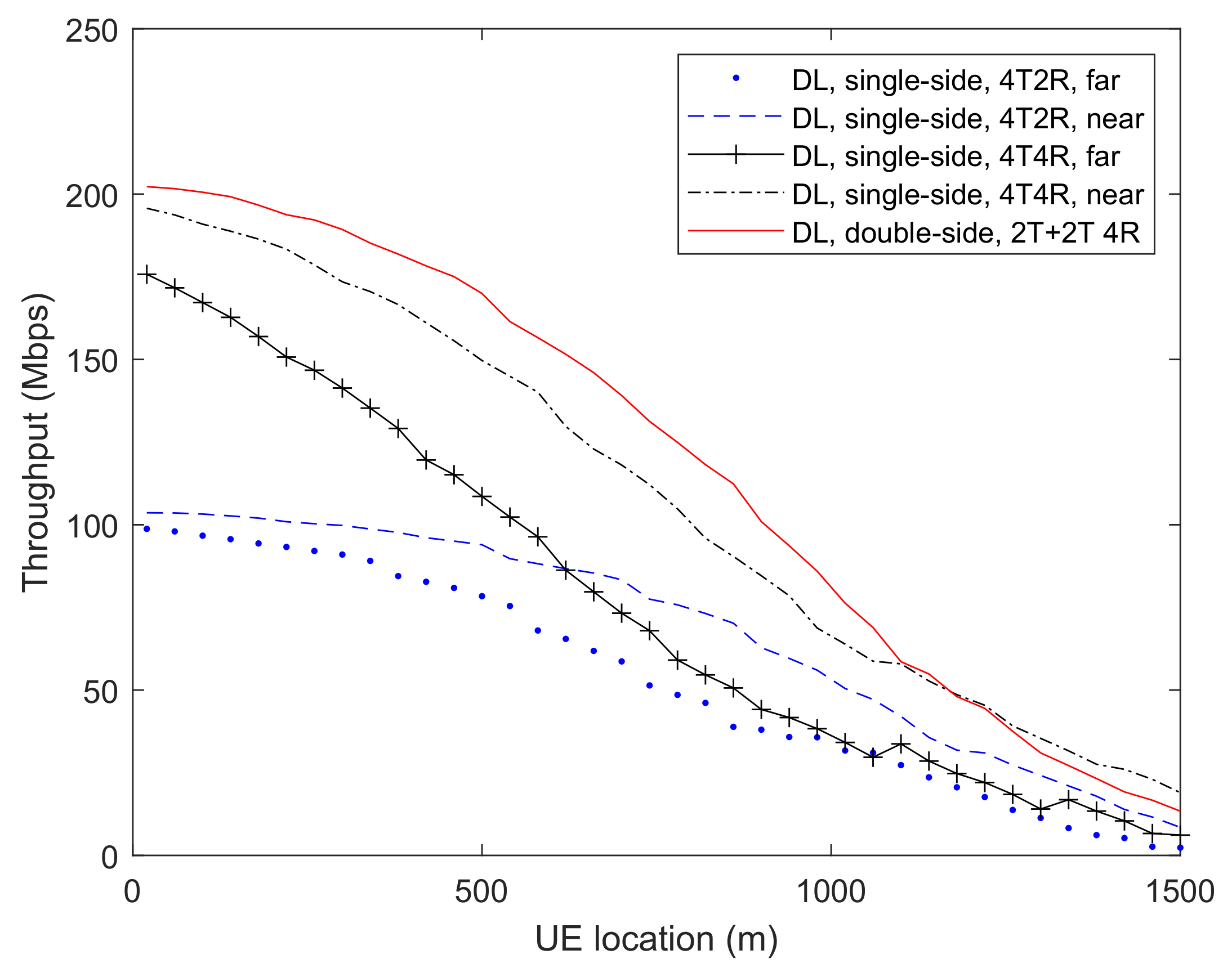
3.2.2. System Simulation for the Throughput

In the system simulation for the throughput, we further simulate the throughput of the LCX channel in different scenarios and analyze the effects of different factors. Figure 7 and Figure 8 show the downlink throughput with different LCX spacing intervals when the system adopts two LCXs and two receiving antennas. LCXs are laid on the near side in Figure 7 and on the far side in Figure 8. It can be seen from the figure that the throughput increases with the increasing LCX spacing interval. After it increases to 4 times the wavelength (4$\lambda$), the throughput continues to increase, but the improvement is small. As shown in Figure 8, when LCXs are laid on the far side, the throughput improvement is not obvious with the increase in the LCX spacing interval. Besides, because the system will use the maximum eigenmode transmission to compensate for the throughput when the train runs to a further position, the gap of the throughput under different parameters will be reduced after a far UE location. Therefore, the curves with different LCX spacing intervals in these two figures will be closer when the value of UE location increases.

Figure 9 shows the downlink throughput with different LCX spacing intervals when the system adopts four LCXs and four receiving antennas. LCXs are symmetrically deployed on both sides of the tunnel, with two LCXs on each side. It can be seen that the throughput also improves with the increase in the LCX spacing interval (>1$\lambda$), but not obviously. Meanwhile, the curves in Figure 9 are also closer in the range of a larger value of the UE location, which is also due to the throughput compensation by the usage of the maximum eigenmode transmission.

Figure 10 shows the downlink throughput when the system adopts one or two LCXs and two receiving antennas. When two LCXs are used, the throughput is considerably improved and has a better performance than when one LCX is used.

Figure 10 shows the downlink throughput when the system adopts four LCXs with different deployments and two or four receiving antennas. The four LCXs can be deployed on both sides or only on one side of the tunnel. For the pattern of LCXs on both sides, LCXs are symmetrically deployed with two LCXs on each side. With a high SNR, the performance of deploying two LCXs on each side is better than deploying four LCXs on one side. This is because when LCXs are deployed on both sides, a better MIMO spatial multiplexing capability can be obtained. When LCXs are wholly deployed on one side, the MIMO spatial multiplexing capability is relatively weak due to the low CN of the channel matrix. Thus, it is better to deploy two LCXs on both sides than four LCXs on one side under a high SNR. However, with a low SNR, deploying four LCXs wholly on the near side can obtain a better throughput performance. However, the performance of the four LCXs wholly on the far side is still worse than that when the LCXs are deployed symmetrically on both sides. Overall, for the pattern of four LCXs, deploying LCXs symmetrically with two on each side can achieve better performance.

In Figure 11, we also compare the situation of two or four receiving antennas. Obviously, the terminal can obtain better performance by using more receiving antennas.

4. Conclusions

In this paper, we consider the effect of the Doppler shift in the GBSB-MIMO channel model in a tunnel with the LCX and perform simulations to obtain some characteristics of the channel model. In addition, we simulate the change in channel throughput with different positions of the train and then change the pattern and composition of the model to analyze the effects of the near and far LCX, the 1/2/4 LCX, the different intervals of the LCX layout of one side and the quantity of receiving antennas on the channel throughput. With the channel modeling and simulation results, we obtain the following conclusions:

(1) In order to indicate the impact of train mobility, we calculate the Doppler shift caused by its velocity into the channel modeling in the railway tunnel. In the modified tunnel model, the time domain responses of the LOS and NLOS components approximately have the statistics of a uniform Doppler spectrum.

(2) When LCXs are laid on the near side, the increase in the interval between LCXs can improve the channel throughput. When the interval is increased to 4 times the wavelength (4$\lambda$), the improvement degree decreases. When LCXs are laid on the far side or on both sides, the increment of the LCX interval (>1$\lambda$) does not considerably improve the channel capacity.

(3) When two LCXs are laid on one side, the channel throughput is substantially better than that when only one LCX is laid on one side.

(4) With a high SNR, when two LCXs are uniformly laid on both sides, the channel coverage performance is better than that when four LCXs are laid on the single side. With a low SNR, the layout of four LCXs on the near side can obtain a better performance, but the performance for the layout of four LCXs on the far side is still worse than that of the layout of LCXs on dual sides.

References

1. Gkonis, P.K.; Trakadas, P.T.; Kaklamani, D.I. A Comprehensive Study on Simulation Techniques for 5G Networks: State of the Art Results, Analysis, and Future Challenges. Electronics 2020, 9, 468. [Google Scholar] [CrossRef] [Green Version]
2. You, X.; Wang, C.X.; Huang, J.; Gao, X.; Zhang, Z.; Wang, M.; Huang, Y.; Zhang, C.; Jiang, Y.; Wang, J.; et al. Towards 6G wireless communication networks: Vision, enabling technologies, and new paradigm shifts. Sci. China Inf. Sci. 2021, 64, 74. [Google Scholar] [CrossRef]
3. Wang, J.H.; Mei, K. Theory and analysis of leaky coaxial cables with periodic slots. IEEE Trans. Antennas Propag. 2001, 49, 1723–1732. [Google Scholar] [CrossRef] [Green Version]
4. Shu, L.; Wang, J.; Shi, H.; Li, Z. Research on the radiation characteristics of the leaky coaxial cables. In Proceedings of the 6th International Symposium on Antennas, Propagation and EM Theory, Beijing, China, 28 October–1 November 2003; pp. 242–245. [Google Scholar] [CrossRef]
5. Liu, H.; Su, B.; Li, B.; Luo, K. Electromagnetic Characteristics Simulation of Leaky Coaxial Cable. In Proceedings of the 2021 13th International Conference on Communication Software and Networks (ICCSN), Chongqing, China, 4–7 June 2021; pp. 271–276. [Google Scholar] [CrossRef]
6. Shu, L.; Shi, H.; Wang, J.H. Calculation of the electrical field distribution of a leaky coaxial cable in a railway tunnel. J. China Railw. Soc. 2002, 24, 69–73. [Google Scholar]
7. Guan, K.; Zhong, Z.; Ai, B.; He, R.; Chen, B.; Li, Y.; Briso-Rodríguez, C. Complete Propagation Model in Tunnels. IEEE Antennas Wirel. Propag. Lett. 2013, 12, 741–744. [Google Scholar] [CrossRef]
8. Tse, D.; Viswanath, P. Fundamentals of Wireless Communication; Cambridge University Press: Cambridge, UK, 2005. [Google Scholar]
9. Wu, Y.; Zheng, G.; Saleem, A.; Zhang, Y.P. An Experimental Study of MIMO Performance Using Leaky Coaxial Cables in a Tunnel. IEEE Antennas Wirel. Propag. Lett. 2017, 16, 1663–1666. [Google Scholar] [CrossRef]
10. Wu, Y.; Zheng, G.; Wang, T. Performance Analysis of MIMO Transmission Scheme Using Single Leaky Coaxial Cable. IEEE Antennas Wirel. Propag. Lett. 2017, 16, 298–301. [Google Scholar] [CrossRef]
11. Hou, Y.; Tsukamoto, S.; Ariyoshi, M.; Kobayashi, K.; Kumagai, T.; Okada, M. Performance comparison for 2 by 2 MIMO system using single leaky coaxial cable over WLAN frequency band. In Proceedings of the Signal and Information Processing Association Annual Summit and Conference (APSIPA), 2014 Asia-Pacific, Siem Reap, Cambodia, 9–12 December 2014; pp. 1–5. [Google Scholar] [CrossRef]
12. Hou, Y.; Zhu, J.; Denno, S.; Okada, M. Capacity of 4-by-4 MIMO Channel Using One Composite Leaky Coaxial Cable With User Position Information. IEEE Trans. Veh. Technol. 2019, 68, 11042–11051. [Google Scholar] [CrossRef]
13. Chengcheng, L.; Xin, Y.; Hongli, Z.; Siyu, L.; Hongwei, W. Measurement-based Fading Model with Leaky Coaxial Cables for Urban Rail Transit in Tunnels. In Proceedings of the 2020 IEEE International Symposium on Antennas and Propagation and North American Radio Science Meeting, Montreal, QC, Canada, 5–10 July 2020; pp. 1285–1286. [Google Scholar] [CrossRef]
14. Zhu, J.; Hou, Y.; Nagayama, K.; Denno, S. Capacity Loss From Localization Error in MIMO Channel Using Leaky Coaxial Cable. IEEE Access 2021, 9, 15929–15938. [Google Scholar] [CrossRef]
15. Zheng, H.D.; Nie, X.Y. GBSB Model for MIMO Channel and Its Space-Time Correlataion Analysis in Tunnel. In Proceedings of the 2009 International Conference on Networks Security, Wireless Communications and Trusted Computing, Wuhan, China, 25–26 April 2009; Volume 1, pp. 8–11. [Google Scholar] [CrossRef]
16. Zhang, K.; Zhang, F.; Zheng, G.; Saleem, A. GBSB Model for MIMO Channel Using Leaky Coaxial Cables in Tunnel. IEEE Access 2019, 7, 67646–67655. [Google Scholar] [CrossRef]
17. Shi, Y.; Qi, P.; Liu, Y.; Guo, J.; Wang, Y.; Wang, D. Channel Modeling and Optimization of Leaky Coaxial Cable Network in Coal Mine Based on State Transition Method and Particle Swarm Optimization Algorithm. IEEE Access 2021, 9, 86889–86898. [Google Scholar] [CrossRef]
18. Yong, S.C. MIMO-OFDM Wireless Communications with MATLAB; Wiley Publishing: New York, NY, USA, 2010. [Google Scholar]
19. Hassan, N.; Fernando, X. Massive MIMO Wireless Networks: An Overview. Electronics 2017, 6, 63. [Google Scholar] [CrossRef] [Green Version]
20. You, X.; Wang, D.; Wang, J. Distributed MIMO and Cell-Free Mobile Communication, 1st ed.; Science Press Beijing: Beijing, China, 2020. [Google Scholar]
Figure 1. LCX channel in tunnel (LCXs on the far side).
Electronics 11 01185 g001
Figure 2. Doppler shift.
Electronics 11 01185 g002
Figure 3. The projection view of the signal propagation in the tunnel (LCXs on the far side): (a) front view; (b) side view; (c) top view.
Electronics 11 01185 g003
Figure 4. The autocorrelation function and the Doppler spectrum for the LOS component: (a,b) v = 360 km/h; (c,d) v = 540 km/h; (e,f) v = 960 km/h.
Electronics 11 01185 g004
Figure 5. The autocorrelation function and the Doppler spectrum for the NLOS component: (a,b) v = 360 km/h; (c,d) v = 540 km/h; (e,f) v = 960 km/h.
Electronics 11 01185 g005
Figure 6. The effect of the Rician K-factor on CN—2T2R (LCXs on the far side).
Electronics 11 01185 g006
Figure 7. The effect of the LCX spacing interval on the throughput—2T2R (LCXs on the near side).
Electronics 11 01185 g007
Figure 8. The effect of the LCX spacing interval on the throughput—2T2R (LCXs on the far side).
Electronics 11 01185 g008
Figure 9. The effect of the LCX spacing interval on the throughput—4T4R (LCXs on both sides).
Electronics 11 01185 g009
Figure 10. The system throughput of 1/2 LCXs used on the different sides.
Electronics 11 01185 g010
Figure 11. The throughput of different deployments with four LCXs.
Electronics 11 01185 g011