Bi-Objective Power Optimization of Radio Stripe Uplink Communications

Abstract

The radio stripe (RS) system is a practical implementation of cell-free mMIMO, in which a set of multi-antenna access points (APs) serves at the same time-frequency resources the user equipment (UE) in the network. The APs are sequentially connected in a stripe, sharing the same fronthaul link to the central processing unit. This work considers an uplink power optimization problem that aims to enhance the network spectral efficiency (SE) by considering two metrics—the max–min fairness and the max–sum rate. We employ a meta-heuristic based on the differential evolution algorithm to solve the bi-objective optimization problem. The SE performances of the full power along with the single-objective and multiple-objective scenarios are analyzed and compared for the optimal sequential linear processing detection scheme. The bi-objective approach is able to unveil the trade-offs to identify solution balancing the SE distribution resulting from the optimization of the max–min fairness and the max–sum rate objective functions.

1. Introduction

The conventional massive multiple-input–multiple-output (mMIMO) fifth-generation (5G) communication systems are cell-centric, in which a single base station (BS) contains the electronic components of all antennas while serving the user equipment (UE) in a cell. This configuration has low-capacity requirements in the fronthaul along with the possibility of covering large areas. The UE are multiplexed in the spatial domain through the reception of very directive signals, a technique known as beamforming. mMIMO also explores multipath propagation to boost overall data rates, spectral efficiency (SE) and power efficiency by increasing the number of data streams that are simultaneously transmitted (spatial multiplexing) or by improving reliability of the communication link through a redundant data transmission (spatial diversity) [1,2,3]. The channel hardening and favorable propagation conditions allow for the implementation of simple precoding and equalization techniques [2,3]. However, the network performance is bounded by the inter-cell interference [3,4]. This means that the spatial multiplexing of UE requires more complex techniques to separate the data streams. Additionally, due to the constraints on the number of radio frequency chains and in order to meet the traffic requirements for the next generation of communications, new mMIMO network configurations are being proposed [5,6].

The combination of mMIMO with cloud radio access network leads to the concept of distributed mMIMO which aims to provide an UE-centric approach allowing an ubiquitous service experience to all UE, reducing inter-cell interference. A practical distributed mMIMO system is known as cell-free (CF) mMIMO [4,7,8,9]. In CF mMIMO, the antennas are grouped in access points (APs) that are geographically spread out. These APs jointly cooperate in transmission and reception by having an independent fronthaul link and power supply [9]. In this network configuration, the UEs are served by the same time and frequency resources. Nevertheless, the main bottleneck for a practical implementation of a CF mMIMO network is the need for a the large fronthaul capacity and signaling requirements along with a high network implementation cost (with a huge density of long cables) of the connections from APs to the central processing unit (CPU). This way, practical CF mMIMO systems with decentralized processing algorithms have been recently proposed [10,11,12].

The radio stripe (RS) concept [10,11,12] is a realistic implementation of a CF mMIMO network. It consists of a stripe, connected to a CPU, where a high number of antennas are connected and cooperate phase-coherently. The APs are sequentially located inside the same cable, providing synchronization, data transfer and power supply via a shared link [12], thereby avoiding the need for dedicated fronthaul links between each AP and the corresponding CPU.

1.1. Related Work

The existing work in the literature has focused in developing sequential uplink (UL) processing algorithms to be employed in the APs over the fronthaul that are capable of increasing the UE SE [10,11]. For this purpose, in [10], each AP computes local channel state information (CSI) and makes soft estimates of the desired signals using normalized linear minimum mean square error (NLMMSE) combining and then forwards the soft estimates, CSI and error statistics to the next AP, until the last AP is reached. In [11], a UL optimal sequential linear processing (OSLP) algorithm for an RS network is proposed and compared to the standard sequential maximum ratio combining (MRC), with the former being able of maximizing the SE and achieving the same performance of a centralized scheme [9,13], while reducing the fronthaul signaling.

Furthermore, CF mMIMO systems should be supported by efficient power control algorithms [14,15]. Several SE metrics can be considered in the power optimization methods: max–min fairness, maximum overall sum rate, total power radiated, etc. In [16], the max–min fairness optimization problem is exploited in CF mMIMO by adapting the UE power coefficients and the AP receiver filter coefficients. Since the resulting problem is not convex, the original problem is divided into two optimization sub-problems that are iteratively solved. This means that the optimization problem is transformed into two decoupled single-objective (SO) optimization problems. In [17], the same optimization problem is explored with a zero-forcing combining scheme at the APs. In [18], a max–min fairness problem is considered by taking into account quality of service (QoS) constraints on specific UE, while in [19] the system total energy efficiency is optimized subject to per-UE power and per-UE QoS constraints. In [15], the downlink max–min fairness power optimization is performed using a deep neural network. The authors in [20] proposed the use of deep learning to employ the max–sum rate and max–min power allocation in the UL of CF mMIMO. In this case, the deep learning method is individually employed to solve each power optimization problem, which means that the max–sum rate and max–min fairness optimization problems are solved independently, i.e., there are two independent SO optimization problems. Finally, in [21], the authors proposed the use of three meta-heuristics (MHs) as alternative optimization approaches to solve the UL max–min fairness power optimization problem in CF mMIMO with a per-UE power constraint and MRC at APs. They showed that these algorithms are adaptive and capable of providing near-optimal solutions with affordable computation complexity, when compared to exact schemes, such as the bisection and geometric-programming-based algorithms.

1.2. Contributions

Power allocation algorithms are essentially methods that solve an optimization problem where the decision variables are the power coefficients that are allocated at each UE terminal, in case of UL. The constraints are usually related to the maximum transmission power that each UE can support, and the objective function (OF) is related to a network metric that should be optimized. In all papers mentioned in the previous subsection, the power optimization is performed in CF mMIMO systems. Moreover, only one metric is considered at a time, i.e., the UL power optimization problem is SO. The state-of-the-art solutions have focused on the development of exact algorithms that are able to compute the optimal solution for a given SO optimization problem. However, in practical scenarios, multiple network metrics must be optimized. Thus, in order to enhance the system performance and provide flexibility, we consider multi-objective (MO) optimization for the RS scenario. In this work, we deal with two competing OFs, max–min fairness and max–sum rate, which means that a non-dominated solution front should be sought rather than an optimal solution. The output of the MO UL power optimization model is a set of power coefficients vectors for UL transmission, each one assigned to an UE. Each vector provides a specific trade-off between the OFs. To the best of the authors’ knowledge, there is no prior work focusing on MO UL power optimization in an RS network. Thus, the main contribution of our work is considering a MO UL power optimization approach simultaneously taken into account two metrics of evaluation of solution quality.

In order to tackle the computation costly nature of such optimization problems, customized MO programming using a MH approach [21] can output high quality solutions displaying network performance trade-offs. In this work, we adopt the differential evolution (DE) MH approach [22] to solve a MO optimization problem aiming to optimize the UE SE considering the max–min fairness and the maximum sum rate metrics, in a UL RS scenario, while employing the OSLP combining scheme [11]. Since no exact algorithm can efficiently solve this bi-objective optimization problem, the main motivation for the use of DE is its good performance in continuous optimization problems, capability of making the solution population to evolve towards the non-dominated front, and easiness of implementation. The computational complexity of the DE algorithm is much lower than the one of exact algorithms, with DE being capable of finding high-quality and near-optimal solutions much faster, as shown in [21] for an SO problem. This is critically important when the number of UE is high, which significantly increases the computation complexity. The SE of each UE is an important key performance indicator that depends on the power coefficient, equalization vector, noise and channel estimation. Since the DE algorithm only relies on the UE SE measurements across the network, this means that the set of possible solutions provided by the algorithm is reasonable for multiple time-frequency intervals, i.e., those solutions are valid for a coherent block wherein the channel stays constant. This means that DE lends itself well to (near) real-time applications that can adapt to the network environment and only needs to update the power vectors once per coherent block.

1.3. Outline and Notations

Section 2 presents the main concepts of an RS network, including the UL channel estimation and the payload transmission and reception. Section 3 formalizes the UE power allocation problem, which is modeled as a resource allocation optimization problem where both the previously mentioned metrics are combined into a bi-objective approach. A detailed description of the DE MH and the MO methods are also presented. Section 4 includes the simulation results and critical analysis. Finally, Section 5 draws the main conclusions.

Throughout this paper the following notation will be employed: bold lettering (e.g., ${\mathbf{s}}_n$) is used to denote a vector of samples at the time domain, while non-bold lettering (e.g., $s_n$) are used to denoted the samples of those vectors, respectively. $\lceil .\rceil$ is the ceiling-taking operator and the superscripts ${\mathbf{A}}^T$, ${\mathbf{A}}^{\ast }$ and ${\mathbf{A}}^H$ denote transpose, complex-conjugate, and Hermitian of matrix $\mathbf{A}$, respectively. Additionally, $\mathrm{tr}\left(\mathbf{A}\right)$ and $\mathrm{diag}\left(\mathbf{A}\right)$ denote the trace and diagonal elements of $\mathbf{A}$. ${\mathbf{I}}_n$ is a $n\times n$ identity matrix and $\mathbb{E}\left\{.\right\}$ is the expected value operation. Finally, ${\mathcal{N}}_{\mathbb{C}}(0,\mathbf{R})$ is a circularly symmetric complex Gaussian distribution with correlation matrix $\mathbf{R}$, $\mathcal{U}\left(a,b\right)$ represents the standard uniform distribution in the interval $\left[a,b\right]$ and $\mathcal{N}\left(\gamma ,\alpha \right)$ represents normal distribution with $\gamma$ mean and standard deviation (std) $\alpha$.

2. Radio Stripes Network Model

A practical sequential implementation of the CF mMIMO network is obtained through the deployment of an RS which comprises L multi-antenna APs consisting on a linear array of N antennas. The APs are sequentially connected in the same stripe which is then connected to a CPU, allowing for the APs to share the same fronthaul link. It is assumed that there are K single-antenna UE randomly distributed within the area covered by the RS network [10,12].

The channel between UE $k=1,\cdots ,K$, and AP $l=1,\cdots ,L$ is ${\mathbf{h}}_{kl}\sim {\mathcal{N}}_{\mathbb{C}}(0,{\mathbf{R}}_{kl})$, which follows a block flat-fading model, described by an independent correlated Rayleigh fading distribution, being constant and flat-fading in block intervals of ${\tau }_c$ samples [2,9]; where ${\mathbf{R}}_{kl}\in {\mathbb{C}}^{N\times N}$ is the spatial correlation matrix that describes both the channel spatial correlation characteristics and the large-scale fading coefficients (path loss and shadow fading) between AP l and UE k by ${\beta }_{kl}=\frac{\mathrm{tr}\left({\mathbf{R}}_{kl}\right)}{N}$ [2].

This paper focuses on the UL and the frame format is based on the time-division-duplex protocol with two phases: a channel estimation phase leveraging on a pilot training sequence of ${\tau }_p$ samples and a payload data sequence of ${\tau }_c-{\tau }_p$ samples [12].

2.1. Channel State Information Estimation Phase

In this phase, the set of mutually orthogonal pilot signals {${\mathsf{\Phi }}_t:{\mathsf{\Phi }}_t\in {\mathbb{C}}^{{\tau }_p}\wedge t=1,\cdots ,{\tau }_p$} with power $\left|\right|{\mathsf{\Phi }}_t{\left|\right|}^2={\tau }_p$ is assigned to each UE and transmitted to the APs to estimate the transmission channel [9,11]. Assuming that $t_k$ denotes the index of the pilot assigned to UE k and ${\mathcal{P}}_k\subset \{1,\cdots ,K\}$ is the subset of UE that shares $t_k$, the MMSE channel estimator is [2]

$${\widehat{\mathbf{h}}}_{kl}=\sqrt{{\check{p}}_k{\tau }_p}{\mathbf{R}}_{kl}{\mathsf{\Gamma }}_{t_{k}l}^{-1}{\mathbf{z}}_{t_{k}l},$$

(1)

where ${\check{p}}_k\ge 0$ is the power of the pilot signal allocated to the kth UE, ${\mathbf{z}}_{t_{k}l}$ is the pilot signal received at AP l after being projected into $t_k$, i.e.

$${\mathbf{z}}_{t_{k}l}=\sqrt{{\check{p}}_k{\tau }_p}{\mathbf{h}}_{kl}+\sum _{i\in {\mathcal{P}}_k,i\ne k}\sqrt{{\check{p}}_i{\tau }_p}{\mathbf{h}}_{il}+{\mathbf{n}}_{t_{k}l}.$$

(2)

and

$${\mathsf{\Gamma }}_{t_{k}l}=\sum _{i\in {\mathcal{P}}_k}{\check{p}}_i{\tau }_p{\mathbf{R}}_{il}+{\mathbf{I}}_N,$$

(3)

while ${\mathbf{n}}_{t_{k}l}$ is the resulting noise. It is worth mentioning that the CSI estimate ${\widehat{\mathbf{h}}}_{kl}\sim \mathcal{N}{}_{\mathbb{C}}\left(0,{\widehat{\mathbf{R}}}_{kl}\right)$ and the corresponding error ${\tilde{\mathbf{h}}}_{kl}={\mathbf{h}}_{kl}-{\widehat{\mathbf{h}}}_{kl}\sim \mathcal{N}{}_{\mathbb{C}}\left(0,{\tilde{\mathbf{R}}}_{kl}\right)$ are statistically independent, with correlation matrices given by [2,11]

$${\widehat{\mathbf{R}}}_{kl}={\check{p}}_k{\tau }_p{\mathbf{R}}_{kl}{\mathsf{\Gamma }}_{t_{k}l}^{-1}{\mathbf{R}}_{kl},$$

(4)

and

$${\tilde{\mathbf{R}}}_{kl}={\mathbf{R}}_{kl}-{\widehat{\mathbf{R}}}_{kl}.$$

(5)

2.2. Payload Transmission and Reception

Let $s_i\in \mathbb{C}$ denote the signal transmitted by the ith UE, with power $p_i$ and let $\mathbf{s}={\left[s_1,\cdots ,s_K\right]}^T$. The received signal at AP l, ${\mathbf{y}}_l\in {\mathbb{C}}^N$, includes the data transmitted by all K users, being written as

$${\mathbf{y}}_l={\mathbf{H}}_l\mathbf{s}+{\mathbf{n}}_l,$$

(6)

where ${\mathbf{H}}_l=\left[{\mathbf{h}}_{1l},\cdots ,{\mathbf{h}}_{Kl}\right]\in {\mathbb{C}}^{N\times K}$ is the channel matrix and $\mathbf{s}={\left[s_1,\cdots ,s_K\right]}^T\sim \mathcal{N}{}_{\mathbb{C}}\left(0,\mathbf{Q}\right)$ is the signal vector, with $\mathbf{Q}=\mathrm{diag}\left(p_1,\cdots ,p_k\right)$ and ${\mathbf{n}}_l\sim \mathcal{N}{}_{\mathbb{C}}\left(0,{\sigma }^2{\mathbf{I}}_N\right)$ denotes the receiver noise. Equation (6) can be rewritten as

$${\mathbf{y}}_l={\widehat{\mathbf{H}}}_l\mathbf{s}+{\mathbf{w}}_l,$$

(7)

where ${\widehat{\mathbf{H}}}_l={\mathbf{H}}_l-{\tilde{\mathbf{H}}}_l=\left[{\widehat{\mathbf{h}}}_{1l},\cdots ,{\widehat{\mathbf{h}}}_{Kl}\right]$ is the matrix of CSI and ${\tilde{\mathbf{H}}}_l$ denotes the matrix of channel estimation errors. Additionally, ${\mathbf{w}}_l={\tilde{\mathbf{H}}}_l\mathbf{s}+{\mathbf{n}}_l$ represents a vector containing both the estimation error and the noise term, and ${\mathbf{w}}_l\sim \mathcal{N}{}_{\mathbb{C}}\left(0,{\Sigma }_l\right)$ where

$${\Sigma }_l=\sum _{i=1}^K{p}_i{\tilde{\mathbf{R}}}_{il}+{\sigma }^2{\mathbf{I}}_N.$$

(8)

The RS requires a UL sequential linear processing algorithm to obtain the signal estimation vector for each AP l along the sequential network, i.e., ${\widehat{\mathbf{s}}}_l={\left[{\widehat{s}}_{1l},\cdots ,{\widehat{s}}_{Kl}\right]}^T$, where ${\widehat{s}}_{kl}$ denote the individual estimates for each UE k. The starting point of the sequential algorithm, after receiving ${\mathbf{y}}_1$, is the computation of the signal’s estimation vector for AP 1, i.e., ${\widehat{\mathbf{s}}}_1$. This information is then sent to AP 2 which performs its own estimation, ${\widehat{\mathbf{s}}}_2$, which is based, not only on ${\mathbf{y}}_2$, but also relies on the information embedded in ${\widehat{\mathbf{s}}}_1$. Thus, each AP l along the network, after receiving the signal estimation vector from AP $l-1$, ${\widehat{\mathbf{s}}}_{l-1}$, performs their estimation, ${\widehat{\mathbf{s}}}_l$, and forwards this information to AP $l+1$. This process is iterative until AP L is reached, forwarding the final signal vector estimate, ${\widehat{\mathbf{s}}}_L$, to the CPU. The sequential algorithm proceeds as follows: AP l, upon receiving the signal estimation vector from AP $l-1$ computes its own soft estimate following

$${\widehat{\mathbf{s}}}_l={\mathbf{A}}_l{\widehat{\mathbf{s}}}_{l-1}+{\mathbf{B}}_l{\mathbf{y}}_l,$$

(9)

where ${\mathbf{A}}_l\in {\mathbb{C}}^{K\times K}$ is a receiver combining matrix that allows the local detection to leverage on the estimate computed from previous AP, ${\widehat{\mathbf{s}}}_{l-1}$, while ${\mathbf{B}}_l\in {\mathbb{C}}^{K\times N}$ depends on the local received signal, ${\mathbf{y}}_l$. Assuming that ${\widehat{\mathbf{s}}}_0={\mathbf{0}}_K$, Equation (9) can be generalized for $l\in \left\{1,\cdots ,L\right\}$ as

$${\widehat{\mathbf{s}}}_l={\overline{\mathbf{B}}}_l{\mathbf{z}}_l,$$

(10)

where ${\mathbf{z}}_l={\left[{\mathbf{y}}_1^H,\cdots ,{\mathbf{y}}_l^H\right]}^H$ is the augmented received signal at AP l and the augmented receiver matrix combining is defined as [10,11]

$${\overline{\mathbf{B}}}_l=\left\{\begin{array}{c}\left[{\mathbf{A}}_l{\overline{\mathbf{B}}}_{l-1}{\mathbf{B}}_l\right],\mathrm{if}l>1\hfill \\ {\mathbf{B}}_1,\hspace{1em}\hspace{1em}\hspace{1em}\hspace{1em}\mathrm{if}l=1.\hfill \end{array}\right.$$

(11)

Equation (11) can be rewritten as ${\overline{\mathbf{B}}}_l=\left[{\tilde{\mathbf{B}}}_{l1},{\tilde{\mathbf{B}}}_{l2},\cdots ,{\tilde{\mathbf{B}}}_{ll}\right]\in {\mathbb{C}}^{K\times Nl}$ where

$$\left\{\begin{array}{c}{\tilde{\mathbf{B}}}_{l\xi }={\mathbf{A}}_l{\mathbf{A}}_{l-1}\cdots {\mathbf{A}}_{\xi +1}{\mathbf{B}}_{\xi },1\le \xi <l\hfill \\ {\tilde{\mathbf{B}}}_{ll}={\mathbf{B}}_l.\hfill \end{array}\right.$$

(12)

The OSLP combining scheme has shown to outperform the MRC approach [11], where

$$\left\{\begin{array}{c}{\mathbf{A}}_l={\mathbf{I}}_K\hfill \\ {\mathbf{B}}_l={\widehat{\mathbf{H}}}_l.\hfill \end{array}\right.$$

(13)

Furthermore, it can achieve the same performance as the optimal centralized implementation based on MMSE [9], but in a decentralized fashion and, thus, it allows for a considerable reduction in fronthaul requirements. The combining matrices of the OSLP scheme are [11]

$$\left\{\begin{array}{c}{\mathbf{A}}_l={\mathbf{I}}_K-{\mathbf{T}}_l{\widehat{\mathbf{H}}}_l\hfill \\ {\mathbf{B}}_l={\mathbf{T}}_l,\hfill \end{array}\right.$$

(14)

where

$$\left\{\begin{array}{c}{\mathbf{T}}_l={\mathbf{P}}_{l-1}{\widehat{\mathbf{H}}}_l^H{\left({\Sigma }_l+{\widehat{\mathbf{H}}}_l{\mathbf{P}}_{l-1}{\widehat{\mathbf{H}}}_l^H\right)}^{-1}\hfill \\ {\mathbf{P}}_{l-1}=\left({\mathbf{I}}_K-{\mathbf{T}}_{l-1}{\widehat{\mathbf{H}}}_{l-1}\right){\mathbf{P}}_{l-2}.\hfill \end{array}\right.$$

(15)

At the end of the RS sequential processing the final estimate of AP L, ${\widehat{\mathbf{s}}}_L$, is forwarded to the CPU for final decoding. Along the RS network, the achievable SE of UE k in AP l is given by [9]

$${\mathrm{SE}}_{kl}=\left(1-\frac{{\tau }_p}{{\tau }_c}\right)\mathbb{E}\left\{{log}_2\left(1+{\mathrm{SINR}}_{kl}\right)\right\}$$

(16)

where the effective signal-to-interference-and-noise ratio (SINR) is [9,11]

$${\mathrm{SINR}}_{kl}=\frac{p_k{\left|{\mathcal{B}}_{lk}{\widehat{\mathcal{H}}}_{kl}\right|}^2}{{\sum }_{i=1,i\ne k}^K{p}_i{\left|{\mathcal{B}}_{lk}{\widehat{\mathcal{H}}}_{il}\right|}^2+{\mathcal{B}}_{lk}{\mathbf{K}}_l{\mathcal{B}}_{lk}},$$

(17)

while ${\widehat{\mathcal{H}}}_{kl}={\begin{array}{c}\hfill \left[{\widehat{\mathbf{h}}}_{k1}^H,\cdots ,{\widehat{\mathbf{h}}}_{kl}^H\right]\end{array}}^H\in {\mathbb{C}}^{Nl}$, ${\mathcal{B}}_{lk}\in {\mathbb{C}}^{Nl}$ relates to Equation (11) as ${\overline{\mathbf{B}}}_l={\left[{\mathcal{B}}_{l1},\cdots ,{\mathcal{B}}_{lK}\right]}^T$, and the term ${\mathbf{K}}_l=\mathrm{diag}\left({\Sigma }_1,\cdots ,{\Sigma }_l\right)$ is the correlation matrix of the augmented error estimation plus noise term.

3. Uplink Power Optimization Problem

In this section, the multi-objective UL power optimization problem, ${\mathbb{P}}_1$, is formalized in a general correlated Rayleigh fading channel context with the OSLP scheme. From Equations (16) and (17), the decision variables of the optimization problem are the power coefficients allocated to each UE k, i.e., $p_k$, or in vector form, $\mathbf{p}$. These are restricted between 0 and a maximum value $P_{max},\forall k$. The MO approach includes two metrics, which are operationalized as OFs to maximize the overall system capacity, while ensuring minimum user bit rates. The solution given by the bi-objective optimization problem allows to grasp the trade-offs between the throughput and the fairness. To maximize the SE of the worst UE and maximize the total sum SE, SE values must be evaluated at the CPU, i.e., the values of Equation (16) for $l=L$. Therefore, ${\mathbb{P}}_1$ can be formulated as

$$\begin{array}{cc}\hfill {\mathbb{P}}_1:\underset{p_k}{max}& f_1\left(\mathbf{p}\right)=\sum _{k=1}^K{\mathrm{SE}}_{kL}\left(\mathrm{Throughput}\right)\hfill \\ \hfill \underset{p_k}{max}& f_2\left(\mathbf{p}\right)=\underset{k=1,\cdots ,K}{min}{\mathrm{SE}}_{kL}\left(\mathrm{Fairness}\right)\hfill \\ \hfill \mathrm{s}.\mathrm{t}.& 0\le p_k\le P_{max},k=1,\cdots ,K.\hfill \end{array}$$

(18)

The throughput OF is non-convex and, therefore, the global optimum is usually approximated through the employment of successive approximation algorithms that find locally optimal solutions [2]. The fairness OF is quasi-linear and can be solved to optimality by a bisection approach for a given tolerance $\epsilon >0$ [2,4]. This means that, for both OFs, the process of obtaining the global optimal power distributions can be time consuming and computationally complex as the number of UE grows. The need to identify non-dominated solutions increases the computational effort with respect to just having the optimal solution to each SO problem. Therefore, instead of pursuing the global optimal solution, a less complex yet accurate approach based on the DE MH is employed [21,22,23].

3.1. Differential Evolution

The DE [21,22] is a population-based MH algorithm based on a differential mutation operator between pairs of existing individuals (solutions) in the current population and then applied to a third individual, denoted as base vector. The population is randomly initialized, being ${\mathbf{P}}^{\left(t\right)}=\left\{{\mathbf{p}}^{(t,i)},i=1,\cdots ,N_{pop}\right\}$, where t is the index of the generation, i is the index of each individual and $N_{pop}$ is the population size. We adopt as stopping criteria the maximum number of iterations, $N_m$, or a the maximum number of iterations, $N_i$, with no improvement of both OFs within tolerance $\epsilon$.

The mutant population ${\tilde{\mathbf{P}}}^{\left(t\right)}$ with mutant individuals, ${\tilde{\mathbf{p}}}^{(t,i)}$, is generated according to [21,22]

$${\tilde{\mathbf{p}}}^{(t,i)}={\mathbf{p}}^{(t,i)}+\lambda \left({\mathbf{p}}^{(t,i_{best})}-{\mathbf{p}}^{(t,i)}\right)+\mathbf{F}\left({\mathbf{p}}^{(t,r_2)}-{\mathbf{p}}^{(t,r_3)}\right),$$

(19)

where $r_2,r_3\in \left\{1,\cdots N_{pop}\right\}$ are randomly selected individuals with $i\ne r_2\ne r_3$, ${\mathbf{p}}^{(t,i_{best})}$ denotes the best individual in the population at generation t, $\lambda \in \left[0,1\right]$ and $\mathbf{F}={\left[F_1,\cdots ,F_K\right]}^T$ is a scaling parameter that acts as a weight coefficient of the difference vectors, defined as

$$F_k=F_0+{\mathcal{Z}}_{\alpha }$$

(20)

with ${\mathcal{Z}}_{\alpha }\sim \mathcal{N}\left[0,\alpha \right]$ and $\alpha \ll 1$. The next step includes a discrete recombination operation between ${\mathbf{P}}^{\left(t\right)}$ and ${\tilde{\mathbf{P}}}^{\left(t\right)}$, producing the offspring population, ${\overline{\mathbf{P}}}^{\left(t\right)}$ whose individuals are

$${\overline{p}}_k^{(t,i)}=\left\{\begin{array}{c}{\tilde{p}}_k^{(t,i)},\hspace{1em}\mathrm{if}\mathcal{X}\le C\vee k={\delta }_i\hfill \\ p_k^{(t,i)},\hspace{1em}\hspace{1em}\mathrm{otherwise},\hfill \end{array}\right.$$

(21)

where $\mathcal{X}\sim \mathcal{U}\left[0,1\right]$, ${\delta }_i\in \left\{1,\cdots ,K\right\}$ is a random index. Additionally, $C\in \left[0,1\right]$ is a parameter that controls the fraction of decision variables that are copied from the mutant individual to the offspring individual. It starts with a maximum value $C_{max}$, and is reduced according to a rate $C_r$. Finally, the selection process for individual survival for the next generation, ${\mathbf{P}}^{(t+1)}$, involves the evaluation of the OF for ${\overline{\mathbf{p}}}^{(t,i)}$ and ${\mathbf{p}}^{(t,i)}$, with the worst ones being discarded and the best ones surviving

$${\mathbf{p}}^{(t+1,i)}=\left\{\begin{array}{c}{\overline{\mathbf{p}}}^{(t,i)},\mathrm{if}\mathrm{eval}\left({\overline{\mathbf{p}}}^{(t,i)}\right)\ge \mathrm{eval}\left({\mathbf{p}}^{(t,i)}\right)\hfill \\ {\mathbf{p}}^{(t,i)},\hspace{1em}\hspace{1em}\mathrm{otherwise}.\hfill \end{array}\right.$$

(22)

3.2. Multi-Objective Optimization Based on DE

In MO mathematical programming there are multiple OFs to be optimized. The solutions in the decision variable space are mapped onto the OF space, where their components are the corresponding values of each OF. In general, the purpose of MO optimization is to find efficient solutions in the decision variable space leading to non-dominated solutions in the OF space. These are characterized by the absence of another feasible solution that improves simultaneously all OFs, i.e., the improvement of an OF value can only be achieved by accepting that, at least, another OF value is degraded [23]. The non-dominated front includes the solutions from which a final choice (or ranking) should be made, considering the underlying trade-offs between the competing OFs [23].

The DE algorithm can be employed in MO optimization with the same solution generation and selection mechanisms to those used in the SO case. However, the OF assignment and archiving functions will require specific structure. The OF assignment must guarantee a correct ordering between non-dominated solutions according to their preference relations.

In this work, the ranking approach is completed through a front index similar to the one employed in the non-dominated sorting genetic algorithm II (NSGA-II) [24]. In this approach, the index 0 is assigned to all non-dominated solutions in the population, forming the non-dominated front. The set of solutions with index 0 is denoted as ${\mathcal{G}}_0$. A new front is created from the remaining solutions, where the non-dominated solutions relative to this set are determined and assigned index 1, ${\mathcal{G}}_1$. The subsequent front, ${\mathcal{G}}_2$, is assigned with index 2, and so on, increasing the index by one unit for each new front, until all points of the population are labeled. The set ${\mathcal{G}}_j$ denotes non-dominated front that contains all solutions that are dominated by at least one solution from set ${\mathcal{G}}_{j-1}$.

In order to generate a representative distribution of the non-dominated set it is also necessary to add a factor to untie the solutions that have the same index, while preserving the relative order between the solutions that have different indices. The NSGA-II algorithm [24] proposed the use of crowding distance, $\varrho$, in which the ordering of solutions with the same index, ${\mathcal{G}}_j$ with cardinality $G_j=\mathrm{card}\left({\mathcal{G}}_j\right)$, is performed in ascending order of one OF, being labeled with indices $x=1$ to $x=G_j$. Then, for each solution from $x=2$ to $x=G_j-1$, $\varrho$ is obtained

$$\varrho \left({\mathbf{p}}^{(t,x)}\right)=C_p\left[f_1\left({\mathbf{p}}^{(t,x-1)}\right)-f_1\left({\mathbf{p}}^{(t,x+1)}\right)\right]+\left[f_2\left({\mathbf{p}}^{(t,x+1)}\right)-f_2\left({\mathbf{p}}^{(t,x-1)}\right)\right].$$

(23)

This factor is proportional to the perimeter of a rectangle whose opposite vertices are the neighboring solutions of ${\mathbf{p}}^{(t,x)}$. $C_p$ is a constant that takes into account the different orders of magnitude between the OFs. The larger $\varrho \left({\mathbf{p}}^{(t,x)}\right)$ the further away solution ${\mathbf{p}}^{(t,x)}$ is from its neighbors, and therefore the more important is this solution to guarantee the representativeness of the set of solutions. Finally, the archiving operation leverages on the NSGA-II solution ordering mechanism by keeping a set of $N_{arch}$ solutions from multiple non-dominated frontiers at each generation. This means that in every generation t, the same ranking approach is performed on the set $\left\{N_{arch},N_{pop}\right\}$, that contains both the $N_{pop}$ new solutions and the $N_{arch}$ non-dominated solutions saved in the archive from the previous generation $t-1$. From this procedure, the $N_{arch}$ best ranking solutions are kept in the archive in generation t.

4. Simulation Results

In this section, the SE performances are evaluated while considering both the SO and the MO optimization for the OSLP detection scheme. The path loss and shadow fading included in the propagation model follow the 3rd Generation Partnership Project (3GPP) Urban Microcell model ([25] Table B.1.2.1-1) where the large-scale fading coefficient takes into consideration the APs and the UE antenna’s heights, being defined in dB by

$${\beta }_{kl}=-36.7{log}_{10}\left(\sqrt{d_{kl}^2+h_d^2}\right)-22.7-26{log}_{10}\left(f_c\right)+F_{kl},$$

(24)

where $d_{kl}$ is the horizontal distance between UE k and AP l, $f_c$ denotes the carrier frequency in GHz and $h_d$ represents the height difference (in meters) between the AP and UE antennas. The term $F_{kl}\sim \mathcal{N}\left(0,{\sigma }_{sh}^2\right)$ only appears when $d_{kl}>d_{sh}$ and follows a shadowing correlation model [4] given by

$$\mathbb{E}\left\{F_{kl}{F}_{ij}\right\}={\sigma }_{sh}^2\left(\mathsf{\Delta }{2}^{-\frac{{\nu }_{ki}}{d_c}}+\left(1-\mathsf{\Delta }\right)2^{-\frac{{\zeta }_{lj}}{d_c}}\right),$$

(25)

where ${\nu }_{ki}$ is the distance between UE k and UE i, ${\zeta }_{lj}$ is the distance between AP l and AP j and $0\le \mathsf{\Delta }\le 1$ denotes the AP/UE shadowing contributions. The RS network is deployed around the perimeter of a squared $D\times D$ m${}^2$ area and consists on L equidistant APs equipped with N antennas. Furthermore, K UE are concentrated in a smaller squared $D_u\times D_u$ m${}^2$ area within the far-field regarding the antenna’s operation region. It is also assumed that there are ${\tau }_p$ orthogonal pilots available. Additionally, the maximum UE transmission power in mW is $P_{max}$, the communication bandwidth in MHz is B and the coherence block has ${\tau }_c$ samples. The total noise power in dBm is [4]

$${\sigma }^2=B{k}_B{T}_0{\sigma }_f^2$$

(26)

where ${\sigma }_f^2=1.9741$ dB is the noise figure, $k_B=1.381\times {10}^{-23}$ J/K is the Boltzmann constant and $T_0=290$ K is the noise temperature. The UE pilot assignment is performed according to a greedy algorithm described in ([4] Sec. IV.A) with $\check{p}=P_{max}$. Each multi-antenna AP includes a uniform linear array with antenna spacing $d_H$. Moreover, each AP antenna receives multipath components which follow a Gaussian distribution in the angular domain with a ${\sigma }_{\varphi }$ degree std around the nominal angle to the UE [2,9,11].

The results were obtained by considering $N_a=10$ independent realizations in $N_{in}=3$ different independent instances with randomly placed UE. The constant of Equation (23), $C_p$, is calculated by the quotient between the average value of $f_2\left(\mathbf{p}\right)$ for the max–min fairness optimization and the average value of $f_1\left(\mathbf{p}\right)$ for the max–sum rate optimization considering the $N_a$ realizations. All simulations were performed in the same machine (Intel i5-10300H@2.50 GHz) using Matlab. The DE algorithm parameters are displayed in Table 1. The network simulation parameters are presented in Table 2, where $\lambda$ denotes the wavelength.

Table 1. DE parameters.

Variable	Value	Description
$N_{pop}$	40	Population size
$C_{max}$	1	Maximum value of the control parameter
$C_r$	$0.9/100$ iter.	Decreasing rate of the control parameter
$\lambda$	$0.5$	Weighting factor to the best population individual
$F_0$	$0.8$	Nominal value of the scaling parameter
$\alpha$	$0.01$	Std value of the scaling parameter
$N_m$	1000	Maximum number of iterations
$N_i$	100	Maximum number of iteration with no improvement of both OFs
$\epsilon$	${10}^{-5}$	Algorithm’s tolerance
$N_{arch}$	100	Population archive size

Table 2. System parameters.

Variable	Value	Description
$f_c$	2 GHz	Carrier frequency
$h_d$	5 m	AP/UE height difference
${\sigma }_{sh}^2$	4 dB	Variance of the shadow fading term
$\mathsf{\Delta }$	$0.5$	AP/UE shadowing contributions
$d_c$	9 m	Decorrelation distance
$d_{sh}$	50 m	Shadow fading distance
D	125 m	Size of simulation area
$D_u$	100 m	Size of the UE positioning area
L	12	Number of APs
$d_H$	$\frac{\lambda }{2}$ m	Antenna spacing
N	2	Number of antennas per AP
K	$\left\{6,12,20\right\}$	Number of UE
${\tau }_p$	$\left\{5,10,16\right\}$	Number of orthogonal pilots
${\tau }_c$	2000	Number of samples per coherent block
$P_{max}$	$\left\{5,50\right\}$ mW	UE maximum power
B	100 MHz	Communication bandwidth
${\sigma }^2$	$-92$ dBm	Noise power
${\sigma }_{\varphi }$	15 °	Std of the angle from multipath components

The RS networks employed in the simulation assessment allow for the evaluation of the SO and MO optimization algorithms in $N_{in}$ different instances with distinct UE densities:

• One with high UE density (scenario 1) of approximately $80\%$ of the total antennas $LN=24$, i.e., $K=20$.;
• One with a medium UE density (scenario 2), with $50\%$ of UE with respect to $LN$, i.e., $K=12$;
• One with a low UE density (scenario 3), by considering that the total number of UE is equal to $25\%$ of $LN$, i.e., $K=6$.

Figure 1 shows the three different RS networks considered in this section. It should be mentioned that to also take into account the pilot contamination interference, the total number of orthogonal pilots, ${\tau }_p$, is adjusted to $80\%$ of the total number of UE. This means that ${\tau }_p=\lceil 0.8\times K\rceil$. Furthermore, to evaluate the performance of the optimization procedures with different UE technologies, in each RS scenario from FigureFigure 1, two different values of $P_{max}$ are considered: one with low maximum power of $P_{max}=5$ mW and one with high maximum power of $P_{max}=50$ mW.

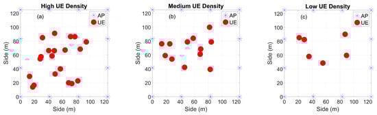
Figure 1. AP and UE positions in a high (a) medium (b) and low (c) UE density RS network.

In Figure 2, Figure 3 and Figure 4 the max–min fairness, max–sum rate and bi-objective power optimization are performed in a high, medium and low UE density RS network with high and low maximum power, respectively. The SE values in both axis are obtained by taking the mean value for the $N_a$ realizations. The $95\%$ confidence intervals are presented. Along with the main SE results, a tendency curve is presented to illustrate an approximation of the non-dominated front. This curve is plotted through a quartic (4th degree) polynomial fitting function.

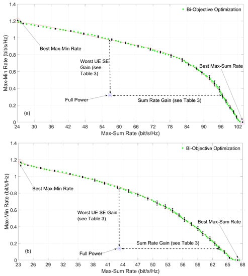
Figure 2. Bi-objective power optimization, max–min fairness and max–sum rate OF in a high UE density RS network with (a) high and (b) low maximum power.

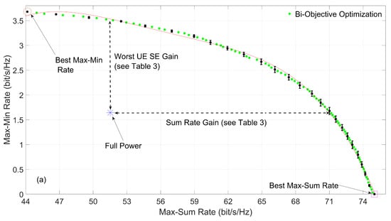
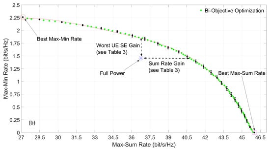
Figure 3. Bi-objective power optimization, max–min fairness and max–sum rate OF in a medium UE density RS network with (a) high and (b) low maximum power.

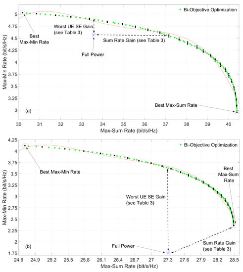
Figure 4. Bi-objective power optimization, max–min fairness and max–sum rate OF in a low UE density RS network with (a) high and (b) low maximum power.

Figure 2a shows the advantage of using an MO approach to unveil the trade-offs between the OFs. The max–min fairness optimization leads to a solution in which the network operates in a state where the worst UE has $1.21$ bit/s/Hz. However, this is achieved at the expense of the sum rate, which is $24.2$ bit/s/Hz for this solution. At the other end, the max–sum rate optimization achieves a total UL throughput of 104 bit/s/Hz, but the worst UE has $2.67\times {10}^{-7}$ bit/s/Hz of SE. The MO optimization approach enables unveiling SE trade-offs between these two extreme operation points. Figure 2a presents all $N_{arch}$ states of network operation computed using the MO version of the DE developed. For reference, it is also displayed the case where there is no power optimization, which means that all UE employ the maximum power, $P_{max}$, (which in this case is 50 mW) in the UL. For this case, the worst UE has a SE of $0.318$ bit/s/Hz, while the network sum rate is $56.8$ bit/s/Hz. In the non-dominated front, we can obtain a point with the same SE for the worst UE, but with a total sum rate of approximately $96.7$ bit/s/Hz, and the same sum rate of $56.8$ bit/s/Hz, with the worst UE having a SE of approximately $0.976$ bit/s/Hz. In these cases, there is a $70.2\%$ gain in the sum rate and a $207\%$ gain in the max–min fairness, respectively, if the network is optimized using the bi-objective approach.

In Figure 2b the max–min fairness optimization has a SE of $1.17$ bit/s/Hz for the worst UE and a sum rate of $23.5$ bit/s/Hz, while the max–sum rate optimization achieves a total of 67 bit/s/Hz with the worst UE having $3.09\times {10}^{-7}$ bit/s/Hz. The point with no power optimization, with $P_{max}=5$ mW, has $0.139$ bit/s/Hz for the worst UE and a sum rate of $43.2$ bit/s/Hz. The bi-objective approach obtains the same SE for the worst UE with a sum rate of approximately $63.7$ bit/s/Hz and the same sum rate with the worst UE having a SE of approximately $0.875$ bit/s/Hz. This represents a $47.5\%$ gain in the sum rate and a $529\%$ gain in the max–min fairness, respectively.

The same trade-offs are observable in Figure 3a where the max–min fairness optimization provides the worst UE with $3.68$ bit/s/Hz but a poor sum rate of $44.1$ bit/s/Hz, while the max–sum rate optimization achieves a total of 75 bit/s/Hz with the worst UE having $3.58\times {10}^{-7}$ bit/s/Hz of SE. For reference, the point with no power optimization for $P_{max}$ = 50 mW is able to obtain $1.64$ bit/s/Hz for the worst UE and $51.5$ bit/s/Hz of network throughput. The MO approach can obtain the same SE for the worst UE with approximately 71 bit/s/Hz of sum rate, and the same throughput with the worst UE having a SE of approximately $3.53$ bit/s/Hz. In both cases, there is a $37.9\%$ gain in the sum rate and a $115\%$ gain in the max–min fairness, respectively.

In Figure 3b the max–min fairness outputs $2.26$ bit/s/Hz for the worst UE and a sum rate of $27.1$ bit/s/Hz, while the max–sum rate outputs 46 bit/s/Hz, with the worst UE having $4.14\times {10}^{-7}$ bit/s/Hz. The point with full power, with $P_{max}=5$ mW, outputs $1.46$ bit/s/Hz for the worst UE and a sum rate of $36.8$ bit/s/Hz. With the MO approach, the same SE for the worst UE is obtained with a sum rate of approximately $40.9$ bit/s/Hz, and the same sum rate is obtained with the worst UE having a SE of approximately $1.84$ bit/s/Hz. The gains are $11.1\%$ and $26\%$ for the max–sum rate and the max–min fairness, respectively.

Figure 4a displays the max–min fairness optimization providing $5.03$ bit/s/Hz for the worst UE with a total sum rate of $30.2$ bit/s/Hz, while the max–sum rate optimization achieves a total of $40.4$ bit/s/Hz, with the worst UE having $2.96$ bit/s/Hz. In this case, by transmitting with full power, with $P_{max}$ = 50 mW, a SE of $4.57$ bit/s/Hz is obtained for the worst UE and the network has a total of $33.6$ bit/s/Hz. The bi-objective approach for the same SE of the worst UE increments the sum rate to approximately 37 bit/s/Hz and for the same throughput increments the SE of the worst UE to approximately $4.89$ bit/s/Hz, thus obtaining gains of about $10.1\%$ and $7\%$ in the sum rate and max–min fairness, respectively.

Finally, Figure 4b shows that it is possible to obtain the extreme points with $4.12$ bit/s/Hz for the worst UE and $24.7$ bit/s/Hz sum rate for the max–min fairness optimization and $28.5$ bit/s/Hz for sum rate combined with $2.36$ bit/s/Hz for the worst UE for the max–sum rate optimization. When transmitting with full power, with $P_{max}$ = 5 mW, the worst UE obtains $1.76$ bit/s/Hz and the network is capable of supporting $27.3$ bit/s/Hz. However, this operation point can be optimized in terms of fairness, where for the same total throughput the worst UE is able to transmit with $3.62$ bit/s/Hz, denoting a gain of about $106\%$. It should be noted that all operation points obtained with the bi-objective optimization approach allows for the worst UE to transmit with SE $\ge 2.36$ bit/s/Hz, which means gains $\ge 34.1\%$ in terms of max–min fairness.

Table 3 summarizes this discussion, where the points of the bi-objective rows are presented with respect to the full power point.

Table 3. SEs obtained through the optimization procedures in bit/s/Hz and the respective gains in %.

		No	Single-Objective		Bi-Objective
		Optimization	Optimization		Optimization
		Full Power	Max–Min	Max–Sum	Sum Rate Gain	Worst UE SE Gain
		(${\mathit{P}}_{\mathbf{max}}$)	Fairness	Rate	Keeping Worst UE SE	Keeping Sum Rate
Scenario 1 High $P_{max}$	Worst UE SE	$0.318$	$1.21$	$2.67\times {10}^{-7}$	$70.2\%$	$207\%$
	Sum Rate	$56.8$	$24.2$	104
Scenario 1 Low $P_{max}$	Worst UE SE	$0.139$	$1.17$	$3.09\times {10}^{-7}$	$47.5\%$	$529\%$
	Sum Rate	$43.2$	$23.5$	67
Scenario 2 High $P_{max}$	Worst UE SE	$1.64$	$3.68$	$3.58\times {10}^{-7}$	$37.9\%$	$115\%$
	Sum Rate	$51.5$	$44.1$	75
Scenario 2 Low $P_{max}$	Worst UE SE	$1.46$	$2.26$	$4.14\times {10}^{-7}$	$11.1\%$	$26\%$
	Sum Rate	$36.8$	$27.1$	46
Scenario 3 High $P_{max}$	Worst UE SE	$4.57$	$5.03$	$2.96$	$10.1\%$	$7\%$
	Sum Rate	$33.6$	$30.2$	$40.4$
Scenario 3 Low $P_{max}$	Worst UE SE	$1.76$	$4.12$	$2.36$	$106\%$	$\ge 34.1\%$
	Sum Rate	$27.3$	$24.7$	$28.5$

5. Conclusions

In this work, an MO MH approach based on the DE algorithm is developed to perform a UL UE power optimization in an RS network. The optimization problem is defined by two metrics to be maximized, the minimum SE of the UE with the worst channel conditions, max–min fairness, and the overall network throughput, max–sum rate. The bi-objective approach is able to provide balanced solutions unveiling relevant trade-offs between the SE performances to assist design decision-making.

References

- Rusek, F.; Persson, D.; Lau, B.K.; Larsson, E.G.; Marzetta, T.L.; Edfors, O.; Tufvesson, F. Scaling Up MIMO: Opportunities and Challenges with Very Large Arrays. IEEE Signal Process. Mag. 2013, 30, 40–60. [Google Scholar] [CrossRef] [Green Version]
- Björnson, E.; Hoydis, J.; Sanguinetti, L. Massive MIMO Networks: Spectral, Energy, and Hardware Efficiency. In Foundations and Trends in Signal Processing; Now Publishers Inc.: Hanover, MA, USA, 2017; Volume 11, pp. 154–655. [Google Scholar]
- Chen, Z.; Björnson, E. Channel Hardening and Favorable Propagation in Cell-Free Massive MIMO with Stochastic Geometry. IEEE Trans. Commun. 2018, 66, 5205–5219. [Google Scholar] [CrossRef] [Green Version]
- Ngo, H.Q.; Ashikhmin, A.; Yang, H.; Larsson, E.G.; Marzetta, T.L. Cell-Free Massive MIMO Versus Small Cells. IEEE Trans. Wirel. Commun. 2017, 16, 1834–1850. [Google Scholar] [CrossRef] [Green Version]
- Larsson, E.G.; Edfors, O.; Tufvesson, F.; Marzetta, T.L. Massive MIMO for next generation wireless systems. IEEE Commun. Mag. 2014, 52, 186–195. [Google Scholar] [CrossRef] [Green Version]
- Pereira, A.; Rusek, F.; Gomes, M.; Dinis, R. On the Complexity Requirements of a Panel-Based Large Intelligent Surface. In Proceedings of the GLOBECOM 2020-2020 IEEE Global Communications Conference, Taipei, Taiwan, 7–11 December 2020; pp. 1–6. [Google Scholar] [CrossRef]
- Zhang, J.; Chen, S.; Lin, Y.; Zheng, J.; Ai, B.; Hanzo, L. Cell-Free Massive MIMO: A New Next-Generation Paradigm. IEEE Access 2019, 7, 99878–99888. [Google Scholar] [CrossRef]
- Chen, C.M.; Blandino, S.; Gaber, A.; Desset, C.; Bourdoux, A.; Van der Perre, L.; Pollin, S. Distributed Massive MIMO: A Diversity Combining Method for TDD Reciprocity Calibration. In Proceedings of the GLOBECOM 2017-2017 IEEE Global Communications Conference, Singapore, 4–8 December 2017; pp. 1–7. [Google Scholar] [CrossRef]
- Björnson, E.; Sanguinetti, L. Making Cell-Free Massive MIMO Competitive with MMSE Processing and Centralized Implementation. IEEE Trans. Wirel. Commun. 2020, 19, 77–90. [Google Scholar] [CrossRef] [Green Version]
- Shaik, Z.; Björnson, E.; Larsson, E.G. Cell-Free Massive MIMO with Radio Stripes and Sequential Uplink Processing. In Proceedings of the 2020 IEEE International Conference on Communications Workshops (ICC Workshops), Dublin, Ireland, 7–11 June 2020; pp. 1–6. [Google Scholar] [CrossRef]
- Shaik, Z.; Björnson, E.; Larsson, E.G. MMSE-Optimal Sequential Processing for Cell-Free Massive MIMO with Radio Stripes. arXiv 2020, arXiv:abs/2012.13928. [Google Scholar] [CrossRef]
- Interdonato, G.; Björnson, E.; Quoc Ngo, H.; Frenger, P.; Larsson, E.G. Ubiquitous Cell-Free Massive MIMO Communications. EURASIP J. Wirel. Commun. Netw. 2019, 2019, 1–13. [Google Scholar] [CrossRef] [Green Version]
- Björnson, E.; Sanguinetti, L. Cell-Free versus Cellular Massive MIMO: What Processing is Needed for Cell-Free to Win? In Proceedings of the 2019 IEEE 20th International Workshop on Signal Processing Advances in Wireless Communications (SPAWC), Cannes, France, 2–5 July 2019; pp. 1–5. [Google Scholar] [CrossRef]
- Nayebi, E.; Ashikhmin, A.; Marzetta, T.L.; Yang, H.; Rao, B.D. Precoding and Power Optimization in Cell-Free Massive MIMO Systems. IEEE Trans. Wirel. Commun. 2017, 16, 4445–4459. [Google Scholar] [CrossRef]
- Zhao, Y.; Niemegeers, I.G.; Groot, S.H.D. Power Allocation in Cell-Free Massive MIMO: A Deep Learning Method. IEEE Access 2020, 8, 87185–87200. [Google Scholar] [CrossRef]
- Bashar, M.; Cumanan, K.; Burr, A.G.; Debbah, M.; Ngo, H.Q. On the Uplink Max–Min SINR of Cell-Free Massive MIMO Systems. IEEE Trans. Wirel. Commun. 2019, 18, 2021–2036. [Google Scholar] [CrossRef] [Green Version]
- Mai, T.C.; Ngo, H.Q.; Duong, T.Q. Uplink Spectral Efficiency of Cell-free Massive MIMO with Multi-Antenna Users. In Proceedings of the 2019 3rd International Conference on Recent Advances in Signal Processing, Telecommunications & Computing (SigTelCom), Hanoi, Vietnam, 21–22 March 2019; pp. 126–129. [Google Scholar] [CrossRef]
- Bashar, M.; Cumanan, K.; Burr, A.G.; Ngo, H.Q.; Poor, H.V. Mixed Quality of Service in Cell-Free Massive MIMO. IEEE Commun. Lett. 2018, 22, 1494–1497. [Google Scholar] [CrossRef] [Green Version]
- Bashar, M.; Cumanan, K.; Burr, A.G.; Ngo, H.Q.; Larsson, E.G.; Xiao, P. Energy Efficiency of the Cell-Free Massive MIMO Uplink with Optimal Uniform Quantization. IEEE Trans. Green Commun. Netw. 2019, 3, 971–987. [Google Scholar] [CrossRef] [Green Version]
- D’Andrea, C.; Zappone, A.; Buzzi, S.; Debbah, M. Uplink Power Control in Cell-Free Massive MIMO via Deep Learning. In Proceedings of the 2019 IEEE 8th International Workshop on Computational Advances in Multi-Sensor Adaptive Processing (CAMSAP), Le Gosier, Guadeloupe, 15–18 December 2019; pp. 554–558. [Google Scholar] [CrossRef] [Green Version]
- Conceição, F.; Antunes, C.H.; Gomes, M.; Silva, V.; Dinis, R. Max-Min Fairness Optimization in Uplink Cell-Free Massive MIMO using Meta-Heuristics. IEEE Trans. Commun. 2022. [Google Scholar] [CrossRef]
- Storn, R.; Price, K. A Simple and Efficient Heuristic for global Optimization over Continuous Spaces. J. Glob. Optim. 1997, 11, 341–359. [Google Scholar] [CrossRef]
- Antunes, C.H.; Alves, M.J.; Clímaco, J. Multiobjective Linear and Integer Programming; Springer: Berlin, Germany, 2016. [Google Scholar]
- Deb, K.; Pratap, A.; Agarwal, S.; Meyarivan, T. A fast and elitist multiobjective genetic algorithm: NSGA-II. IEEE Trans. Evol. Comput. 2002, 6, 182–197. [Google Scholar] [CrossRef] [Green Version]
- Further Advancements for E-UTRA Physical Layer Aspects (Release 9); 3GPP TS 36.814; ETSI: Sophia Antipolis, France, 2010.
Publisher’s Note: MDPI stays neutral with regard to jurisdictional claims in published maps and institutional affiliations. |
© 2022 by the authors. Licensee MDPI, Basel, Switzerland. This article is an open access article distributed under the terms and conditions of the Creative Commons Attribution (CC BY) license (https://creativecommons.org/licenses/by/4.0/).