Abstract
In this paper, we design a joint source and channel coding (JSCC) framework combining the source polar coding and the channel polar coding. The source is first compressed using a polar code (PC), and source check decoding is employed to construct an error set containing the index of all source decoding errors. Then, the proposed JSCC system employs another PC or systematic PC (SPC) to protect the compressed source and the error set against noise, which is called double PC (D-PC) or systematic double PC (SD-PC), respectively. For a D-PC JSCC system, we prove a necessary condition for the optimal mapping between the source PC and the channel PC. On the receiver side, by introducing the joint factor graph representation of the D-PC and SD-PC, we propose two joint source and channel decoders: a joint belief propagation (J-BP) decoder, and a systematic joint belief propagation (SJ-BP) decoder. In addition, a biased extrinsic information transfer (B-EXIT) chart is developed for various decoders as a theoretical performance evaluation tool. Both B-EXIT and simulation results show that the performance of the proposed JSCC scheme has no error floor and outperforms the turbo-like BP decoder.
1. Introduction
The source-channel coding theorem [1] states that a source can be reliably transmitted over a channel as long as its entropy is less than the channel capacity, assuming that latency, complexity, and block length are not constrained. This theorem suggests that we can design source and channel coding separately to achieve optimal results. However, in practical implementations, separate source and channel coding (SSCC) is suboptimal due to the residual redundancy and finite block length. As a potential remedy, joint source and channel coding (JSCC) have been proposed to provide improvements by exploiting residual redundancy and avoiding capacity loss, which can at most double the error exponent vis-a-vis tandem coding [2]. A theoretical study of finite-blocklength bounds for the best achievable lossy JSCC rate demonstrates that JSCC designs bring considerable performance advantages over SSCC in the nonasymptotic regime [3].
One of the main methods of JSCC is the joint decoding of a given source compression format (e.g., JPEG) with a channel decoder. For example, rate-compatible low-density parity-check (RC-LDPC) codes can provide unequal error protection for JPEG2000 compressed images [4]. If the JPEG2000 performs source coding with certain error-resilience (ER) modes, the source decoder can use the ER mode to identify corrupt sections of the codestream for the channel decoder [5]. Iterative decoding of variable-length codes (VLCs) in tandem with channel code can provide remarkable error correction performance [6]. The low-density parity-check (LDPC) codes can be combined with Huffman coded sources to exploit the a priori bit-source probability [7].
Another type of JSCC approach is to assume a Markov model of the source to decode jointly with the factor graph of the channel coding. Joint source-channel Turbo coding for binary Markov sources was investigated in [8]. The drawback of such methods is that the standard VLCs are not suitable for forming a single graph model structure with channel codes (e.g., LDPC codes), as they require long sequences to achieve the entropy of the source. Therefore, a double LDPC (D-LDPC) code for JSCC has been proposed; one LDPC code is used to compress the source first, followed by another LDPC code to protect the compressed source against noise [9]. D-LDPC codes can be represented as a single bipartite graph, allowing the belief propagation (BP) algorithm to decode it on the receiver side. Double protograph LDPC (DP-LDPC) codes are a variant of the D-LDPC codes that introduce a P-LDPC code to replace the conventional LDPC code [10]. Optimization of the base matrix of the DP-LDPC codes can effectively improve the performance of the DP-LDPC JSCC system [11,12,13].
Polar codes, proposed by Arıkan, provably achieve the capacity of any symmetric binary-input discrete memoryless channel (B-DMC) with efficient encoding and decoding algorithms [14]. The successive cancellation algorithm (SC) and belief propagation algorithm (BP) [15] are two commonly used decoding approaches. With the aid of list-decoding, polar codes can outperform LDPC codes at short codelength [16,17,18,19]. Arıkan presented the source polarization as a channel polarization complement [20], which is the theoretical basis for applying polar codes to source compression. Polar codes can achieve the rate-distortion bound for a symmetric binary source for lossy source coding [21]. Moreover, polar codes can asymptotically achieve the optimal compression rate for lossless source coding [22]. Meanwhile, polar code is a good candidate to take advantage of the benefits of source redundancy in the JSCC system [23]. The JSCC system using polar codes can significantly improve the decoding performance for language-based sources and distributed sources [24,25]. A quasi-uniform systematic polar code (qu-SPC) is constructed for the JSCC system with side information by introducing an additional bit-swap coding to modify the original polar coding [26,27]. Our previous work proposes a JSCC scheme with double polar codes by combining source polarization and channel polarization, which shows performance improvement under short codelength [28].
Although polar codes have been studied in the fields of channel coding and source coding, there is a lack of systematic research on the framework of JSCC based on polar codes. In our previous work [28], we introduced the basic double polar code structure of cascading source polar code and channel SPC. However, double polar codes have a high error floor under short blocklength, and lack performance analysis tools in the presence of biased sources.
In this paper, we establish a systematic framework for a JSCC with double polar codes and provide a complete theoretical analysis.
The contributions of this paper are summarized as follows:
- Double Polar Coding Framework: Guided by the source polarization and channel polarization, we propose a JSCC framework based on polar codes, composed of the source polar coding and the channel polar coding. First, a group of source bits is transformed into a series of bit polarized sources by source polarization, where the bit polarized sources with higher entropy, namely, high-entropy bits, are regarded as the compressed source, with other parts are treated as redundancies. After the source is polarized, a source check decoding is performed to construct an error set containing the index of all error decisions that occurred in the source decoding. Second, another polar code (PC) or SPC is used to protect the compressed source bits and the bits in the error set against the noise. Moreover, a mapping is inserted between the source polar code and the PC, where the mapping design affects the performance of the JSCC system. Depending on the channel code, the proposed JSCC scheme is called double polar code (D-PC) or systematic D-PC (SD-PC), respectively. The proposed JSCC framework facilitates the exploitation of residual redundancy in the source code on the decoder side.
- Joint Belief Propagation Decoding: To represent the D-PC and SD-PC, we introduce two factor graphs: the joint factor graph (J-FG) and the systematic joint factor graph (SJ-FG). Correspondingly, the proposed joint source and channel decoder can be divided into two types: the J-TG-based joint belief propagation (J-BP) decoder and the SJ-TG-based systematic joint belief propagation (SJ-BP) decoder. One one hand, for the J-FG, the mapping within D-PC determines the connection between the factor graph of the source code and that of the channel code. The J-BP decoder is iteratively applied over the J-FG, where the source decoder and the source decoder exchange the soft information through the mapping. On the other hand, for the SJ-FG, due to the systematic bits directly carrying high entropy bits, the factor graph of the source code and that of the channel code are combined into a single factor graph. The SD-PC can be decoded as a single factor graph using the SJ-BP decoder.
- B-EXIT Evaluation: Regarding the proposed JSCC system, we present a biased extrinsic information transfer (B-EXIT) convergence analysis for the J-BP decoder and SJ-BP decoder. The EXIT method is extended to consider the non-uniform source. We design a method to calculate the distribution of each high entropy bit, which permits the B-EXIT algorithm to track mutual information transfer for each high entropy bit. This approach reveals the superiority of the proposed JSCC system from a theoretical perspective.
The rest of this paper is organized as follows. Section 2 briefly introduces the background of polar codes and BP decoding. Section 3 proposes the proposed JSCC framework. Section 4 describes the J-BP decoder for D-PC, and Section 5 provides the SJ-BP decoder for SD-PC. Section 6 introduces the B-EXIT chart. Section 7 shows the performance evaluation results with B-EXIT and simulations. Finally, Section 8 concludes the paper.
2. Preliminaries
2.1. Notational Conventions
In this paper, we use calligraphic characters, such as , to denote sets. For any finite set of integers , denotes its cardinality. We denote random variables (RVs) by upper case letters, such as , and their realizations by the corresponding lower case letters, such as . For an RV X, denotes the probability assignment on X. We use the notation as shorthand for denoting a row vector . We use bold letters (e.g., ) to denote matrices. Given and , we write to denote the subvector .
2.2. Polar Codes
A polar code can be identified by a parameter vector , where is the code length, K is the code dimension and specifies the size of the information set, and is the frozen bits. The frozen bits are known to both the transmitter and the receiver, and are usually set to all zeros. Let denote the codeword of a polar code; then, the encoding process can be expressed as , where constitutes of the information bits and frozen bits , while is called the generation matrix of size N and is the nth Kronecker product of the polarizing kernel . Then, the codeword is transmitted over an AWGN channel. The modulation is binary phase shift keying (BPSK). The signals received at the destination are provided by , where is an i.i.d Gaussian noise sequence and each noise sample has zero mean and variance . Furthermore, the LLR of can be written as .
2.3. BP Decoding
An polar code can be represented by an n-stage factor graph which contains nodes. Each -index node is associated with the left-to-right and right-to-right likelihood messages. Let and denote the logarithmic likelihood ratio (LLR)-based left-to-right message and right-to-left message in the t-th iteration. The BP decoder iteratively updates and propagates these soft messages between neighboring nodes over the factor graph. Before decoding starts, is initialized to 0 for ; otherwise, , and is initialized to the channel receive value. The soft messages in the rest of the nodes are initialized to 0. Then, the BP decoder updates the soft message of each node over the whole factor graph. The BP decoder terminates when the number of iterations reaches the preset maximum number of iterations. After the iteration finishes, the estimation of information bits can be obtained by , where the hard-decision function when , and is otherwise 0.
3. Joint Source and Channel Coding
In this section, we present details of the proposed JSCC framework based on the polar code. First, we provide a brief description of the proposed JSCC framework. Then, the coding process of the D-PC scheme and the SD-PC scheme is elaborated.
3.1. Joint Source and Channel Coding Framework
As shown in Figure 1, the proposed JSCC framework mainly comprises two phases: the source polar coding and the channel polar coding. The source polar coding phase involves the source polarization and the check decoding. The source vector is first transformed into a polarized source vector by source polarization. Then, the polarized source vector , which is composed of the high-entropy vector and the low-entropy vector , is fed into a source polar decoder for check decoding. The check decoding generates an error set by collecting the indices of the source decoding errors produced during source decoding. This error set is converted into a binary sequence and appended to the high-entropy vector to form the vector .
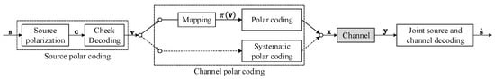
Figure 1.
The JSCC framework based on the polar code.
In the channel polar coding phase, there are two alternative schemes. Let represent a mapping function; for the D-PC scheme, the vector is first mapped to the vector , which is then protected against noise by a PC. For the SD-PC scheme, we directly adopt an SPC to protect the vector . From an overall perspective, in the transmitter, the source vector is coded into the codeword and then transmitted to the receiver through a channel. In the receiver, the received signal is decoded by a joint source and channel decoder to obtain the source estimation .
3.2. Joint Source and Channel Coding for D-PC
The D-PC scheme in the proposed JSCC framework can be implemented by the three procedures described below.
3.2.1. Source Polar Coding
First, the source vector is compressed using a PC. This paper considers an independent and identically distributed (i.i.d.) binary Bernoulli source S with . The source bits from S are represented by the vector . The source polarization of the source vector is performed as follows:
where is the m-order Kronecker power of . Let denote the high-entropy set with . The high-entropy vector are designated as . To avoid errors in recovering at the receiver, we perform a source check decoding to find all indices for which the decision of the corresponding compressed source bit would be incorrect. Let denote the estimation of . Then, a set of indices can be defined as
The final output of the source polar encoding is provided by . Because the size of is at most , each element in can be represented by an m-bit binary sequence. Let denote the binary vector in which all elements of are cascaded in binary form and let . The length of binary vector is denoted as .
The construction of the set has been introduced in [22] based on the SC decoding algorithm. Here, we consider the construction of based on the BP decoding algorithm. In a BP decoder, the estimation is updated in each iteration. Let denote the estimation of in the t-th iteration and let T denote a preset positive integer. If satisfies the convergence condition
we can assume that the converged bit [29]. For , if the converged bit is not equal to , then the index of belongs to . However, if keeps changing without converging, i.e., it remains oscillating, the source BP decoder cannot obtain the converged . To tackle this issue, we propose an oscillation check criterion that considers the corresponding to the maximum LLR amplitude recorded during the oscillation as the converged . Let denote the LLR corresponding to the estimation and let represent with maximum during the oscillation. Moreover, the variable counts the iteration number of the oscillation and is the preset maximum number of oscillations. When , the can be provided by
where when and is otherwise , then the set includes the index i if .
3.2.2. Optimal Mapping
For the D-PC JSCC system, the polarized sub-channels with the highest capacity carry the vector , where the high-entropy vector consists of polarized source bits. Because the block length is finite, the polarization of both the source and the channel is insufficient. When one polarized source bit is transmitted over a polarized channel, if the entropy of the former is less than the mutual information of the latter, such transmission is unreliable. Therefore, we need to optimize the mapping between the source and channel codes to improve system performance. From the perspective of mutual information maximization, we provide Theorem 1, which states a necessary condition for the optimal mapping.
Theorem 1.
For a double polar code identified by a parameter vector , there exists an optimal mapping π between the source polar code and channel polar code that maximizes the mutual information . The optimal mapping must satisfy
for all and .
Proof of Theorem 1.
Consider a mapping . In the coding process, the high-entropy bits are carried by the information bits ; then, there is with in the decoding process. The mutual information is calculated as follows:
The information bit is transmitted over the polarized channel . The mutual information is not able to exceed the channel capacity . The vector is transmitted over polarized channels . Let denote the j-th element of the set . Based on the chain rule for entropy, we have
If the index corresponds to the j-th element of the set , the can be rewritten as
As a result of , we can obtain
Thus, we have the following relationships:
Then, we can obtain the following inequality:
The compressed bit is assigned to by the mapping. Accordingly, (11) can be rewritten as follows:
Based on Theorem 1, we propose Algorithm 1 to construct an optimal mapping. Let and denote the ith element of and . We use a sequence to denote the sorted by the descending order of reliability. Moreover, a sequence is used to denote the sorted by descending order of entropy. Let a sequence denote the mapping , where indicates that is mapped to , i.e., is transmitted by the sub-channel . In Algorithm 1, the most reliable polarized sub-channel transmits the polarized source bit with the highest entropy. Meanwhile, the least reliable polarized sub-channel transmits the polarized source bit with the lowest entropy.
| Algorithm 1:Construct the mapping . |
 |
3.2.3. Channel Polar Coding
Finally, we protect the compressed source bits and the bits in the error set with another PC. Let denote the information set of the channel PC with . The encoding of the PC has been described in Section 2.2. We can write the encoding process as
Because , (13) can be rewritten as
3.3. Joint Source and Channel Coding for SD-PC
The difference between SD-PC and D-PC is that SD-PC employs an SPC to protect the vector . We can split the codeword into two parts by writing , where is the codeword length and the systematic bits are assigned to the vector . For the SPC, the parity bits are provided by
where is an all-zero subvector and denotes the submatrix of consisting of the array of elements , with and , and submatrix can be similarly defined. Then, is calculated as follows:
In summary, the source polar coding and channel polar coding can form a JSCC framework. For the D-PC JSCC system, the optimal mapping can maximize the mutual information between the compressed source bits and the corresponding estimation .
4. Joint Source and Channel Decoding of D-PC
In this section, we first extend the factor graph representation to the D-PC, namely, J-FG. Second, we propose a joint source and channel decoding algorithm based on the J-FG, i.e., the J-BP decoder.
4.1. Joint Tanner Graph Representation
The polar codes can be represented by a factor graph, which can be generalized to the D-PC; that is to say, the source polar code with code length and the channel polar code with code length can be described by a factor graph with m stages and a graph with n stages, respectively. Therefore, the D-PC can be illustrated by a joint factor graph (J-FG) with stages, where . In the J-FG, the part depicting the source code is called the source factor graph (SFG), and the part that represents the channel code is called the channel factor graph (CFG).
The J-FG of the D-PC is shown in Figure 2. For the D-PC, the high-entropy bits of the source polar code are assigned to the information bits of the channel polar code, which is the basis for constructing the J-FG. The m stages on the left side of the J-FG are the SFG, and the n stages on the right side of the J-FG are the CFG. In this J-FG, the variable nodes in the leftmost column correspond to the source vector and the variable nodes in the rightmost column correspond to the codeword . The channel polar code does not directly carry the vector with the information bits in the D-PC scheme; rather, it carries after mapping. Accordingly, the variable node corresponding to the high-entropy bits in SFG is connected to the variable node corresponding to in CFG through a mapping. The vector contained in can be ignored, as the bits in the vector do not have corresponding variable nodes in the SFG. Thus, we can obtain the J-FG of the D-PC scheme.
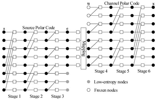
Figure 2.
The joint factor graph of the D-PC scheme.
4.2. Joint Belief Propagation Decoding
The Turbo-like BP (TL-BP) decoder [28] consists of a channel BP decoder and source BP decoder. External information interaction between two independent decoders implements joint decoding in [28]. Unlike TL-BP decoding, the J-BP decoder iteratively operates over the entire J-FG representing the D-PC, and no longer distinguishes between the source BP decoder and the channel BP decoder. A high-level description of the J-BP decoding algorithm is provided in Algorithm 2. The J-FG has stages and columns, which from left to right are the 0th to the th column, respectively. Each node is associated with LLR messages and . These messages are updated and propagated among adjacent nodes during the whole iteration process.
| Algorithm 2:A High-Level Description of the Joint Source and Channel Decoder. |
 |
4.2.1. Initialization
We first initialize the J-BP decoder. This paper considers a binary Bernoulli source S with . Thus, the initialization of can be provided by
As shown in Figure 2, the variable nodes in the rightmost column correspond to the codeword ; hence, for . Furthermore, we know that the frozen bits are ‘0’. Thus, the initialization of the can be described by
The messages in the remaining variable nodes of the J-FG are all initialized to zeros.
4.2.2. Iteration Decoding
After initialization is complete the J-BP decoder is activated, which is carried out on Lines 2–9 of Algorithm 2. The maximum number of iterations of the J-BP decoder is preset and denoted as . One iteration of the J-BP decoder consists of left-to-right and right-to-left message propagation. In the left-to-right message propagation, the J-BP decoder updates serially in the order of . Then, the J-BP decoder updates from right to left in the order . The message update rule employed by the J-BP decoder is the same as the conventional BP decoder.
The message update rule of a processing element is described by
where is as follows:
Recall the optimal mapping between the source code and the channel code, as shown in Figure 2; because soft message exchange between SFG and CFG involves the mapping, we describe this in greater detail below.
In the J-BP decoder of the D-PC scheme, soft messages are transferred to CFG through a mapping. In contrast, soft messages are transferred to SFG through an inverse mapping. Let denote the inverse of the mapping . Then, the soft message exchange between SFG and CFG can be expressed by
for and .
To avoid redundant iterations, we apply the early stopping criterion for the J-BP decoder. For the early stopping criterion of the BP decoder for the polar codes, refer to [30]. If the early stopping criterion holds for both the source PC and channel PC, the J-BP decoder terminates and outputs the estimation of the source. The estimation of the source is denoted as , which can be obtained by
Otherwise, the lossless BP decoding is activated if the early stopping criterion holds only for the channel polar code (Lines 7–9, Algorithm 2).
4.2.3. Lossless Source BP Decoding
The description of the lossless source BP decoding is provided in Algorithm 3. The channel polar code can be regarded as having been decoded successfully if the early stopping criterion holds for the channel polar code, which means we can obtain the estimation of . For the J-BP decoder, the estimation can be calculated by
where . The estimation can be divided into two parts, and . Therefore, the SFG of J-BP decoder can be reinitialized based on as follows:
Meanwhile, we can use the vector to recover the error set , which is shown in Line 2 of Algorithm 3. One element of the set is represented by a binary vector of m bits. The cardinality of can be obtained by , i.e., the number of errors that occur in the source BP decoding can be known. If the cardinality of is not zero, we can convert every m bits of the binary vector into a decimal number to obtain an element of . After recovering the error set , the source decoding errors can be corrected, as we already know in advance the indices of errors that will occur during the source decoding process.
| Algorithm 3:Lossless BP Source Decoding. |
 |
The estimation can be updated by executing a BP decoding over SFG. If satisfies the convergence condition (3), it can be assumed that the estimation has converged. However, there exist some that constantly keep changing during iteration; this is called the oscillation error, in which case the convergence condition (3) is invalid. To solve this oscillation error, we take the with the largest absolute value recorded during the oscillation as the converged , which is a recall of (4). If , the converged is regarded as a correct estimation. Furthermore, we can obtain the correct estimation by flipping the converged if . The lossless source BP decoding terminates when the iteration number reaches the preset maximum or the estimation converges. In the end, the source estimation can be obtained by re-encoding .
5. Joint Source and Channel Decoding of SD-PC
In this section, we first extend the factor graph representation to the SD-PC, which we call SJ-FG. Second, we propose a joint source and channel decoding algorithm based on J-FG, i.e., the SJ-BP decoder.
5.1. Systematic Joint Factor Graph Representation
The SD-PC can be represented by an -stages SJ-FG, where . For the SD-PC scheme, the high-entropy bits of the source PC are directly transmitted by the systematic bits of the channel SPC. Therefore, the variable node corresponding to the high-entropy bit can be connected with the variable node corresponding to the systematic bit by a check node. Figure 3 shows an SJ-FG of the SD-PC scheme. In this SJ-FG, the m stages on the left side represent the source PC and the n stages on the right side represent the channel SPC. The check nodes connect the source high-entropy nodes and the channel systematic nodes. The variable nodes in the leftmost column correspond to the source vector , and the variable nodes in the rightmost column correspond to the vector .
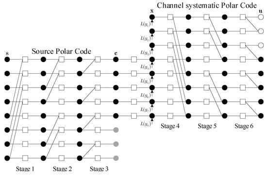
Figure 3.
The systematic joint factor graph of the SD-PC scheme.
5.2. Systematic Joint Source and Channel Decoding
The SJ-BP decoder iteratively operates over the SJ-FG representing the SD-PC. The high-level description of the SJ-BP decoding algorithm has been provided in Algorithm 2. The details of the SJ-BP decoder are presented as follows.
5.2.1. Initialization
The initialization of is provided in (18). For , the message associated with the parity check node is initialized by . The variable nodes corresponding to the frozen bits are located in the rightmost column. The message can be initialized by
Moreover, the messages in the remaining variable nodes in the SJ-FG are all initialized to zeros.
5.2.2. Iteration Decoding
The SJ-BP decoder is activated after initialization is complete. The message passing schedule of the SJ-BP decoder is the same as the J-BP decoder. The message update rule employed by the SJ-BP decoder has been described by (20). The soft message exchange between SFG and CFG can be expressed as follows:
where is the ith element of the set and is the ith element of the set . The SJ-BP decoding is terminated when the source PC and channel SPC satisfy the early stopping criterion or the iteration number reaches the preset maximum, . If the early stopping criterion holds only for the channel SPC, the lossless source BP decoding is activated.
5.2.3. Lossless Source BP Decoding
When the early stopping criterion holds for the channel SPC, the estimation can be calculated by
where . Then, we split the vector into the estimation and , where is further recovered as the set . Because source polar coding is common to the D-PC and SD-PC schemes, the lossless source BP decoding is the same in both the J-BP decoder and the SJ-BP decoder, which has been provided in Algorithm 3.
6. B-EXIT Convergence Analysis
EXIT chat [31] is an efficient tool for analyzing the convergence of the iterative decoder. It provides an excellent visual representation of the iterative decoder by tracking the mutual information (MI) at each iteration. In this section, we perform a biased-EXIT (B-EXIT) convergence analysis for the proposed JSCC system with binary Bernoulli source. To evaluate the convergence performance of the J-BP decoder and the SJ-BP decoder under binary Bernoulli source, we track the average MI (AMI) transfer process between SFG and CFG such that we can provide a virtual representation of the iterative decoding process. The EXIT method is named B-EXIT due to the biased source, which is shown in Algorithm 4.
| Algorithm 4:B-EXIT analysis. |
 |
For a uniform source, it can be assumed without loss of generality that the codeword sent is all zeros, which is not reasonable for a biased source. Therefore, as shown in lines 2–3 of Algorithm 4, we actually generate a codeword for the D-PC or SD-PC with a biased source and record the compressed bits . Then, the receiver obtains the signal by sending the codeword over the binary phase shift keying (BPSK) modulated additive white Gaussian noise (AWGN) channel. Based on the received signal and the source distribution , the joint source-channel decoder, i.e., the J-BP decoder and SJ-BP decoder, can be initialized.
For the t-th iteration of the J-BP decoder, let denote the a priori AMI between the input LLRs and the compressed bits. Similarly, is used to denote the extrinsic AMI between the output LLRs and the compressed bits. For the J-BP decoder and SJ-BP decoder, the input LLRs actually refer to (), which represents the input LLRs of the CFG (SFG). Similarly, the output LLRs refer to (), which represents the output LLRs of the CFG (SFG). To track the decoding trajectory, we collect all the and at each iteration by using a number of simulated code blocks (Line 6, Algorithm 4). For , let to collect when , and let to collect when . In line 7 of Algorithm 4, for we utilize to count the PDFs with the histogram method. The can be utilized to count PDFs with the histogram method.
After the probability density functions (PDFs) of these LLRs have been counted with the histogram method, we can calculate the AMI . The compressed bits are not uniform due to the source being biased. Therefore, we first need to calculate the mutual information between each compressed bit and the corresponding LLR independently. Let denote the mutual information between the compressed bit and ; we can obtain by the histogram method. Here, refers to the probability distribution of compressed bits . The probability distribution of each bit in is different. The compressed bits are obtained by multiplying the source sequence and the ith column of the generation matrix. Let the set denote the index of ‘1’ in the ith column of the generation matrix and let denote the Hamming weight of the ith column of the generation matrix. Then, we have
for . Here, is the probability that the number of ones in the sequence is odd. Thus, we can obtain the distribution of the compressed bits as follows [32]:
where p is of a Bernoulli source S. After obtaining the probability distribution of compressed bits , we can calculate . Then, the AMI is provided by
The computed AMI can be plotted as a zigzag path, which reflects the decoding trajectory. On the EXIT plane, AMI pairs can be written as the coordinate points, which can be expressed as follows:
where . By connecting the vertices at both ends of the zigzag path separately, we can obtain two curves, corresponding to and . We now connect the adjacent coordinate points in the form
where . Then, we obtain the extrinsic AMI transfer trajectory. After obtaining the extrinsic AMI transfer trajectory, the convergence speed of the proposed joint source-channel decoder with finite coding length and limited number of iterations can be reflected.
7. Performance Evaluation
In this section, we illustrate the advantages of the proposed JSCC system. We begin with a binary Bernoulli source S with . Let denote the compression rate and denote the overall rate of the JSCC system. We simulate the bit error rate (BER) performance of the proposed JSCC system over the binary phase shift keying (BPSK) modulated additive white Gaussian noise (AWGN) channel. For all these results, the signal-to-noise ratio is represented by , where refers to the energy per source bit and denotes the noise power. The employed polar code is constructed by the Gaussian approximation method [33].
7.1. B-EXIT Analysis
The B-EXIT analysis of the proposed JSCC system for a binary Bernoulli source with is provided in this part. Two EXIT charts are shown in Figure 4, where the iteration number is . In Figure 4a with dB, we can observe that the extrinsic AMI increment step of the J-BP decoder sees an improvement if the optimal mapping is introduced in the D-PC. In the region with , the convergence of J-BP is faster than that of J-BP (no ), where “no ” means that the optimal mapper is removed in the D-PC scheme. When is larger than 0.8, the decoding trajectories of J-BP and J-BP (no ) gradually approach each other. Figure 4b shows that the extrinsic AMI increment step of the SD-PC is superior to the D-PC with dB. In the region where is less than 0.6, the SJ-BP decoder converges significantly faster than the J-BP decoder. The convergence of the J-BP decoder is accelerated when is greater than 0.6, although the final convergence coordinate of the J-BP decoder remains significantly lower than that of the SJ-BP decoder.
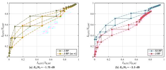
Figure 4.
Two B-EXIT charts with iterations: (a) impact of the optimal mapping for the D-PC scheme with dB and (b) performance comparison between D-PC and SD-PC with dB.
7.2. Simulation Results
The BER results of the J-BP decoder and the SJ-BP decoder are provided in Figure 5 with , , and the overall rate . The source compression rate is chosen from . For comparison, the BER curves of the TL-BP decoder [28] are provided as benchmarks in Figure 5a. For a fair comparison with the TL-BP decoder, we set the maximum number . Meanwhile, to reduce complexity, the G-Matrix [30] and cyclic redundancy check-aided (CA) [34] early stopping criterion are applied to the source polar code and the channel polar code, respectively.
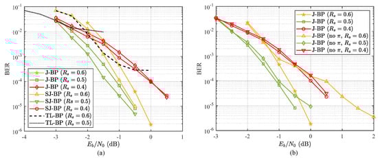
Figure 5.
BER performance comparison: (a) J-BP decoding, SJ-BP decoding and TL-BP decoding; (b) J-BP decoding vs J-BP (no ) decoding [28].
In Figure 5a, we observe that the J-BP decoder shows no significant error floor compared with the TL-BP decoder [28]. The error floor of the TL-BP decoder is at the level with the compression rate . Moreover, the error floor of the TL-BP decoder deteriorates further to the level as the compression rate is set to 0.5. As a comparison, the error floor does not appear in the performance curve of the J-BP decoder or the SJ-BP decoder. The proposed JSCC system transmits the index of the error decision that occurs in the source decoding along with the compressed source through the channel. Therefore, as long as the channel decoding is correct we can know the index of the error decision and correct the source decoding, which is the reason for the disappearance of the error floor.
In addition, Figure 5a shows that the SJ-BP decoder outperforms the J-BP decoder. For and , the SJ-BP decoder compared to the J-BP decoder yields 0.30 dB and 0.28 dB gain at , respectively. For SD-PC, the SJ-BP decoder can obtain 0.41 dB gain when is reduced from 0.6 to 0.5 at . With a constant overall rate R, the lower compression rate implies a lower channel coding rate , which is the reason for the additional gain. However, if is further reduced to 0.4, the performance of the J-BP decoder deteriorates instead. The lower leads to an increase in source decoding errors, and therefore the actual compression rate rises due to the need to transmit a larger error set . In Table 1, we provide the average actual compression rate of the proposed JSCC system with various p. It can be observed that the actual compression rate increases only slightly for and , while for the actual compression rate rises to 0.4559. The excessive rise in the average actual compression rate causes a significant loss in the performance of the JSCC system. In Figure 5a, a slight performance loss can be observed in the low region for the SJ-BP decoder compared to the TL-BP decoder, as the actual compression rate is slightly larger than the preset compression rate . For , the J-BP decoder has 0.18 dB performance loss compared with the TL-BP decoder at , which is due to the superior BER performance of SPC over PC [27]. Figure 5b demonstrates the effect of the optimal mapping for the D-PC scheme. In the lower region, the effect of the optimal mapping on the performance of the D-PC scheme is not obvious. The gain from the optimal mapping rises with the . When and , the optimal mapping brings a gain of 1.67 dB and 0.51 dB, respectively, to the D-PC scheme at . Removing the optimal mapping from the D-PC scheme causes significant performance loss in the high region. For , the optimal mapping reduces the gain to 0.16 dB at , which is again due to an excessive increase in the actual compression rate.

Table 1.
Actual compression rate of the source polar coding.
Figure 6 provides a comparison of the SD-PC employing SPC with the DP-LDPC codes. To facilitate the comparison with the last DP-LDPC [13], the source code and the channel code with half the rate are designed. The overall rate of the JSCC system is 1. From Figure 6, it can be observed that the SD-PC achieves significant performance gains in the high region due to the absence of an error floor. For the source block length with , the SD-PC has a 0.7 dB performance gap compared to DP-LDPC at . As p decreases to 0.04, the performance gap reaches 0.9 dB. The DP-LDPC codes perform better than the D-Polar codes at low . However, we can observe that the DP-LDPC codes suffer from a severe error floor at short code length, which is a weakness that the SD-PC does not have. Because the SD-PC is not subject to an error floor, we can further reduce the compression rate to obtain greater gain without causing an increase in the error. As shown in Figure 6, the performance of the SD-PC in the low region is close to that of DP-LDPC codes when , at which point the performance gap is reduced to 0.1 dB. Reducing to obtain the decoding gain of the JSCC system is not suitable for DP-LDPC codes due to their already high error floor.
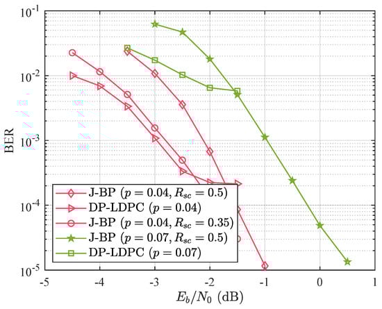
Figure 6.
BER performance of the SD-PC JSCC system versus the DP-LPDC JSCC system with [13].
7.3. Complexity Analysis
For both the D-PC and SD-PC, the coding complexity is and the joint source-channel decoding involves source decoding and channel decoding. Let I denote the iteration number; the complexity of the J-BP decoding and SJ-BP decoding is . When the number of iterations is high, the high complexity of the decoding limits the application of the double polar codes. Figure 7 shows the average iteration number of the J-BP decoder and the SJ-BP decoder. The SJ-BP decoder has the lowest average iteration number. In Figure 7, all curves fall rapidly as increases. Overall, the curve of the average iteration number shifts left as the compression rate decreases from to . However, for the number of iterations increases as the compression rate decreases, which is due to the same reasons as the performance loss presented in Section 7.2. For the D-PC, the presence of the optimal mapping leads to an increase in the iteration number in the low region and a decrease in the iteration number in the high region. The optimal mapping provides an advantage in reducing the decoder complexity in the low region.
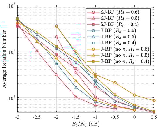
Figure 7.
Average iteration number of J-BP decoder with .
8. Conclusions
In this paper, a JSCC framework has been proposed which combines source polar coding and channel polar coding. The source is first compressed by a PC, then protected by another PC or SPC. To avoid the error floor, the source polar coding employs a source check decoding to construct the error set, collecting the index of source decoding error. The construction and transmission of the error set ensures that the source decoding definitely succeeds as long as the channel decoding is correct. For the D-PC JSCC system, we prove a necessary condition of the optimal mapping to maximize the MI between the compressed source bits and its estimation. The D-PC and SD-PC can be represented by the J-FG and SJ-FG. On the receiver side, the J-BP decoder and SJ-BP decoder are proposed based on the J-FG and SJ-FG. By calculating the probability distribution of the compressed bits, B-EXIT is developed to analyze the decoding trajectory of the proposed joint source-channel decoder with a binary Bernoulli source. The simulation results show that the proposed JSCC system does not suffer from an error floor. Moreover, theoretical analysis and simulation results show that the SD-PC scheme is optimal, while the optimal mapping can improve the performance of the D-PC scheme. Note that we only consider AWGN channels in this paper. The optimal design of double polar codes in fading channels remains an open problem.
Author Contributions
This work was mainly performed by Y.D. (planning of the work, conceptualisation, investigation, methodology, data curation, resources, software, visualisation, and original draft preparation) and was completed with key contributions from K.N. (planning of the work, conceptualisation, supervision, manuscript review and editing, and funding acquisition). All authors have read and agreed to the published version of the manuscript.
Funding
This research was supported in part by the National Natural Science Foundation of China under Grant 92067202, Grant 62071058, Grant 62001049.
Conflicts of Interest
The authors declare no conflict of interest.
References
- Shannon, C.E. A mathematical theory of communication. Bell Syst. Tech. J. 1948, 27, 379–423. [Google Scholar] [CrossRef]
- Zhong, Y.; Alajaji, F.; Campbell, L. On the joint source-channel coding error exponent for discrete memoryless systems. IEEE Trans. Inf. Theory 2006, 52, 1450–1468. [Google Scholar] [CrossRef]
- Kostina, V.; Verdu, S. Lossy Joint Source-Channel Coding in the Finite Blocklength Regime. IEEE Trans. Inf. Theory 2013, 59, 2545–2575. [Google Scholar] [CrossRef]
- Pan, X.; Cuhadar, A.; Banihashemi, A. Combined source and channel coding with JPEG2000 and rate-compatible low-density Parity-check codes. IEEE Trans. Signal Process. 2006, 54, 1160–1164. [Google Scholar] [CrossRef]
- Pu, L.; Wu, Z.; Bilgin, A.; Marcellin, M.W.; Vasic, B. LDPC-Based Iterative Joint Source-Channel Decoding for JPEG2000. IEEE Trans. Image Process. 2007, 16, 577–581. [Google Scholar] [CrossRef]
- Zribi, A.; Pyndiah, R.; Zaibi, S.; Guilloud, F.; Bouallegue, A. Low-Complexity Soft Decoding of Huffman Codes and Iterative Joint Source Channel Decoding. IEEE Trans. Commun. 2012, 60, 1669–1679. [Google Scholar] [CrossRef]
- Mei, Z.; Wu, L. Joint Source-Channel Decoding of Huffman codes with LDPC codes. J. Electron. 2006, 23, 806–809. [Google Scholar] [CrossRef]
- Zhu, G.C.; Alajaji, F. Joint source-channel turbo coding for binary Markov sources. IEEE Trans. Wirel. Commun. 2006, 5, 1065–1075. [Google Scholar] [CrossRef]
- Fresia, M.; Perez-Cruz, F.; Poor, H.V.; Verdu, S. Joint Source and Channel Coding. IEEE Signal Process. Mag. 2010, 27, 104–113. [Google Scholar] [CrossRef]
- He, J.; Wang, L.; Chen, P. A joint source and channel coding scheme base on simple protograph structured codes. In Proceedings of the 2012 International Symposium on Communications and Information Technologies (ISCIT), Gold Coast, Australia, 2–5 October 2012; pp. 65–69. [Google Scholar] [CrossRef]
- Chen, C.; Wang, L.; Lau, F.C.M. Joint Optimization of Protograph LDPC Code Pair for Joint Source and Channel Coding. IEEE Trans. Commun. 2018, 66, 3255–3267. [Google Scholar] [CrossRef]
- Chen, Q.; Wang, L.; Hong, S.; Chen, Y. Integrated Design of JSCC Scheme Based on Double Protograph LDPC Codes System. IEEE Commun. Lett. 2019, 23, 218–221. [Google Scholar] [CrossRef]
- Liu, S.; Wang, L.; Chen, J.; Hong, S. Joint Component Design for the JSCC System Based on DP-LDPC Codes. IEEE Trans. Commun. 2020, 68, 5808–5818. [Google Scholar] [CrossRef]
- Arıkan, E. Channel Polarization: A Method for Constructing Capacity-Achieving Codes for Symmetric Binary-Input Memoryless Channels. IEEE Trans. Inf. Theory 2009, 55, 3051–3073. [Google Scholar] [CrossRef]
- Arikan, E. A performance comparison of polar codes and Reed-Muller codes. IEEE Commun. Lett. 2008, 12, 447–449. [Google Scholar] [CrossRef]
- Niu, K.; Chen, K. CRC-Aided Decoding of Polar Codes. IEEE Commun. Lett. 2012, 16, 1668–1671. [Google Scholar] [CrossRef]
- Chen, K.; Niu, K.; Lin, J. Improved Successive Cancellation Decoding of Polar Codes. IEEE Trans. Commun. 2013, 61, 3100–3107. [Google Scholar] [CrossRef]
- Niu, K.; Chen, K.; Lin, J.; Zhang, Q.T. Polar codes: Primary concepts and practical decoding algorithms. IEEE Commun. Mag. 2014, 52, 192–203. [Google Scholar] [CrossRef]
- Tal, I.; Vardy, A. List Decoding of Polar Codes. IEEE Trans. Inf. Theory 2015, 61, 2213–2226. [Google Scholar] [CrossRef]
- Arıkan, E. Source polarization. In Proceedings of the 2010 IEEE International Symposium on Information Theory, Austin, TX, USA, 13–18 June 2010; pp. 899–903. [Google Scholar]
- Korada, S.B.; Urbanke, R. Polar codes are optimal for lossy source coding. In Proceedings of the 2009 IEEE Information Theory Workshop, Volos, Greece, 10–13 June 2009; pp. 149–153. [Google Scholar]
- Cronie, H.S.; Korada, S.B. Lossless source coding with polar codes. In Proceedings of the 2010 IEEE International Symposium on Information Theory, Austin, TX, USA, 13–18 June 2010; pp. 904–908. [Google Scholar] [CrossRef]
- Wang, Y.; Narayanan, K.R.; Jiang, A.A. Exploiting source redundancy to improve the rate of polar codes. In Proceedings of the 2017 IEEE International Symposium on Information Theory (ISIT), Aachen, Germany, 25–30 June 2017; pp. 864–868. [Google Scholar] [CrossRef]
- Wang, Y.; Qin, M.; Narayanan, K.R.; Jiang, A.; Bandic, Z. Joint Source-Channel Decoding of Polar Codes for Language-Based Sources. In Proceedings of the 2016 IEEE Global Communications Conference (GLOBECOM), Washington, DC, USA, 4–8 December 2016; pp. 1–6. [Google Scholar]
- Jin, L.; Yang, P.; Yang, H. Distributed Joint Source-Channel Decoding Using Systematic Polar Codes. IEEE Commun. Lett. 2018, 22, 49–52. [Google Scholar] [CrossRef]
- Jin, L.; Yang, H. Joint Source-Channel Polarization With Side Information. IEEE Access 2018, 6, 7340–7349. [Google Scholar] [CrossRef]
- Arikan, E. Systematic Polar Coding. IEEE Commun. Lett. 2011, 15, 860–862. [Google Scholar] [CrossRef]
- Dong, Y.; Niu, K.; Dai, J.; Wang, S.; Yuan, Y. Joint Source and Channel Coding Using Double Polar Codes. IEEE Commun. Lett. 2021, 25, 2810–2814. [Google Scholar] [CrossRef]
- Simsek, C.; Turk, K. Simplified Early Stopping Criterion for Belief-Propagation Polar Code Decoders. IEEE Commun. Lett. 2016, 20, 1515–1518. [Google Scholar] [CrossRef]
- Yuan, B.; Parhi, K.K. Early Stopping Criteria for Energy-Efficient Low-Latency Belief-Propagation Polar Code Decoders. IEEE Trans. Signal Process. 2014, 62, 6496–6506. [Google Scholar] [CrossRef]
- Ten Brink, S. Convergence behavior of iteratively decoded parallel concatenated codes. IEEE Trans. Commun. 2001, 49, 1727–1737. [Google Scholar] [CrossRef]
- Gallager, R. Low-density parity-check codes. IRE Trans. Inf. Theory 1962, 8, 21–28. [Google Scholar] [CrossRef]
- Trifonov, P. Efficient Design and Decoding of Polar Codes. IEEE Trans. Commun. 2012, 60, 3221–3227. [Google Scholar] [CrossRef]
- Ren, Y.; Zhang, C.; Liu, X.; You, X. Efficient early termination schemes for belief-propagation decoding of polar codes. In Proceedings of the 2015 IEEE 11th International Conference on ASIC (ASICON), Chengdu, China, 3–6 November 2015; pp. 1–4. [Google Scholar] [CrossRef]
Publisher’s Note: MDPI stays neutral with regard to jurisdictional claims in published maps and institutional affiliations. |
© 2022 by the authors. Licensee MDPI, Basel, Switzerland. This article is an open access article distributed under the terms and conditions of the Creative Commons Attribution (CC BY) license (https://creativecommons.org/licenses/by/4.0/).