A Greedy Heuristic Based on Optimizing Battery Consumption and Routing Distance for Transporting Blood Using Unmanned Aerial Vehicles

Abstract

Unmanned Aerial Vehicles (UAVs) play crucial roles in numerous applications, such as healthcare services. For example, UAVs can help in disaster relief and rescue missions, such as by delivering blood samples and medical supplies. In this work, we studied a problem related to the routing of UAVs in a healthcare approach known as the UAV-based Capacitated Vehicle Routing Problem (UCVRP). This is classified as an NP-hard problem. The problem deals with utilizing UAVs to deliver blood to patients in emergency situations while minimizing the number of UAVs and the total routing distance. The UCVRP is a variant of the well-known capacitated vehicle routing problem, with additional constraints that fit the shipment type and the characteristics of the UAV. To solve this problem, we developed a heuristic known as the Greedy Battery—Distance Optimizing Heuristic (GBDOH). The idea was to assign patients to a UAV in such a way as to minimize the battery consumption and the number of UAVs. Then, we rearranged the patients of each UAV in order to minimize the total routing distance. We performed extensive experiments on the proposed GBDOH using instances tested by other methods in the literature. The results reveal that GBDOH demonstrates a more efficient performance with lower computational complexity and provides a better objective value by approximately 27% compared to the best methods used in the literature.

1. Introduction

Natural disasters—such as earthquakes, volcanoes, avalanches, tornadoes, forest fires, and floods—rank among the greatest threats to humanity and the environment. They have a tragic impact on lives, where they leave behind critical injuries and change and affect the terrain. Patients in emergency or post-disaster situations often encounter difficulties obtaining medical help and supplies (especially blood) in a timely manner. Sending blood supplies to injured patients in inaccessible locations can prove indispensable in saving human lives. The greatest challenge in sending blood to patients is the difficulty or impossibility (in most cases) of using land transportation due to post-disaster environmental conditions and transportation infrastructures (e.g., roads might become obstructed, and bridges might be cracked [1]). Moreover, the blood temperature may change during transportation.

To transcend these challenges, it is crucial to design and implement an efficient algorithm to assist patients in emergency or post-disaster situations using transport that is not hampered by transportation infrastructure and is not much more expensive than land transportation. This aim can be accomplished by utilizing Unmanned Aerial Vehicles (UAVs). UAVs have proven suitable in various applications when used in harsh conditions, such as agriculture, transport, aerial photography, and data collection [2]. In addition, UAVs have been utilized in healthcare applications (Figure 1). For example, UAVs were used to deliver medicines and temperature-sensitive COVID-19 vaccines in Malawi [3], Zipline UAVs were used to transport vaccines and blood [4], UAVs were used to track malaria outbreaks in Africa [5], and Shenzhen Smart UAVs were used to spray chemical substances to reduce the prevalence of COVID-19 in China [6].

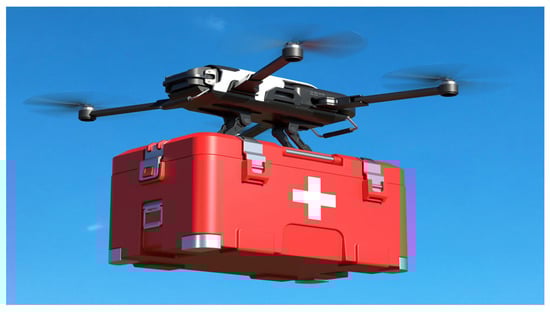
Figure 1. Example of using drones to transport blood. Reprinted with permission from ref. [7]. Copyright 2022 Shutterstock, Inc.

However, healthcare applications require distinct considerations related to their circumstances and how to maximize their services. For example, blood should be delivered to patients quickly while guaranteeing the blood’s viability [8]. In such instances, the compliance of healthcare applications with these considerations proves critical [8,9].

In light of the above points, this study investigates problems in emergency situations that healthcare workers may face—namely, the delivery of viable blood to patients using the smallest number of UAVs and the shortest routing distance [10]. In the literature, this problem is known as the UAV-based Capacitated Vehicle Routing Problem (UCVRP) [10], which is concerned with finding the optimal or a near-optimal solution for the UAV-based Capacitated Vehicle Routing Problem for delivering blood to patients in emergency situations. The UCVRP is a variant of the well-known Capacitated Vehicle Routing Problem (CVRP). The CVRP is a typical NP-hard combinatorial optimization problem [11]. Typically, NP-hard problems are solved by heuristic or metaheuristic algorithms [12,13,14], which can obtain optimal or near-optimal solutions in a fast time with a low computational cost compared to exact methods. In addition, large problem sizes cannot be solved to optimality using exact methods. Thus, since the problem size of the UCVRP is large and the optimal solution is not known, the most common approach in the literature is to use approximate methods (i.e., heuristics and metaheuristics) and compare the new obtained solutions with the best known solutions [11].

This paper contributes a novel heuristic that solves the UCVRP, referred to as the Greedy Battery—Distance Optimizing Heuristic (GBDOH). The innovative aspects of the GBDOH are as follows: (1) dealing with the problem as a single-objective problem to simplify the solution approach, (2) considering the lowest battery consumption as a factor in assigning patients to UAVs in order to minimize the number of UAVs used, and (3) reordering the patients of each UAV (considering the amount of water needed to keep the blood viable) in order to minimize the total routing distance.

Being an approximate method, the GBDOH does not guarantee the optimal solution, but it strives to provide a tradeoff between the quality of the current best solution and the computational time. When compared with the MOEA/D-N-UVRP (multi-objective evolutionary algorithm based on decomposition using a local search with random nearest neighbors to solve unmanned vehicle routing problems) method used in [10] to deliver valid blood samples to patients from a single depot, the GBDOH could solve the UCVRP with fewer UAVs within a short travel distance. In fact, when comparing greedy heuristics with iterative algorithms, complexity is typically lower for the former [11].

In summary, the principal idea of the GBDOH is to first assign patients to UAVs based on the lowest battery consumption while considering the UAV’s capacity constraint, in order to serve as many patients as possible with a single UAV. This approach, in turn, minimizes the number of UAVs used. After that, we can rearrange the patients of each UAV to minimize the fleet’s total routing distance.

The rest of this paper is organized as follows: Section 2 reviews related works on the UCVRP, Section 3 defines the problem formulation, Section 4 presents the proposed heuristic, Section 5 presents the computational experimentation and discusses the results, and Section 6 concludes with potential future research directions.

2. Literature Review

In this section, we investigate and discuss the literature that has attempted to solve the capacitated vehicle routing problem using UAVs. Few papers have worked on the CVRP and its variants using UAVs [14]. In reality, the CVRP using UAVs has crucial applications—especially for healthcare, in post-disaster scenarios, or when attempting to reach difficult-to-reach regions. However, many factors require consideration, including the UAV’s capacity, battery life, flying range, and other variables [15]. Minimizing the number of UAVs used and the total routing distance reduces operational costs and enhances the use of resources. Moreover, the short routing distance from the healthcare provider (depot) to patients proves crucial in responding swiftly to medical emergencies. In this section, we review recent studies that have attempted to solve problems related to the CVRP using UAVs and their variants in the delivery domain.

The UAV-based Capacitated Vehicle Routing Problem (UCVRP) was introduced by Wen et al. [10] and is the problem that we study in this paper. In this work, the authors addressed the Capacitated Vehicle Routing Problem of delivering blood to patients using UAVs. They implemented a multi-objective evolutionary algorithm based on decomposition using a local search with a random nearest neighbor to solve the unmanned vehicle routing problem (MOEA/D-N-UVRP). The aim was to minimize the routing distance between the depot and patients, as well as the number of UAVs used. The authors applied a multi-objective evolutionary algorithm with a local search method on a CVRP public benchmark dataset. What distinguishes this paper is that the authors studied blood temperature and considered appending heating or cooling objects to keep the blood suitable for use. However, dealing with the problem as a multi-objective optimization problem can cause difficulties as compared to splitting the objectives and dealing with each separately. In addition, evolutionary algorithms and local search need time to provide viable results, which does not prove suitable for emergency situations in healthcare, where the response time to patients constitutes a critical factor.

Wikarek et al. [16] used a binary integer linear programming model for solving the CVRP using drones. The model tries to minimize the distance between customers and the depot, which is a truck that moves. Kitjacharoenchaia et al. [17] solved the CVRP using trucks and drones with mixed integer programming. This approach sought to minimize the total traveling time. Both [16,17] used exact methods that limit the size of the instances tackled.

Other works addressed problems related to the CVRP using UAVs with different objectives, or did not rely on UAVs alone, i.e., they used a combination of trucks and drones. In [18], Ozkan studied the transfer of blood products from distribution centers (i.e., multiple depots) to hospitals in cities using UAVs. The problem involved two objectives: minimizing the number of UAVs, and minimizing the total traveling distances under the UAVs’ constraints. Ozkan attempted to solve this problem by implementing a Multi-Objective Integer Programming (MOIP) model and three multi-objective metaheuristics: the first relied on simulated annealing, the second relied on local search, and the last depended on genetic algorithms. The metaheuristic methods obtained better results than MOIP because of the nature of the dataset. In [8], the study dealt with optimal path planning for emergency medical deliveries using UAVs and vehicles with a single depot, using four distinct metaheuristic algorithms. However, in both [8,18], the metaheuristic methods required a long time to obtain suitable results since they tested numerous neighborhood moves, increasing the response time and proving inappropriate for emergency situations. Dorling et al. [19] investigated vehicle routing problems using UAVs; they considered the UAVs’ limited capacity and the effect of the weight of the drone on battery consumption. They found that if two UAVs with different weights travel the same distance, the heavier drone consumes more battery than the lighter one. Jiang et al. [20] studied vehicle routing problems with time windows for UAV task assignment considering a limited payload. They compared the proposed method (i.e., an improved particle swarm optimization algorithm) with a genetic algorithm and found that the proposed method proved suitable to solve the UAV task assignment problem. Chase and Ritwik [21] designed a new model for the multiple flying sidekicks traveling salesman problem, which was intended to minimize the time needed to deliver all parcels by drone and return to the depot. In [22], Wusheng Liu et al. proposed a delivery method to minimize the total delivery distance in mountain cities using a truck with UAVs. In [23], Mustapha Ouiss et al. attempted to solve the routing problem using drones to deliver medicine from multiple depots. The goal was to find optimal drone routes using genetic algorithms. Minh Nguyen et al. [24] invented a new optimization problem known as the min-cost Parallel Drone Scheduling Vehicle Routing Problem (PDSVRP) that attempted to minimize the package transporting costs using multiple trucks and drones, i.e., total traveling costs. Xinwei Chen et al. [25] built a deep Q-learning model to deliver packages to customers using drones and trucks. They assigned a customer to a truck and a drone to an order, aiming to maximize the number of served customers. Khin Thida San et al. [26] attempted to solve a drone routing problem in which the drones had different specifications and the flight served one location; the objective was to minimize the total time required.

UAV routing has become a burgeoning field of study. However, the healthcare domain—in comparison to other applications, such as parcel delivery—has received insufficient attention. Thus, the literature features few studies of using UAVs in healthcare, despite their importance in preserving human lives and easing the strain on healthcare facilities and individual patients. With the ongoing COVID-19 pandemic, the scarcity of studies in this field has become even more apparent, because UAV applications have made it simpler to supply services to remote and difficult-to-reach places while also being cheaper, safer, and faster than traditional methods of transportation. Another key finding of this review is that exact approaches lack suitability for solving huge datasets of the UCVRP and its variants. Since the UCVRP is an NP-hard problem [10,11], exact methods require extensive processing time to generate solutions. Therefore, existing research tends to use heuristics and metaheuristics to find near-optimal solutions (in terms of quality) with a reasonable processing time for real-world and healthcare emergency applications with enormous datasets.

3. Problem Formulation

The UCVRP is a problem for delivering blood to patients using UAVs from a single depot. It is a variant of the famous CVRP using UAVs rather than vehicles, with additional constraints related to the properties of the UAV and the blood shipment. The problem deals with serving patients’ demand for blood within a suitable temperature range using UAVs with limited, fixed, and identical capacities. The objective is to minimize the total distance traveled and the number of UAVs used. The blood is carried to the patients with an appendage to keep it from expiration. The appendage consists of water, which could be ice-cold or hot, depending on the destination environment [10]. The two crucial factors that decide the required weight of water to keep the blood viable for use are the demand for blood and the distance to the destination. These additional descriptions require thorough computation, making the UCVRP more complex than the classical CVRP.

This work seeks to implement a solution to enhance the results described by Wen et al. [10] to facilitate the delivery of blood to patients in emergency situations. The UCVRP is concerned with the optimal or near-optimal assignment of patients to UAVs while minimizing the number of UAVs used and the total routing distance.

Figure 2 provides an example of the locations of the central depot and the patients in need of service. Table 1 shows the UCVRP’s formulation in detail.

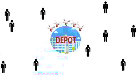
Figure 2. An example of the locations of the central depot and the patients.

Table 1. Formulation of the UCVRP.

Sets	$V$: Set of vertices where $V=\left\{v_0, v_1, \dots ,v_n\right\}$ $E$: Set of edges $\left(e\in E\right)$ $U$: Set of UAVs $\left(u\in U\right)$ $R_k$: Set of vertices visited by UAV $u_k$
Parameters	$v_0$: A central depot of starting and ending routes for each UAV $v_i$: Location of patient $i$ $e_{ij}$: The flight distance between $v_i \mathrm{and} v_j$, $i\ne j$ $q$: Amount of capacity of each UAV $d_i$: Weight of blood needed by $v_i$ $w_i$: Weight of the required water to deliver blood to patient $i$ $m$: Total number of UAVs used in the solution $($m$\le \left|U\right|)$ $n$: Total number of patients $\left(n=\left|V\right|\right)$ $b_{ij}$: Battery consumed on one trip between $v_i \mathrm{and} v_j$ ${\mu }_t$: The UAV mass tare without battery and load, i.e., UAV mass ${\mu }_b$: The UAV battery mass $\theta s$: Lift-to-drag ratio η: The efficiency of the power transfer
Decision variables	$x_{ijk}=\{\begin{array}{c}1, \mathrm{if} u_k \mathrm{flies} \mathrm{from} v_i \mathrm{to} v_j\hfill \\ 0, \mathrm{otherwise}\hfill \end{array}$	(1)
	$y_{ik}=\{\begin{array}{c}1, \mathrm{if} u_k \mathrm{serves} v_i\hfill \\ 0, \mathrm{otherwise}\hfill \end{array}$	(2)
Objective function	$Minimize Z={\displaystyle \sum }_{i=0}^n{\displaystyle \sum }_{j=0}^n{\displaystyle \sum }_{k=1}^m{e}_{ij}·x_{ijk}$	(3)
	$Minimize m$	(4)
Constraints	${\displaystyle \sum }_{i=1}^n\left(d_i+w_i\right)·y_{ik}\le q,\forall k$	(5)
	${\displaystyle \sum }_{k=1}^m{x}_{0jk}\le m, \forall j$	(6)
	${\displaystyle \sum }_{k=1}^m{y}_{ik}=1, \forall i, i\ne 0$	(7)
	${\displaystyle \sum }_{i=0}^n{x}_{ijk}=y_{jk}, \forall j, j\ne 0, i\ne j, \forall k$	(8)
	$R_{k1}{{\displaystyle \cap }}^{ }{R}_{k2}=\left\{v_0\right\}, \forall k1,\forall k2$	(9)
	$\underset{k}{\cup }{R}_k=\left\{v_0, v_1, \dots ,v_n\right\}$	(10)
Assumptions	Following the model in [27], the following is assumed: All UAVs are of the same type. We do not consider the impact of environmental factors, e.g., weather and terrain topology conditions. bij, i.e., the battery needed by patient j, is given by Equation (12) [28]. μt, μb, θs, and η are fixed for all UAVs, so we treat them as constants.

Formally, the UCVRP is an NP-hard combinatorial optimization problem. The solutions in combinatorial optimization problems are encoded with discrete variables. The UCVRP was formulated by Wen et al. [10] as a graph $G=(V,E$, where $V=\{v_1$,$v_2$, …,$v_n\}$ is a set of vertices; $v_0$ represents the depot (i.e., blood warehouse), which is a starting and ending point for each UAV; $v_1$,$v_2$,…,$v_n$ are the locations of patients; and $E$ is a set of edges between vertices ($e_{ij}$ is the traveling distance between$v_i$ and$v_j$). Each patient $i$ has a blood demand$d_i$. $U$ is a set of UAVs. Each UAV has a restricted load capacity $q$. UAVs with a limited capacity are responsible for transporting blood to patients. The blood temperature must remain in the range of 2–10 °C during transportation (i.e., according to the weather and environment, hot water or ice must be stored with the blood bags to keep the blood temperature within the prescribed range). The total demand weight of patient $i,$ $t_i,$ is the total weight of the required blood with the amount of water needed to keep the blood viable, as calculated by Equation (11):

$$t_i=d_i+w_i$$

(11)

There are two decision variables of the Boolean type: $x_{ijk}$ (1) and $y_{ik}$ (2). The objectives are to minimize the total traveling distance of UAVs $Z$ (3), and the number of UAVs used $m$ (4). Constraint (5) ensures that in each individual route, the total patient demands must be less than or equal to the UAV’s capacity $q$. Constraint (6) guarantees that the total number of UAVs used should not exceed $m$. Constraint (7) ensures that each patient is served by only one UAV. Constraint (8) ensures that each patient must be served only once. Constraint (9) ensures that there is only a single depot for all UAVs. Constraint (10) guarantees that all patients should be served. Together, Constraints (7)–(10), guarantee that each UAV launches from and returns to the depot, i.e., each route forms a loop.

Equation (12) calculates $b_{ij}$, i.e., the battery needed by patient $j$ [28], where a UAV travels to $v_j$ with a load $t_j$:

$$b_{ij}=\frac{{\mu }_t+{\mu }_b+t_j}{\theta s \eta }\times e_{ij}$$

(12)

4. Solution Method

This paper proposes a novel heuristic known as the GBDOH to solve the UCVRP. The objective of the UCVRP is to minimize the total routes (i.e., the number of UAVs) and the total distance. The GBDOH satisfies all of the constraints in Table 1. At the outset, the idea of the heuristic contains two main processes described in Algorithms 1 and 2. Algorithm 1 (i.e., find the initial solution) is used for selecting suitable patient demand weights (blood and water) that do not exceed the UAV’s capacity, while minimizing the number of operated UAVs. Algorithm 2 (i.e., improve the initial solution) enhances (i.e., minimizes) the total distance of the initial solution. Figure 3 shows a high-level flowchart of the GBDOH followed by an explanation for each algorithm.

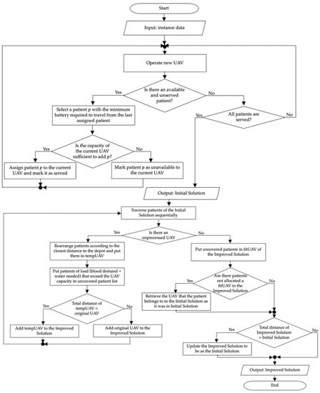
Figure 3. Flowchart of the GBDOH.

4.1. Find Initial Solution

The idea is to build routes (i.e., assign patients to UAVs) according to the lowest battery consumption to operate as few UAVs as possible, i.e., if $i$ is a current patient, we choose the next patient $j$ with the lowest battery consumption ($b_{ij}$) from$i$.

First, the input is an instance file containing the number of patients, UAV capacity, depot and patient locations, and blood demand weight of each patient. Then, operate a new UAV $u$ and sort unserved patients $p\in P,$ where $P\subset V,$ in ascending order according to the battery power needed to reach each of them from the depot by$u,$ i.e., $b_{v_{0}p}$, $p\in P$, as shown in Equation (12), where the distance and the demand (blood and water) are variables. From the list of unserved patients, select patient $p_m$ with the minimum $b_{v_0{p}_m}$, assign it to $u$ and mark it as served, then make it as current patient $p_c$. Then, sort unserved patients $p\in P$ in ascending order according to $b_{p_{c}p}$, considering the mass of water needed to keep the blood usable according to the cumulative distance starting from the depot, i.e., from the depot to patient $p\in P$ via all the assigned patients to this UAV and preceding $p$. After that, choose patient p_m from the available and unserved patients with the lowest $b_{p_c{p}_m}$. Then, we check the available capacity of $u$ to see if it is possible to combine the blood demand of $p_m$ with the water needed for preservation before assigning $p_m$ to the current UAV ($u$) and marking them as current patient $p_c$; otherwise, mark $p_m$ as unavailable to add to this UAV, and perform the process again to choose another $p_m$ as mentioned above; this process is repeated until finishing all available patients. If all patients are served or the current UAV $u$ is not available to add more patients, operate a new UAV $u$ and repeat the processes above. Otherwise, the process ends.

Algorithm 1. Find initial solution
1	P ← List of all potential patients ⊂ V
2	U ← Set of the available UAVs
3	Total_distance ← 0
4	Initial_solution ← { }
5	dist ← List of distances from depot to each patient p, dist ⊂ E
6	Calculate $b_{v_0 p}=\left(d_p+w_{dist\left[p\right]}\right)\ast dist\left[p\right] \forall p\in P$ \\The battery consumed from depot for all patients
7	\\Build the solution: the routes (trips for the needed UAVs) and the total distance
8	p ← 0
9	Repeat
10	Select (new u ∈ U)
11	pm←Min(available P)\\according to minimum $b_{v_{0}p} \forall p\in P$ (the minimum battery consumed from depot)
12	rd←$dist\left[p_m\right]$ \\rd is the route distance of the current UAV u
13	Assign_to_UAV (u, pm)
14	MarkAsServed(pm, P)
15	Increment p
16	pc ← pm \\current patient
17	\\Add other patients to the route (UAV)
18	end_route = False
19	While (end_route = = False)
20	cumulative_dist ←List of distances from pc to p +rd ∀ p ∈ available P
21	\\The battery consumed from pc to all available patients
22	Calculate $b_{p_{c}p}$ = (dp + wcumulative_dist[p]) ∗ cumulative_dist [p] ∀ p ∈ availableP
23	found = False
24	pm← −1
25	\\Find next candidate patient
26	While (found = = False AND p < size of P)
27	pm← Min($b_{p_{c}p}$) \\p ∈ available P
28	IF pm ≠ −1 Then \\route does not end
29	IF capacity of the UAV u is available to add pm Then
30	Assign_ to_UAV(u, pm)
31	MarkAsServed(pm, P)
32	rd ← cumulative_dist [pm]
33	$p_c$← pm \\ current patient
34	Increment p
35	Found ← True
36	Else
37	MarkAsUnavailable(pm, u)
38	Else
39	end_route ← True
40	break
41	IF p = = size of P Then \\ if all patients are sarved
42	end_route ← True
43	Total_distance ← Total_distance + rd
44	Initial_solution ← Initial_solution ∪ u
45	Until U times OR all patients in P are served
46	Output: Initial_solution, Total_distance

4.2. Improve the Initial Solution

The idea here is to rearrange each route (the patients assigned to UAVs, i.e., the output of Algorithm 1) of the initial solution according to the shortest distance from the depot in order to minimize the total consumed distance.

First, traverse the UAVs (routes) of the $initial\_solution$ one by one until completion, and carry out the subsequent steps for each round. Then, create a new temporary UAV, $tempUAV$, to keep the patients of the current UAV after sorting them based on distance. After that, sort the assigned patients of the current UAV, $u$, in ascending order according to the distance, $dist$, from the depot. Then, select patient$c$ with the lowest flight distance $e_{v_{0}c}$, add them to $tempUAV$ as the first patient, and mark them as an arranged patient and $p_c$. If the unarranged list of patients in the current UAV, $u$, is not empty, select patient $c$ with the smallest distance from the last arranged patient$p_c$, i.e., $e_{p_c. c}$. Then, check the availability of the $tempUAV$ capacity; if it is available to add the blood demand of $c$ along with the mass of water required to keep the blood usable, according to the cumulative distance starting from the depot to the patient$c$, then add $c$ to $tempUAV$, mark them as an arranged patient and as $p_c$, and select another patient $c$; otherwise, remove $c$ from $u$, add them to the unserved list ($uncoverd)$, save $u$’s ID, and select another patient $c$. If the total distance of $tempUAV$ is less than the total distance of the current UAV, $u$, add $tempUAV$ to the $improvedSolution$; otherwise, discard $tempUAV$ and add the current UAV, $u$, to the $improvedSolution$ (i.e., keep the current route as it was in the initial solution).

Go to the next UAV from the $initial\_solution$ and repeat the above processes again until all UAVs are traversed.

Traverse the unserved patients $p_u ϵ uncovered$ one by one until completion and do the following. Find a UAV $fitUAV$ from the $improvedSolution$ whose capacity is available to add the current unserved patient $p_u ϵ uncovered$, and the total route distance of $fitUAV$ (after adding$p_u$) will be the shortest compared with the other available UAVs of the $improvedSolution$. If there is no UAV available to add $p_u$, or if the total distance of the $improvedSolution$ after adding $p_u$ to $fitUAV$ will be greater than the total distance of the $initial\_solution,$ then change the route in the $improvedSolution$ of the UAV, $original\_UAV$ (to which the patient was assigned in the$initial\_solution$), to be as it was in the $initial\_solution$, and clear all unserved patients in $uncovered$ that came from the same UAV. Additionally, retrieve all other routes that took patients from $original\_UAV$ as they were in the $initial\_solution$. Otherwise, assign $up$ to $fitUAV$.

Algorithm 2. Improve the initial solution
1	Input: Initial_solution, Total_distance
2	improvedSolution ← { }
3	changed_routes_IDs ← { }
4	Total_distance ← 0
5	For each UAV u in Initial_solution Do
6	tempUAV ← new UAV
7	uncovered_1 ← { } \\To keep uncovered patients of the current route (UAV level)
8	uncovered_2 ← { } \\To keep uncovered patients by the improved solution (solution level)
9	All_covered ← True
10	Route_distance ← 0
11	\\First patient
12	FindClosest (v0, c) \\Find the closest patient C to the depot from UAV u
13	Assign_to_UAV(tempUAV, c)
14	$Route\_distance\leftarrow Route\_distance+e_{v_0 c}$
15	MarkAsUnavailable(c, tempUAV)
16	current_patient ← c
17	\\Rearrange other patients of the UAV u according to the shortest closest neighbor
18	i ← 1
19	While(i < number of patients of u)
20	FindClosest(pc, c)
21	IF capacity of tempUAV is available to add C Then
22	Assign_to_UAV(tempUAV, c)
23	$Route\_distance\leftarrow Route\_distance+e_{p_c C}$
24	pc ← c
25	MarkAsServed(c)
26	Else
27	All_covered ← False
28	uncovered_1 = uncovered_1 ∪ c
29	MarkAsUnavailable(c, tempUAV)
30	Increment i
31	IF tempUAV < urouteDistance Then \\The route distance is improved
32	improvedSolution = improvedSolution ∪ tempUAV
33	IF size(uncovered_1) > 0 Then
34	uncovered_2 = uncovered_2 ∪ uncovered_1
35	Else
36	improvedSolution = improvedSolution ∪ u\\Keep UAV as in initial solution
37	Total_distance ← Total_Distance + route_distance
38	\\add uncovered patients
39	IF size(uncovered_2) > 0 Then
40	For each uncovered patient pu in uncovered_2 Do
41	originalUAV ← UAV from initial_solution that pu was assigned to
42	fitUAV ← −1
43	fitUAV ← UAV d from improvedSolution of available capacity to add pu with minimum route distance
44	changed_routes_IDs ← changed_routes_IDs ∪ original_UAV
45	IF fitUAV ≠ −1 Then
46	IF the total distance of improvedSolution after adding pu to fitUAV <the total distance of Initial_solution Then
47	Total_distance ←the total distance of $improvedSolution$ after adding pu to fitUAV
48	changed_routes_IDs ← changed_routes_IDs ∪ Fit_UAV
49	Else
50	improvedSolution[original_UAV] ← initial_solution[original_drone]
51	Else
52	For each chr in changed_routes_IDs Do
53	improvedSolution[chr] ← initial_solution[chr]
54	Clear other patients from uncovered_2 who are assigned to original UAV in the initial solution
55	Output: improvedSolution

5. Experimental Results

This section describes the dataset used to test the proposed GBDOH, and then presents a detailed numerical analysis of the results.

The GBDOH was implemented using Python software. The experiments were conducted using a computer with an Intel Core i7 processor running at 3.1 GHz using 16 GB 2133 MHz LPDDR3 of RAM running Macintosh HD.

5.1. Dataset

For the sake of comparison, we tested the GBDOH on instances of the CVRP public dataset (Christofides and Eilon, Set E) benchmark [29] used in the related work [10]. Each instance is described by a notation that contains the characteristics of that instance: E-nx-ky, where the symbol ‘E’ stands for Eilon et al., who were the creators of the dataset, ‘nx’ is the number of the demands of the instance (i.e., patients), and ‘ky’ is the minimum number of trucks of the exact solution (UAVs). The tested instances were E-n23-k3, E-n30-k3, E-n22-k4, E-n30-k4, E-n33-k4, E-n51-k5, E-n76-k7, E-n76-k8, E-n76-k10, E-n76-k14, E-n101-k8, and E-n101-k14. To measure the average performance for different sizes of the problem, we divided the instances into three categories according to the number of patients $n$ (depending on the range of patients that we observed in the dataset, which was 20–101)—small ($n<50$), medium ($50\le n<100$), and large ($100<n$)—and calculated the average of the objective function for each category.

To extract the ratio that determines the amount of water needed from Table 2, we mapped the required weight of blood and the distance to the patient to the range [0, 20] according to Equations (13) and (14), as adjusted by [10]. For example, according to Table 2, when the flight distance to a patient is 3 units and the demanded weight of blood is 12 units, the ratio is 0.03; thus, the weight of water needed is 12 × 0.03.

$$bloodCoord=20\times \frac{bloodWeight-minBlood}{maxBlood-minBlood}$$

(13)

$$distanceCoord=20\times \frac{distance-minDistance}{maxDistance-minDistance}$$

(14)

Table 2. The ratio between blood and water [10].

Distance to Patient	Blood Weight
	[0, 2]	[2, 3]	[3, 5]	[6, 10]	[10, 15]	[15, 20]
[0, 5]	1	0.5	0.2	0.06	0.03	0.02
[5, 10]	1.2	0.8	0.4	0.10	0.06	0.04
[10, 15]	1.9	1.2	0.6	0.18	0.12	0.08
[15, 20]	2.4	1.5	0.8	0.28	0.18	0.15

In Equation (13), $bloodCoord$ is the value of the demanded weight of blood after mapping to 20, while $minBlood$ is the minimum possible demanded weight of blood in a dataset instance, which equals 0. Additionally, $maxBlood$ is the maximum one demanded weight. To avoid exceeding the carrying capacity of the UAV, we set $maxBlood,$ as shown in Equation (15):

$$maxBlood=\frac{\mathrm{the} \mathrm{maximum} \mathrm{demand} \mathrm{weight} \mathrm{of} \mathrm{blood} \mathrm{from} \mathrm{dataset}}{\left(1+0.2\right)}$$

(15)

In Equation (14), $distanceCoord$ is the value of the distance after mapping to 20. The $minDistance$ is the minimum flight distance that can be set directly for any data instance; here, we set it once to 50 and another time to 100 for each instance to compare the results with those reported in [10]. We set $maxDistance$ as the maximum distance from the distance matrix of an instance dataset.

Unlike the approach of [10], which is a population-based method and deals with the problem as a multi-objective one, our approach is a single-solution-based method and deals with the problem as a single-objective problem. To extract the objective value, we proceeded as follows:

• Run the heuristic on each instance.
• Normalize both the (i) number of routes (UAVs) and (ii) distance to a $\left[0,1\right]$ interval for each.
• Give weights for the normalized number of routes (UAVs) and distance, which indicate the importance of each term.
• Merge them into a single value that represents the objective value (i.e., single objective).

The following are the equations and parameters used to extract the objective value. The min–max normalization equation is as follows [30]:

$$\frac{x-min\left(x\right)}{max\left(x\right)-min\left(x\right) }\times \left(new max-new min\right)+new min$$

(16)

For the number of UAVs, we use Equation (16) as follows: Suppose that $x$ is the number of routes (UAVs) before normalization; $min\left(x\right)$ is the baseline number of UAVs, which is the number of trucks taken from the instance file; and$max\left(x\right)$ is adjusted based on historical data observed in our work and the related work [10]. The $max\left(x\right)$ is adjusted to 7, 26, and 30 for small, medium, and large size instances, respectively.

For the distance, we use Equation (16) as follows: Suppose that $x$ is the distance before normalization. $min\left(x\right)$ is the baseline distance, which is adjusted based on historical data observed in our work, the related work [10], and the instance file. The $min\left(x\right)$ is adjusted to 370, 520, and 810 for small, medium, and large instance sizes, respectively.$max\left(x\right)$ is adjusted based on historical data observed in our work, the related work [10], and the instance file. The $max\left(x\right)$ is adjusted to 1320, 1610, and 2020 for small, medium, and large distances, respectively.

The $new max \mathrm{and} new min$ are 1 and 0, respectively, since we intend to normalize to $\left[0, 1\right]$ intervals.

For the objective values, we give weights of 0.5 for the normalized number of UAVs and 0.5 for the normalized distance, add them, and divide the sum by 2, as shown in Equation (17):

$$Objective Value=\frac{\left(0.5\times \mathrm{the} \mathrm{normalized} \mathrm{no}. \mathrm{of} \mathrm{UAVs}\right)+\left(0.5\times \mathrm{the} \mathrm{normalized} \mathrm{distance}\right)}{2}$$

(17)

In [10], the authors generated a Pareto optimal set with a tradeoff between the two objectives. To compare our results with the previous work [10], we applied the above steps to their results to convert the objective values to a single-objective function. We then compared our work with theirs. The next section provides a detailed explanation of the results and comparison.

5.2. Numerical Analysis

This study features a new heuristic (GBDOH) to solve the UCVRP [10]. We compared the results of the GBDOH with those of the MOEA/D-N-UVRP [10] to obtain the smallest number of UAVs within the shortest possible distance.

In terms of the number of UAVs used and the distance, the algorithm that accomplished the best results in [10] was the MOEA/D-N-UVRP. Section 2 explains that the MOEA/D-N-UVRP involves evolutionary algorithms and local search. In the evolutionary algorithm, random solutions are initialized before operations such as crossover and mutation are iteratively applied to them to generate new solutions. In the local search, the MOEA/D-N-UVRP applies the random nearest neighbor search to enhance the solution obtained by the evolutionary algorithm. However, the local search does not always enhance the solution. Moreover, each run gives a different solution, so we cannot guarantee the best solution provided by the algorithm.

In summary, the main difference between the GBDOH and the work in [10] is that the GBDOH progresses from a single solution method, while the work in [10] uses a population-based solution method (i.e., an evolutionary algorithm). In addition, the GBDOH uses two phases to solve the problem: The first phase works to obtain a solution that has the smallest possible number of routes (UAVs), by adding patients to each UAV who require the least battery for blood delivery compared with other patients. The second phase works to rearrange the order of patients in each route to minimize the distance while satisfying the problem constraints. On the other hand, the work in [10] used a multi-objective approach to solve the UCVRP and did not consider the battery consumption to minimize the number of routes.

5.2.1. Comparisons of the Results of the GBDOH and MOEA/D-N-UVRP

Table 3 shows the results of the GBDOH and MOEA/D-N-UVRP on 20 cases of nine different instances stated in [10] and in Section 5.1. In Table 3, the instances are grouped by the size of the instance, which depends on the number of patients (small, medium, or large). The table shows the baseline values of UAVs and the distances reported in the solutions of the benchmark instances. For each use of the MOEA/D-N-UVRP and GBDOH, Table 3 shows the number of UAVs (routes) and the distances before and after normalization, along with the objective value for each instance. It also shows the average of these items based on the instance size. In addition, Table 3 reports the average run time of each instance tested by the GBDOH. The bold typeface signifies better values.

Table 3. Comparison between the MOEA/D-N-UVRP and GBDOH, the bold font indicates best values for each instance.

					MOEA/D-N-UVRP					GBDOH
Size	Instance	Baseline Routes	Baseline Distance	Minimum Distance	Routes (UAVs)	Distance	Normalized Number of Routes	Normalized Distance	Objective Value	Routes (UAVs)	Distance	Normalized Number of Routes	Normalized Distance	Objective Value	Run Time (Seconds)
Small	E-n23-k3	3	569	50	5	716.03	0.50	0.36	0.43	5	836.00	0.50	0.49	0.50	0.0011
		3	569	100	5	720.35	0.50	0.37	0.43	5	862.00	0.50	0.52	0.51	0.0013
	E-n30-k3	3	534	50	7	774.98	1.00	0.43	0.71	5	784.00	0.50	0.44	0.47	0.0012
		3	534	100	7	766.82	1.00	0.42	0.71	5	879.00	0.50	0.54	0.52	0.0020
	E-n22-k4	4	375	50	7	562.32	1.00	0.20	0.60	5	548.00	0.50	0.19	0.34	0.0008
		4	375	100	7	552.64	1.00	0.19	0.60	5	583.00	0.50	0.22	0.36	0.0010
	E-n30-k4	4	503	50	7	555.97	1.00	0.20	0.60	5	784.00	0.50	0.44	0.47	0.0024
		4	503	100	7	555.81	1.00	0.20	0.60	5	879.00	0.50	0.54	0.52	0.0014
	E-n33-k4	4	835	50	7	563.07	1.00	0.20	0.60	6	1291.00	0.75	0.97	0.86	0.0020
		4	835	100	7	553.94	1.00	0.19	0.60	6	1253.00	0.75	0.93	0.84	0.0016
Average					6.6	632.19	0.90	0.28	0.59	5.2	869.90	0.55	0.53	0.54	0.0015
Medium	E-n51-k5	5	521	50	14	929.48	0.43	0.38	0.40	6	781.00	0.05	0.24	0.14	0.0046
		5	521	100	13	931.32	0.38	0.38	0.38	7	878.00	0.10	0.33	0.21	0.0049
	E-n76-k7	7	683	50	19	1594.25	0.67	0.99	0.83	8	1011.00	0.14	0.45	0.30	0.0081
		7	683		20	1326.82	0.71	0.74	0.73	8	1011.00	0.14	0.45	0.30	0.0081
		7	683	100	19	1359.27	0.67	0.77	0.72	8	1216.00	0.14	0.64	0.39	0.0103
		7	683		20	1347.64	0.71	0.76	0.74	8	1216.00	0.14	0.64	0.39	0.0103
	E-n76-k14	14	1032	50	26	1599.41	1.00	0.99	1.00	16	1445.00	0.52	0.85	0.69	0.0106
		14	1032	100	26	1593.08	1.00	0.98	0.99	18	1587.00	0.62	0.98	0.80	0.0128
Average					19.625	1335.16	0.70	0.75	0.72	9.875	1143.13	0.23	0.57	0.40	0.0086
Large	E-n101-k14	14	1077	50	30	1942.28	1.00	0.81	0.91	16	1681.00	0.36	0.72	0.54	0.0130
		14	1077	100	30	1929.00	1.00	0.81	0.90	19	2000.00	0.50	0.98	0.74	0.0146
Average					30	1935.64	1.00	0.81	0.90	17.5	1840.50	0.43	0.85	0.64	0.0138
Total Average					14.15	1043.72	0.83	0.52	0.67	8.3	1076.25	0.41	0.58	0.49	0.0052

Figure 4 compares the average results of each group size of instances tested by the GBDOH and MOEA/D-N-UVRP in terms of objective value, route % (i.e., percent deviation from the value of the baseline routes), and distance % (i.e., percent deviation from the value of the baseline distance).

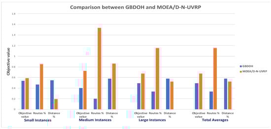
Figure 4. Comparison between the average results of the GBDOH and MOEA/D-N-UVRP on each group size of instances in terms of objective value, percent deviation from the value of the baseline routes, and percent deviation from the value of the baseline distance.

According to Table 3 and Figure 4, the GBDOH has a better objective value than MOEA/D-N-UVRP with respect to the average instance size (i.e., improvement in small instances by 8.5%, medium instances by 44.3%, and large instances by 29%), as well as improving the total average of all instances by approximately 27%. However, the MOEA/D-N-UVRP has better distances (minimum distances) than the GBDOH in most cases. The reason behind the preponderance of objective values of the GBDOH is the limited number of routes (UAVs) used, which is a benefit of using the battery consumed as a factor when assigning patients to a UAV.

Figure 5 shows the best objective values obtained by the GBDOH and MOEA/D-N-UVRP using the nine instances from the Christofides and Eilon, Set E benchmark [29]. The GBDOH has better (minimum) objective values than the MOEA/D-N-UVRP in seven out of nine tested instances in which $minDistance$= 50.

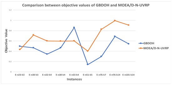
Figure 5. Comparison between the objective values of the GBDOH and MOEA/D-N-UVRP on nine instances from the (Christofides and Eilon, Set E) benchmark.

To guarantee that the analysis relied on a solid statistical basis, we compared the objective values obtained by the GBDOH and MOEA/D-N-UVRP by applying the Wilcoxon signed-rank test as follows: The null hypothesis was that the population distributions of the GBDOH and MOEA/D-N-UVRP would be identical with respect to the objective values. The results showed that there were 16 negative and 4 positive ranks. Accordingly, most pairs were negative, meaning that the GBDOH outperformed the MOEA/D-N-UVRP in terms of objective values. Moreover, the $p$-value = 0.00318, where 0.00318 < 0.05; consequently, the null hypothesis was rejected. Thus, we can conclude that the GBDOH is better than the MOEA/D-N-UVRP with respect to objective values.

The GBDOH endeavors to outperform the MOEA/D-N-UVRP by focusing on elements that minimize the number of UAVs used and the total distance simultaneously, using fewer and more efficient processes in a greedy deterministic manner. To this end, in the initial solution of the GBDOH, a patient $j$ with a minimal amount of required UAV battery $b_{ij}$ is assigned to the UAV. This approach works by reducing the amount of battery consumed by the UAV to serve patients, allowing the UAV to serve a large number of patients and minimizing the number of operated UAVs. In addition, this approach may also reduce the travel distance, since the amount $b_{ij}$ is based on two principal factors: weight and distance. Furthermore, the GBDOH aims to improve the initial solution by rearranging the order of patients based on a greedy closest-distance patient process without operating new UAVs, as explained in Section 4. This helps to accomplish the objective of minimizing the total distance. Thus, these features are the reason that the GBDOH outperforms the MOEA/D-N-UVRP.

Moreover, with respect to the computational time, our algorithm was fast, with an average runtime of 0.0052 s, as shown in Table 3. The reason for this could be that it focuses on a single solution and uses greedy deterministic methods. In contrast, the authors of [10] tried to solve the UCVRP using a method that combines an evolutionary algorithm with a local search method. The evolutionary algorithm primarily relies on blind operators (i.e., crossover and mutation); subsequently, the search process may return prematurely after converging to a locally optimal solution. Additionally, the evolutionary algorithm is one of the population-based metaheuristics, which are known in the literature for their slow processing time—especially given that the authors of [10] used a population size = 100 and a number of iterations = 15,000,000. We provide more details on the comparison of computational complexity between the GBDOH and MOEA/D-N-UVRP in Section 5.2.2.

Finally, Figure 6 and Figure 7 display the initial and improved solutions, respectively, when testing the GBDOH on instance E-n101-k14. The colors are used to distinguish the routes. The numbers are patients. Table 4 shows the details of the routes and distances. The left-hand side of the table shows the number of nodes of each route, the distance of each route, and the total distance of the initial solution. The right-hand side shows the same details but for the improved solution. The bold font indicates values that offer improvements from the initial solution to the improved solution.

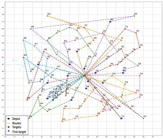
Figure 6. Initial solution of the GBDOH for instance E-n101-k14.

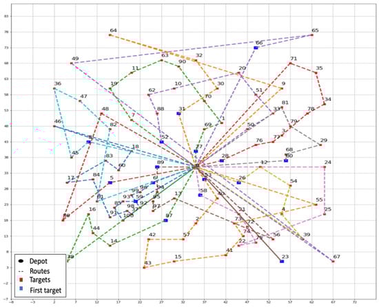
Figure 7. Improved solution of the GBDOH for instance E-n101-k14.

Table 4. Initial and improved solutions of the GBDOH for instance E-n101-k14.

Instance E-n101-k14
Initial Solution		Improved Solution
Routes	Route Distance	Routes	Route Distance
Route #1: {0, 91, 92, 37, 98, 99, 96, 6, 60, 83, 46, 17, 84, 18, 0}	131	Route #1: {0, 6, 96, 99, 92, 37, 98, 91, 84, 17, 83, 60, 18, 46, 0}	125
Route #2: {0, 53, 40, 2, 57, 42, 43, 15, 41, 74, 73, 55, 0}	123	Route #2: {0, 53, 40, 2, 57, 42, 43, 15, 41, 74, 73, 55, 0}	123
Route #3: {0, 27, 69, 1, 70, 90, 63, 11, 19, 7, 0}	88	Route #3: {0, 27, 69, 1, 70, 90, 63, 11, 19, 7, 0}	88
Route #4: {0, 28, 76, 77, 3, 78, 34, 35, 71, 0}	93	Route #4: {0, 28, 76, 77, 3, 78, 34, 35, 71, 0}	93
Route #5: {0, 52, 88, 62, 10, 20, 51, 33, 50, 0}	88	Route #5: {0, 52, 88, 62, 10, 20, 51, 33, 50, 0}	88
Route #6: {0, 89, 97, 95, 94, 13, 56, 0}	88	Route #6: {0, 89, 94, 95, 97, 13, 56, 0}	84
Route #7: {0, 58, 21, 72, 75, 22, 25, 24, 0}	100	Route #7: {0, 58, 21, 72, 75, 22, 25, 24, 0}	100
Route #8: {0, 80, 68, 29, 79, 81, 0}	75	Route #8: {0, 80, 68, 29, 79, 81, 0}	75
Route #9: {0, 26, 12, 54, 4, 39, 0}	79	Route #9: {0, 26, 12, 54, 4, 39, 0}	79
Route #10: {0, 8, 45, 36, 47, 82, 61, 0}	120	Route #10: {0, 8, 45, 36, 47, 82, 61, 0}	120
Route #11: {0, 100, 93, 59, 85, 0}	61	Route #11: {0, 59, 93, 85, 100, 0}	52
Route #12: {0, 31, 30, 32, 64, 9, 0}	136	Route #12: {0, 31, 30, 32, 64, 9, 0}	136
Route #13: {0, 87, 14, 44, 16, 38, 0}	103	Route #13: {0, 87, 14, 44, 16, 38, 0}	103
Route #14: {0, 5, 86, 48, 0}	100	Route #14: {0, 5, 86, 48, 0}	100
Route #15: {0, 66, 65, 49, 67, 0}	243	Route #15: {0, 66, 65, 49, 67, 0}	243
Route #16: {0, 23, 0}	72	Route #16: {0, 23, 0}	72
Total Distance	1700	Total Distance	1681

In Table 4, we can observe the improvement of the distances of Route#1, Route#6, and Route#11 without adding more UAVs. The total distance of the complete solution decreases from 1700 to 1681 after applying the improved solution algorithm.

5.2.2. Comparison of the Computational Complexity of the GBDOH and MOEA/D-N-UVRP

In the MOEA/D-N-UVRP [10], the key computational costs are as follows:

• Generate $n$ random trail solutions, i.e., population, $O\left(n\right)$.
• The number of generations $g,$ i.e., iterations $O\left(g\right)$ to carry out the following steps:

  ∘

  Crossover is $O\left(p\right)$, where $p$ is the number of patients.

  ∘

  Mutation is $O\left(p\right)$.

  ∘

  The random nearest neighbor search requires $O\left(\frac{p^2}{m}\right)$ operations, where $m$ is the number of UAVs used.

Thus, the time complexity of the MOEA/D-N-UVRP is $O\left(\frac{ng{p}^2}{m}\right)$.

In contrast, in the GBDOH, the major computational costs are as follows:

• The algorithm to find the initial solution requires $O(m{p}^2$), where $m$ is the number of UAVs used and $p$ is the number of patients. $O\left(m{p}^2\right)$ is derived from the worst-case performance of Algorithm 1, where it consists of a main loop (outer loop) along with two nested (inner) loops. The outer loop spans from line 9 to line 45. The first inner loop spans from line 19 to line 42, while the second spans from line 26 to line 40. The inner loop that takes the longest time (in the worst case) is on line 26, where it takes $O(p)$. Thus, the outer loop (Repeat-until) that is on lines 9–45 takes $O\left(m{p}^2\right)$.
• The algorithm to improve the initial solution requires $O(m{r}_p^2$), where $r_p$ is the number of patients in the route, i.e., $r_p<p$. $O(m{r}_p^2$) is derived from the worst-case performance of Algorithm 2, where it consists of main loop (outer loop) from line 5 to line 37, along with a nested (inner) loop from line 19 to line 30. The inner loop takes in the worst case $O(r_p^2$). Thus, the outer loop on lines 5–37 takes $O\left(m{r}_p^2\right).$
• Thus, the time complexity of the GBDOH is $O(m{p}^2$).

Therefore, if the GBDOH and MOEA/D-N-UVRP have the same number of patients $p$ and UAVs used $m$, then the ratio between their computational complexities is as follows:

$$\frac{O\left(m{p}^2\right)}{O\left(\frac{ng{p}^2}{m}\right) }=\frac{O\left(m^2\right)}{O\left(ng\right) }$$

The parameter values used in [10] were $n$ = 100 and $g$ = 15,000,000. Consequently, since $m^2$ is smaller than $n\times g$ = 1,500,000,000, the GBDOH has lower computational complexity than the MOEA/D-N-UVRP.

5.2.3. Experiments on the XML100 Benchmark Dataset

To validate the benefit of the algorithm in improving the initial solution, and to further test the efficiency of our heuristic, we conducted experiments on 2844 instances of a new benchmark dataset of the CVRP named XML100, released in 2021 [29]. The tested instances comprise 108 groups based on their categories. The categories are as follows: depot positioning (centered), customer positioning (random, clustered, and random-clustered), demand distribution (small values with large CV, small values with small CV, large values with large CV, large values with small CV, values depending on quadrant, and numerous small values with few large values, where CV denotes the capacity of the vehicle), and average route size (very short, short, medium, long, very long, and ultra-long). Each instance comprises 100 customers. The tables in Appendix A show the details of the initial solution, the improved solution, the time of the whole process when applying the GBDOH on the XML100 dataset, and the improvement shown as a percentage. The bold font indicates values that offer improvements from the initial solution distance to the final solution distance.

Table A1 groups instance categories by centered depot positioning and random customer positioning in 36 groups, each with 27 instances (totaling 972). According to this table, the average total distance in the improved solution decreases by 2.6%, with a total average time of 0.0109 s and a p-value < 0.00001.

Table A2 groups instance categories by centered depot positioning and clustered customer positioning in 36 groups, each with 26 instances (totaling 936). This table shows that the average total route distance in the improved solution decreases by 2.4%, with a total average time of 0.0107 s and a p-value < 0.00001.

Table A3 groups instance categories by centered depot positioning and random-clustered customer positioning in 36 groups, each with 26 instances (totaling 936). According to this table, the average total route distance in the improved solution decreases by 2.6%, with a total average time of 0.0117 s and a p-value < 0.00001.

Thus, from Table A1, Table A2 and Table A3, we can conclude that in all of these cases the improved solution proves better than the initial solution with respect to the total route distance, helping to achieve better objective values.

The average route distances of the initial solutions of all categories amount to 19,906.78, whereas the total average of the improved solutions amounts to 19,403.88, indicating an improvement of approximately 2.5%. This development shows the improved algorithm’s effectiveness when applied to the initial solution, where the travel distance is decreased to achieve the second objective of minimizing the distance. Moreover, according to the Wilcoxon signed-rank test, the p-value is <0.00001, which makes the improved solution significantly better than the initial solution with respect to the total route distance, and also improves the objective value. Since the UCVRP is a real and NP-hard computational problem—especially in healthcare emergency situations—any small improvement in results will reflect huge cost savings in real settings.

In addition, the short processing time represents another advantage of the GBDOH that requires consideration, since the GBDOH will be used in healthcare emergency situations in which the response time constitutes a significant and critical factor.

Finally, it is worth noting that the results in Table A1, Table A2 and Table A3 provide new benchmark baseline results for other researchers working on the UCVRP to test their approaches and compare their results, in addition to the few instances tested in [10].

6. Conclusions

Healthcare services can be improved by utilizing UAVs to deliver blood to patients in emergency scenarios. This study sought to provide high-quality solutions for the UAV-based Capacitated Vehicle Routing Problem (UCVRP) in a reasonable time. The UCVRP is more complex than the traditional CVRP, as it requires additional constraints related to the UAV and blood viability conditions. The objective is to minimize the number of UAVs used and the total distance traveled by the UAVs. The best state-of-the-art approach to solve this problem is the MOEA/D-N-UVRP described in [10]. This multi-objective evolutionary algorithm offers a local search method. However, using multiple objectives and the nature of evolutionary algorithms and local search often requires numerous computations to find a solution. Moreover, the solution varies in each run due to the stochastic nature of the algorithm, meaning that it is not certain to obtain the best solution for each run. Since the problem focuses on helping patients in emergency situations, ensuring a quality solution within a reasonable time proves critical in quickly responding to emergency situations.

In this paper, we propose a new deterministic heuristic known as the Greedy Battery—Distance Optimizing Heuristic (GBDOH) to solve the UCVRP. The GBDOH is distinguished by the following lightweight characteristics: (i) build routes (i.e., assign patients to UAVs) according to the lowest battery consumption in order to operate the fewest UAVs and utilize the UAV capacity effectively, and (ii) rearrange each route (i.e., the patients assigned to the UAVs) according to the shortest distance from the depot in order to decrease the total route distance.

We compared the GBDOH with the state-of-the-art method (MOEA/D-N-UVRP), considering the quality of the solution and time efficiency. For statistical comparison, we utilized the Wilcoxon signed-rank test. The results revealed that the GBDOH has superior solution quality (i.e., the number of UAVs used and total routing distance), where GBDOH enhanced the average objective value by approximately 27% less than MOEA/D-N-UVRP UVRP in an average time of approximately 5.2 ms.

In addition, we tested the GBDOH twice on a new benchmark dataset of the CVRP known as XML100, released in 2021 [29]: (1) using the only initial solution algorithm, and (2) using both the initial solution and the improved solution algorithm. We then compared their results, which showed that when using the improved algorithm the average route distances decreased by approximately 2.5%, while keeping the processing time fast (11.078 milliseconds on average). This enhancement reflects significant cost savings in real settings. Moreover, our research provides new benchmark baseline results for researchers interested in employing the UCVRP to test their methods and compare their results.

In future works, we aim to enhance the GBDOH by changing the appendage to lighter materials than water, so that the UAVs can carry more blood and serve more patients. In addition, we aim to consider obstacle avoidance while minimizing the number of UAVs used and the total routing distance within a short processing time. Moreover, new variations of the problem could be investigated to reflect more realistic healthcare uses, such as visiting charging stations for a UAV’s battery along its journey.

References

- Fukubayashi, Y.; Kimura, M. Improvement of rural access roads in developing countries with initiative for self-reliance of communities. Soils Found. 2014, 54, 23–35. [Google Scholar] [CrossRef]
- Otto, A.; Agatz, N.; Campbell, J.; Golden, B. Optimization approaches for civil applications of unmanned aerial vehicles (UAVs) or aerial drones: A survey. Networks 2018, 72, 411–458. [Google Scholar] [CrossRef]
- Crumley, B. Swoop Aero drones deliver Pfizer COVID-19 vaccines in Malawi—DroneDJ. Available online: https://dronedj.com/2022/03/02/swoop-aero-drones-deliver-ultra-cold-pfizer-covid-19-vaccines-in-malawi/ (accessed on 8 June 2022).
- Dickson, I. Flying pharmacy: Why Medical Drones Will Take Off in 2022. Available online: https://360.here.com/medical-drones (accessed on 8 June 2022).
- Harrisberg, K.; Pensulo, C. From drones to data: New Innovations Are Supporting Africa’s Health Systems. Available online: https://www.weforum.org/agenda/2022/05/drones-to-data-africans-turn-to-healthtech/ (accessed on 8 June 2022).
- Liu, Y. China adapts Surveying, Mapping, Delivery Drones To Enforce World’s Biggest Quarantine And Contain Coronavirus Outbreak | South China Morning Post. Available online: https://www.scmp.com/business/china-business/article/3064986/china-adapts-surveying-mapping-delivery-drones-task (accessed on 27 September 2022).
- Drone First Aid Kit On Blue Stock Illustration 1633656133 | Shutterstock. Available online: https://www.shutterstock.com/image-illustration/drone-first-aid-kit-on-blue-1633656133 (accessed on 30 August 2022).
- Khan, S.I.; Qadir, Z.; Munawar, H.S.; Nayak, S.R.; Budati, A.K.; Verma, K.D.; Prakash, D. UAVs path planning architecture for effective medical emergency response in future networks. Phys. Commun. 2021, 47, 101337. [Google Scholar] [CrossRef]
- Chung, S.H.; Sah, B.; Lee, J. Optimization for drone and drone-truck combined operations: A review of the state of the art and future directions. Comput. Oper. Res. 2020, 123, 105004. [Google Scholar] [CrossRef]
- Wen, T.; Zhang, Z.; Wong, K.K.L. Multi-objective algorithm for blood supply via unmanned aerial vehicles to the wounded in an emergency situation. PLoS ONE 2016, 11, e0155176. [Google Scholar] [CrossRef] [PubMed]
- El-Ghazali, T. Metaheuristics: From Design to Implementation, 2nd ed.; John Wiley & Sons: Hoboken, NJ, USA, 2009; ISBN 9780470278581. [Google Scholar]
- Sajid, M.; Singh, J.; Haidri, R.A.; Prasad, M.; Varadarajan, V.; Kotecha, K.; Garg, D. A Novel Algorithm for Capacitated Vehicle Routing Problem for Smart Cities. Symmetry 2021, 13, 1923. [Google Scholar] [CrossRef]
- Accorsi, L.; Vigo, D. A Fast and Scalable Heuristic for the Solution of Large-Scale Capacitated Vehicle Routing Problems. Transp. Sci. 2021, 55, 832–856. [Google Scholar] [CrossRef]
- Thibbotuwawa, A.; Bocewicz, G.; Nielsen, P.; Banaszak, Z. Unmanned Aerial Vehicle Routing Problems: A Literature Review. Appl. Sci. 2020, 10, 4504. [Google Scholar] [CrossRef]
- Al-rabiaah, S.; Hosny, M.; Almuhaideb, S. An Efficient Greedy Randomized Heuristic for the Maximum Coverage Facility Location Problem with Drones in Healthcare. Appl. Sci. 2022, 12, 1403. [Google Scholar] [CrossRef]
- Wikarek, J.; Sitek, P.; Zawarczyński, Ł. An integer programming model for the capacitated vehicle routing problem with drones. In Proceedings of the ICCCI 2019: International Conference on Computational Collective Intelligence, Hendaye, France, 4–6 September 2019; Volume 11683, pp. 511–520. [Google Scholar]
- Kitjacharoenchai, P.; Lee, S. Vehicle routing problem with drones for last mile delivery. In Procedia Manufacturing, Proceedings of the 25th International Conference on Production Research Manufacturing Innovation: Cyber Physical Manufacturing, Chicago, IL, USA, 9–14 August 2019; Elsevier: Amsterdam, The Netherlands, 2019; Volume 39, pp. 314–324. [Google Scholar]
- Ozkan, O. Multi-objective optimization of transporting blood products by routing UAVs: The case of Istanbul. Int. Trans. Oper. Res. 2022, 30, 302–327. [Google Scholar] [CrossRef]
- Dorling, K.; Member, S.; Heinrichs, J.; Messier, G.G.; Magierowski, S. Vehicle Routing Problems for Drone Delivery. IEEE Trans. Syst. Man, Cybern. Syst. 2017, 47, 70–85. [Google Scholar] [CrossRef]
- Jiang, X.; Zhou, Q.; Ye, Y. Method of Task Assignment for UAV Based on Particle Swarm Optimization in logistics. In Proceedings of the The 2017 International Conference on Intelligent Systems, Metaheuristics & Swarm Intelligence, Association for Computing Machinery, New York, NY, USA, 25 March 2017; pp. 113–117. [Google Scholar]
- Murray, C.C.; Raj, R. The multiple flying sidekicks traveling salesman problem: Parcel delivery with multiple drones. Transp. Res. Part C Emerg. Technol. 2020, 110, 368–398. [Google Scholar] [CrossRef]
- Liu, W.; Li, W.; Zhou, Q.; Die, Q.; Yang, Y. The optimization of the “UAV-vehicle” joint delivery route considering mountainous cities. PLoS ONE 2022, 17, e0265518. [Google Scholar] [CrossRef] [PubMed]
- Ouiss, M.; Ettaoufik, A.; Marzak, A.; Tragha, A. A Parallel Genetic Algorithm for Solving the Vehicle Routing Problem with Drone Medication Delivery; Springer: Singapore, 2022; pp. 225–233. [Google Scholar] [CrossRef]
- Nguyen, M.A.; Dang, G.T.H.; Hà, M.H.; Pham, M.T. The min-cost parallel drone scheduling vehicle routing problem. Eur. J. Oper. Res. 2022, 299, 910–930. [Google Scholar] [CrossRef]
- Chen, X.; Ulmer, M.W.; Thomas, B.W. Deep Q-learning for same-day delivery with vehicles and drones. Eur. J. Oper. Res. 2022, 298, 939–952. [Google Scholar] [CrossRef]
- Thida San, K.; Chang, Y.S. Drone-based delivery: A concurrent heuristic approach using a genetic algorithm. Aircr. Eng. Aerosp. Technol. 2022, 94, 1312–1326. [Google Scholar] [CrossRef]
- Chauhan, D.; Unnikrishnan, A.; Figliozzi, M. Maximum coverage capacitated facility location problem with range constrained drones. Transp. Res. Part C Emerg. Technol. 2019, 99, 1–18. [Google Scholar] [CrossRef]
- Figliozzi, M.A. Lifecycle modeling and assessment of unmanned aerial vehicles (Drones) CO2e emissions. Transp. Res. Part D Transp. Environ. 2017, 57, 251–261. [Google Scholar] [CrossRef]
- CVRPLIB—All Instances. Available online: http://vrp.atd-lab.inf.puc-rio.br/index.php/en/ (accessed on 13 May 2022).
- Han, J.; Kamber, M.; Pei, J. Data Mining: Concepts and Techniques, 3rd ed.; The Morgan Kaufmann Series in Data Management Systems; Morgan Kaufmann: Burlington, MA, USA, 2011; ISBN 978-0-12-381479-1. [Google Scholar]
Publisher’s Note: MDPI stays neutral with regard to jurisdictional claims in published maps and institutional affiliations. |
© 2022 by the authors. Licensee MDPI, Basel, Switzerland. This article is an open access article distributed under the terms and conditions of the Creative Commons Attribution (CC BY) license (https://creativecommons.org/licenses/by/4.0/).