A Solar Radiation Forecast Platform Spanning over the Edge-Cloud Continuum

Abstract

The prediction of PV output represents an important task for PV farm operators as it enables them to forecast the energy they will produce and sell on the energy market. Existing approaches rely on a combination of satellite/all-sky images and numerical methods which for high spatial resolutions require considerable processing time and resources. In this paper, we propose a hybrid egde–cloud platform that leverages the performance of edge devices to perform time-critical computations locally, while delegating the rest to the remote cloud infrastructure. The proposed platform relies on novel metaheuristics algorithms for cloud dynamics detection and proposes to forecast irradiance by analyzing pixel values taken with various filters/bands. The results demonstrate the scalability improvement when using GPU-enabled devices and the potential of using pixel information instead of cloud types to infer irradiance.

1. Introduction

In 2020, the world’s energy derived from photovoltaic sources (PVs) exceeded 3.1% of the total world energy generation with a 23% growth compared to 2019. It is currently the third major source of renewable energy behind hydropower and off-shore wind generation [1].

Renewable energy sources are subject to volatile weather conditions, thus presenting a major challenge. For instance, the energy drop in actual PV energy generation compared to forecast energy can be as high as 20% [2] while the associated costs with errors in wind power forecasts can be as high as 10% as estimated in [3] for the Spanish market.

Cloud dynamics play an important role in predicting PV energy output which in turn is directly linked to the solar radiation reaching the farm. According to [4] it has been estimated that if all clouds were to be removed, the absorbed solar radiation would increase by about 50 $\mathrm{W}$${\mathrm{m}}^{-2}$. In fact, it has been shown that clouds represent the most significant source of error in the extraction of earth surface energy and water balance parameters out of meteorological satellite data, with other measurable factors such as the concentration of aerosols having a secondary impact [5].

Forecast horizons ranging from 24 h to 72 h ahead are important for power grids partially fed by PV parks. However, three categories of short-time forecasts for PV energy production are of major interest [6]: intra-hour: time horizons ranging from minutes to one hour; nowcasting (up to two-hours ahead) of high-frequency variability in electricity production targeting real-time control of the grid equilibrium, technical constraints related to start-up times of conventional power sources connected to the grid as balancing instruments; intra-day: hourly sampling with a maximum look-ahead time of six hours, targeted to follow the forecast demand, such forecasts also being useful for hourly trading market; day ahead: at hourly sampling, aiming to meet needs in planning the production of controlled fossil fuel plants and also useful for PV owners for accessing the Day Ahead Market (DAM) of electricity.

Depending on the spatio-temporal scale of the application, irradiance can be predicted up to 30 min ahead at a single site using all-sky imagers, up to six h ahead using satellite images or satellite-derived irradiance, or several days ahead using numerical weather prediction (NWP) [7,8]. In fact, research has shown that for nowcasting, image-based methods outperform numerical methods [9].

However, accessing high-quality forecasts is not easy, as evidenced by PV farm operators who change forecast supplies regularly in an attempt to reduce their profit losses. In Romania for instance, operators have changed on average 20 suppliers over the last five years, according to the Romanian Sustainable Energy Cluster. This drives the need for personalized on-demand forecasts accessible to regular PV farm operators. The problem is that running NWP simulations in addition to high-frequency multi-spectral image analysis requires resources and time [10], rendering these tasks unfeasible on commodity machines. In addition, these custom-tailored solutions require specialized IT knowledge which incurs additional costs to PV operators. However, the increased accessibility of multicore and manycore solutions with faster processing times enable PV operators to run these models closer to their PV infrastructure by Software as a Service (SaaS) solutions (1) employing low latency edge computing for vital real-time tasks such as intra-hour or nowcasting forecasting with less constrained operations, and (2) higher latency remote clouds for intra-day or day ahead planning. Combined with simpler yet accurate models for cloud dynamics and irradiance these methods can enable PV operators access to fast and reliable PV energy output forecasts.

In this paper, we propose an SaaS container-based solar platform capable of automatically deciding the optimal location to perform the forecast, on edge (near the PV farm) or remotely in the cloud. We show that two important components in the PV output forecast, namely cloud dynamics prediction and irradiance levels can be accurately determined for nowcasting using simple methods. Specifically, our objectives are:

• A novel scalable forecast of cloud dynamics based on satellite and all-sky imagery by employing a nature-inspired algorithm suitable for now-casting and intra-day predictions [11,12] using openly available datasets;
• Investigation on the real-life feasibility of determining cloud type based on several sources such as multispectral information extracted from weather satellites (e.g., GOES, Meteosat); and
• A new method based on statistics and machine learning to forecast solar irradiance for a given site based on historical correlation between cloudy pixel value and measured irradiance (performed a priori by a nearby solar monitoring station).

The paper extends our previous work on the cloud dynamics forecast [11,12,13]. Specifically, in this article we introduce the edge–cloud continuum platform and the irradiance forecast method.

The rest of the paper is structured as follows: Section 2 gives an overview on existing cloud- and edge-based solutions for PV monitoring and analysis as well as on algorithms for cloud dynamics and irradiance forecast. Section 3 introduces the proposed cloud–edge architecture and proof-of-concept component-based platform, including the modules for cloud dynamics, cloud type, and irradiance forecast. Section 4 presents some experimental results in terms of scalability and accuracy. Finally, Section 5 outlines the main conclusions and future work.

2. Related Work

We present next some related work addressing the main topics of our research. We focus our attention on cloud platforms for PV output modelling/forecasting, algorithms for cloud dynamics and cloud type inference, and solutions for determining the irradiance from the cloud cover. Each section ends with a summary of our proposed alternative and its advantages.

2.1. Solar Irradiance Prediction Solutions

Several cloud-enabled solutions for predicting solar irradiance have appeared in the recent years. For instance, Solcast [14] offers a worldwide service based on Amazon Web Services. It relies on geostationary weather satellites to produce 1 $\mathrm{k}$$\mathrm{m}$${}^2$ resolution predictions every hour by using a probabilistic ensemble and capturing a range of outcomes for the near-term availability of cloud cover (up to four-hours ahead for intra-day planning). For instance, it can predict cloud cover and power output ( $\mathrm{M}$$\mathrm{W}$) from satellite images with a 5 min to 15 min frequency. The service offers both free and paid subscriptions. Through cloud analysis, the company is capable of generating 600-million forecasts every hour.

In the UK, the National Grid ESO relies on machine learning algorithms based on random forests to improve its predictions by 33% [15].

Furthermore, in the UK, Map Solar [16] uses AI and a Block Matching and Relaxation algorithm to the latest satellite imagery (from the SEVIRI instrument on the Meteosat Second Generation 0-degree satellite) to predict the path of clouds at 15 $\min$ intervals for the next $2.5$ $\mathrm{h}$ at 1 $\mathrm{k}$$\mathrm{m}$${}^2$ resolution.

Our solution tries to simplify the solar irradiance by analyzing information stored in the image pixels without having to determine the cloud type (a rather difficult process cf. Section 2.3 and Section 3.4). This would enable PV farm operators to infer the irradiance value from either satellite or all-sky images without requiring access to multispectral images which are usually not freely available at the frequency needed by PV operators. We analyze both global (GI) and diffuse (DI) irradiance, both measured in $\mathrm{W}/{\mathrm{m}}^2$.

2.2. Cloud Dynamics

The previously presented solutions rely on short-term cloud coverage estimates. Several solutions to model cloud dynamics exist.

In 1993, Hamill and Nehrkorn [17] set to forecast short-term cloud dynamics by analyzing and estimating their motion in satellite images. Their method was based on lag cross-correlations [18] which output displacement vectors for subsets of pixels between two images, and through an objective analysis would expand these vectors to all the pixels. A two-frame motion estimation algorithm based on polynomial expansion was presented by Farnebäck in 2003 [19]. The algorithm is an optical flow technique that generates a continuous flow of vectors for an entire image by determining a motion vector for every single pixel. The method managed to identify both large- and small-scale motion and did not rely on recognizable features to identify displacements. It was able to follow pixels as the shape they formed changed and evolved across multiple images. Chow et al. (2015), took the optical flow approach further [20] and applied it to cloud dynamics. The Variational Optical Flow technique could identify cloud deformations as they occurred and quantify the stability of cloud formations using a variable tracker that initialized points and followed their trajectories and lifespan. Espinosa-Gavira et al., (2020) [21] implemented a computationally simple algorithm to detect cloud shadow movement and assign it a displacement vector using ground irradiance sensors. The method is similar to the Linear Cloud Edge (LCE) method [22], but it essentially treats the ground sensor network as an irradiance snapshot and applies the image-oriented Cross-Correlation Method [23] to the gridded network. The method lacks applicability in the case of a non-gridded network but could be managed by interpolating to a grid using the Kriging method [24].

We have also proposed an efficient short-term method for nowcasting and intra-day forecasts of cloud dynamics based on the optical flow and Boids Flocking algorithm [12] (Section 3.3).

2.3. Cloud Type Inference

Since irradiance depends not only on whether there is a cloud or not covering the Sun but also on its type—which directly impacts the level of radiation penetrating its layers—it is important to review some of the existing methods as our proposed approach refines the prediction by considering cloud type besides their presence in the image (Section 3.4 and Section 3.5).

Martínez et al. (2011) [25], classified sky conditions by computing the ratio of direct solar radiation incident in the surface to extraterrestrial radiation. The method was a departure from the typical use of global radiation and clearness index to characterize clouds, meaning that instead of classifying clouds by their base height, they were grouped into attenuation levels derived from the ranges of the computed ratio. The method successfully discerned types of clouds by clearly revealing specific cloud features for each attenuation group. Traditionally, clouds were grouped by altitude [23,26,27,28], but in 2013, Mecikalski et al. [29] employed the use of cloud characteristics to identify a specific type of cloud. They addressed the problem of detecting cumulus clouds that were growing underneath cirrus clouds in pre-convective environments (i.e., before thunderstorms). A range of cloud-derived parameters was categorized into visible optical depth bins which then revealed under what conditions can growing cumulus be detected and in what percentage. In 2015, Cheng and Yu [28] identified cloud types present in the scene by using three local pattern descriptors: Local Binary Pattern, Local Ternary Pattern, and Local Derivative Pattern. A trained Support Vector Machine (SVM) classifier identified using these descriptors, besides the clear sky condition, five cloud types: cirrus, cirrostratus, scattered cumulus or altocumulus, cumulus or cumulonimbus, and stratus clouds.

In Section 3.4, we present a generic algorithm for extracting cloud types. However, its applicability is limited to multispectral images and cannot be employed for all-sky cameras typically used for nowcasting. As a solution, we investigate the efficiency of using pixel information directly to infer the solar irradiance (Section 3.5).

2.4. Solar Irradiance Prediction

After classifying cloud types into attenuation groups, Martínez-Chico et al. [25] were able to track how long each sky condition lasted and how frequently they occurred between August 2009 and July 2010. These measurements revealed the most predominant conditions and the irradiance values during their presence. The study was conducted so that prospective solar power plants could better estimate irradiance levels for different geographic regions and choose the best location for a new solar farm. In 2014, Kim et al. [30] compared two methods for estimating irradiance in Texas, USA: a modified Cloud-cover Radiation Model (CRM) [31] and the Zhang–Huang Model [32]. Both models were tested across hourly solar radiation data from 16 solar stations covering three climate zones. Comparisons with measured data showed that the Zhang–Huang model better-estimated irradiance for the hotter and more humid regions of Texas, and the CRM method produced better estimations for the other regions. CRM had a divergent underestimation of irradiance, which was most pronounced during summer, but the inclusion of a seasonality parameter for each specific month of forecast alleviated the difference. Cheng [28] managed to raise irradiance forecasting accuracy compared to other methods such as persistence, neural networks [33], the uni-model [34], and the bi-model [35] by considering cloud types and running different regression models based on them. Recently, Alzahrami et al. (2017) [36] proposed a Deep Neural Network approach to predict irradiance by considering only historical measurements. Their results produced a 0.086 RMSE error for the proposed method for a dataset spanning four days.

Our solution is to directly use the pixel values and test several scenarios including multispectral and RGB images (cf. Section 3.5).

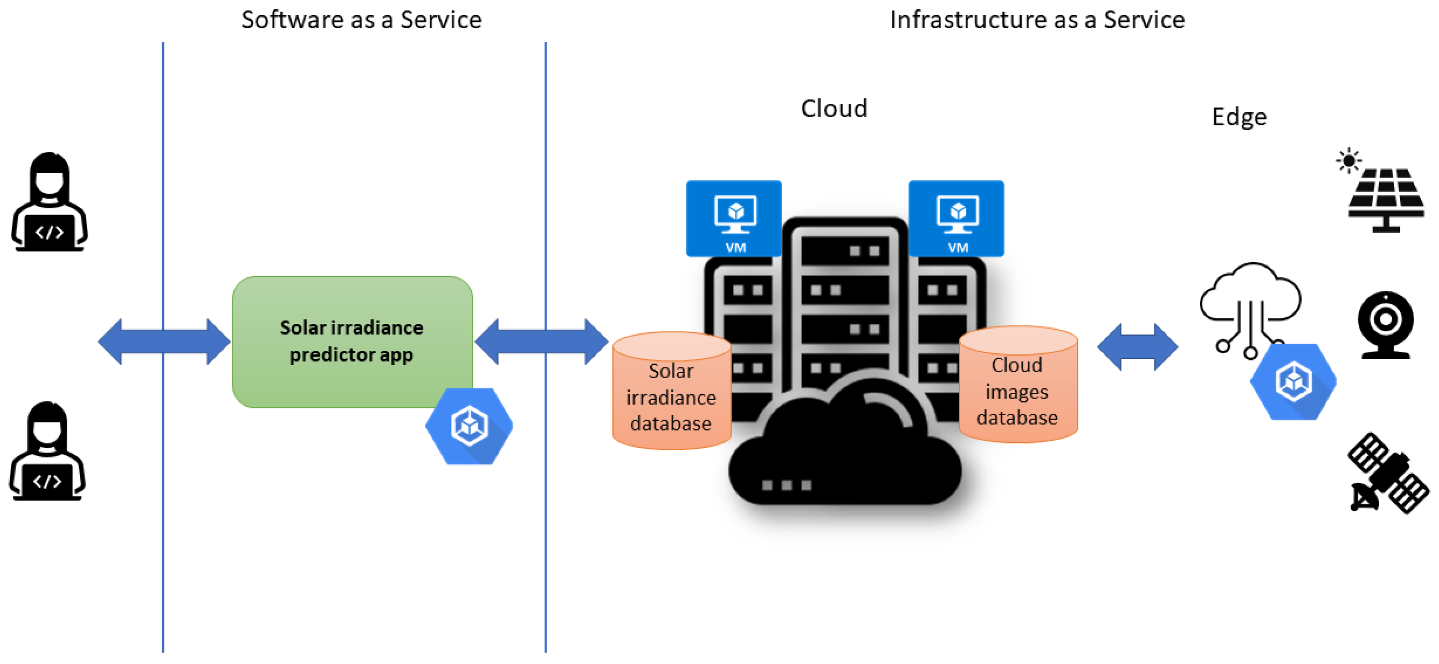
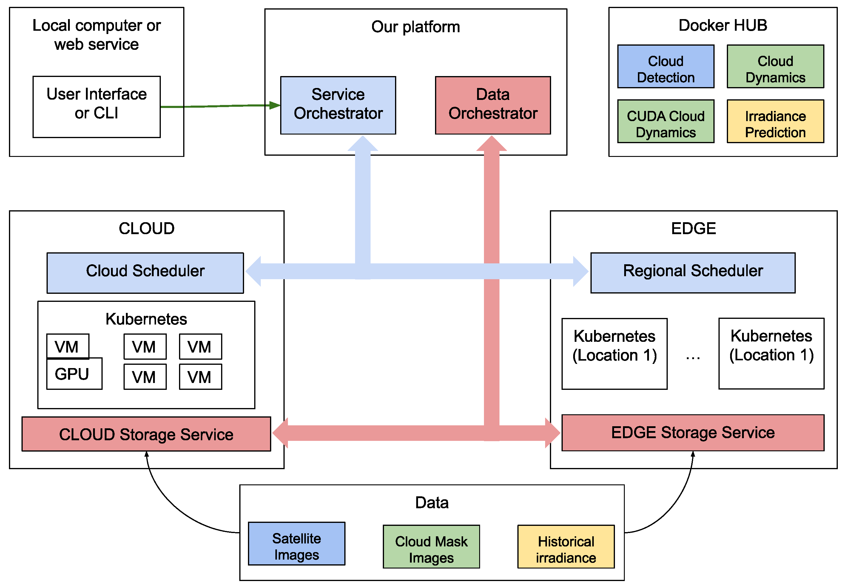
3. Proposed Architecture

The last decade has seen a surge in the computational capabilities of devices lying at the edge of the network. Previously, the computational power was concentrated in big data centres, possessing high bandwidth and inter-connectivity. With the advent of IoT and the prospect of smart technologies, research and industry alike are investing money and effort in designing more capable edge devices, high bandwidth connections, and platforms that will handle the data processing workflows on the cloud–edge continuum. Figure 1 shows our vision of such a layered architecture targeting solar irradiance predictions.

Figure 1. Our vision of a layered architecture spanning the cloud–edge continuum.

Kubernetes [37] is a popular resource management platform, allowing users to scale and automate container applications. The majority of Cloud providers offering container deployments also offer the possibility to create Kubernetes clusters to manage application elasticity. Recently, a lightweight (https://k3s.io/, accessed on 22 August 2022) version of the Kubernetes platform was designed for IoT devices. A preliminary study [38] has shown it has a great advantage with respect to disk, memory, and CPU utilization, as well as time required for different procedures (e.g., add worker, start deployment).

Our proposed architecture enabling hybrid cloud–edge deployment is presented in Figure 2 and consists of several components. The end-user interested in solar radiation prediction will interact with our SaaS solution through a web user interface. Similarly, programmers can access the platform through a REST API. Users will select a geographical region of interest, a prediction window, and the type of data to use. The core of our platform consists of two components: service and data orchestrators. The Service Orchestrator interprets the user request and identifies a set of operations to be carried out. The platform maintains descriptions for the offered services. A service (deployed as a container) is described by some requirements (CPU, memory, GPU), the input/output data types, and a Docker Image (initially stored on Docker Hub, but cached by nodes running the images). Examples of services include our core modules: Cloud Dynamics forecast CPU/GPU enabled, Cloud Detection, and Irradiance prediction.

Figure 2. Detailed architecture of the proposed platform.

The Data Orchestrator component maintains a record of data locations. In the beginning, the data locations are initiated with public data servers containing satellite images and irradiance historical data. As services run and data are transferred, the system will prefer to run subsequent applications near the new location for the data.

The Service Orchestrator uses the data location information to select a set of services that need to be run to achieve the desired result. For example, if cloud masks have been generated by a previous user request and have been stored in a storage bucket or FTP server, then the Cloud Detection/Dynamics services do not need to be executed again. Moreover, if cloud masks have already been predicted for a region and they are still valid (i.e., the interval where the accuracy of the model is under a predetermined threshold) they can be reused by the irradiance prediction service. In general, this component will create a workflow consisting of a Directed Acyclic Graph (DAG) where nodes represent the services and edges represent data dependencies between services.

The Service Orchestrator will ask one or more Cloud and Edge Scheduling components to find resources for running the services, providing back a solution. For the Cloud Dynamics service, our platform offers two implementations: a CPU and a GPU version. In this case, the GPU version will be preferred. If there are no free GPUs for the scheduler, then a workflow with the CPU version is requested.

A Cloud Scheduler manages a Kubernetes cluster within a cloud region. A Regional Scheduler manages one or more Kubernetes clusters that are close from a network point of view. The Service Orchestrator has knowledge of multiple Regional and Cloud schedulers from which it can choose the best deployment for a workflow.

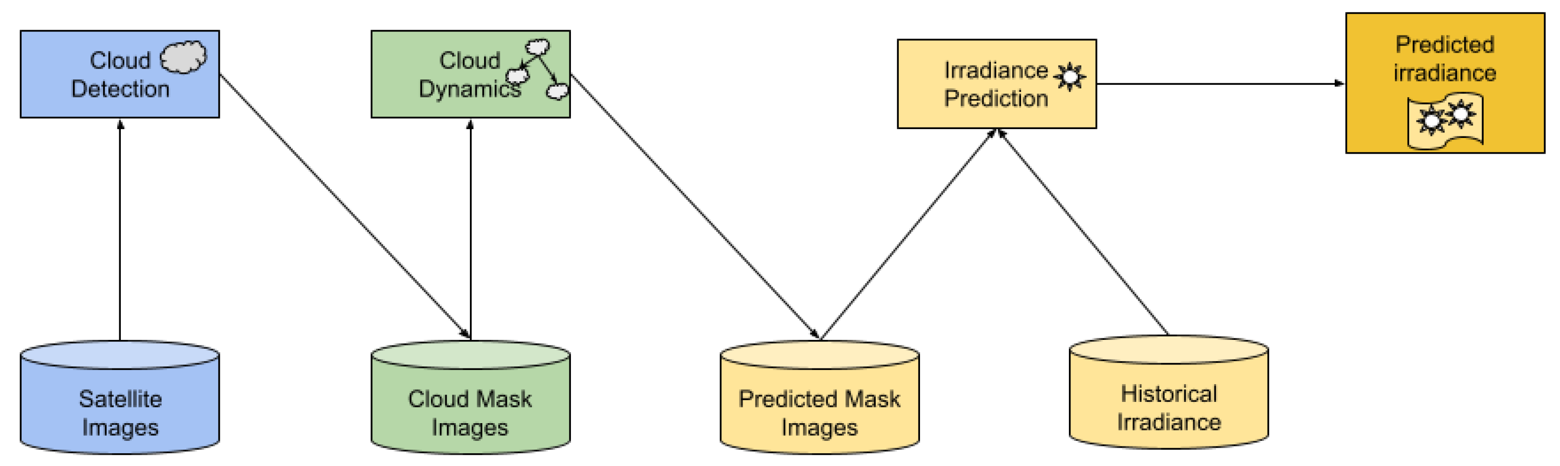
3.1. Example Workflow

In this example, we consider the system in its initial state, with no service or data transfer history. When the first user requests an irradiance prediction for a geographical region, the workflow presented in Figure 3 will be generated by the Service Orchestrator service. First, satellite images need to be made available to the Cloud Detection service using a storage service. This service will generate cloud masks from the recent satellite images. The cloud masks will be used by the Cloud Dynamics service to compute the optical flow and predict the motion of the identified clouds. This will create new cloud masks representing where the clouds will appear in the future. Finally, the Irradiance Prediction service will use the predicted cloud masks and historical irradiance data to forecast the new values.

Figure 3. Full workflow for a prediction.

The cloud mask data will be persisted in Cloud Storage buckets to be reused by subsequent runs of the Cloud Dynamics Service. Predicted cloud masks are also cached given that they are valid; when the satellite image database is updated, a new mask has to be generated to replace the predicted one. Finally, predicted irradiance will also be stored short-term, similar to predicted cloud masks.

We assume that generic users are interested in small regions under 100 ${\mathrm{m}}^2$. While the Irradiance Prediction service can work with data relevant for this small region, the Cloud Dynamics service requires a larger area to increase the accuracy of the predicted motion. Therefore, cloud masks can be generated for larger areas (i.e., countries, continents) and used by multiple irradiance prediction services, each interested in a smaller area contained within the cloud mask.

In order to provide the functionalities described in Section 3, the scheduler needs to be aware not only of the state of the data, but also of the hardware features and availability of each node. A service may depend on or prefer several features such as number of cores, amount of memory, disk space, or GPU cards.

Computing nodes must be selected so as to minimize data movement for the entire workflow of the application. In our approach we deploy the services as close to the data as possible. However, nodes in a Kubernetes cluster will use data from a location which may be external to the node, mounted using a network file system. Therefore, all nodes being part of the same cluster are equal from the data locality point of view.

A prediction job involves the setting of several parameters, defined in Table 1. Cloud movement predictions work best for GOES-R images which are captured twice per hour. Using at least 100,000 particles the predictions for cloud movement show an F1-score in the interval of $[0.75,0.4]$ for the first 5 h. More details on the impact of these parameters are presented in [11].

Table 1. Parameters for a Prediction Job.

Parameter	Description
dtype	type satellite data to be used for prediction
frames	number of frames-ahead to be predicted
boids	number of boid-objects to be used for the simulation of cloud movement

3.2. Datasets

Given the different properties and availability of free data sources the proposed platform supports different formats (e.g., satellite, all-sky camera). Traditional cloud-type inference algorithms rely on multispectral images from satellites, but short-term forecasts usually employ all-sky RGB cameras as multispectral images at such a frequency are usually not freely available. In Table 2 we have listed the characteristics of each Sentinel 2 band and the closest wavelength-wise correspondents from Meteosat SEVIRI and NOAA GOES-R. Ideally, each module will process the same dataset, but some data benefit a module more than the other.

Table 2. Sentinel 2 vs. Meteosat SEVIRI vs. NOAA GOES (closest correspondence bands).

			Sentinel	Meteosat	NOAA
Band	Resolution	Wavelength	Purpose	SEVIRI	GOES-R
1	60 m	443 nm	Aerosol detection	n/a	n/a
2	10 m	490 nm	Color Blue	n/a	Band 1
3	10 m	560 nm	Color Green	n/a	n/a
4	10 m	665 nm	Color Red	Band 1 VIS0.6	Band 2
5	20 m	705 nm	Vegetation	n/a	n/a
6	20 m	740 nm	Vegetation	n/a	n/a
7	20 m	783 nm	Vegetation	Band 2 VIS0.8	n/a
8	10 m	842 nm	Near Infrared	Band 2 VIS0.8	Band 3
8A	20 m	865 nm	Vegetation	n/a	Band 3
9	60 m	945 nm	Water Vapor	n/a	n/a
10	60 m	1375 nm	Cirrus Cloud	n/a	Band 4
11	20 m	1610 nm	Snow-Ice-Cloud	Band 3 NIR1.6	Band 5
12	20 m	2190 nm	Snow-Ice-Cloud	n/a	Band 6

The Cloud Dynamics module was tested and works best on images from geostationary satellites because they are locked to the rotation of the Earth and capture images every 15 min to 30 min. The images from these satellites are especially suitable for detecting cloud movement and forecasting cloud position. The downside, however, is that rotation-locked satellites operate at very high altitudes and the produced images have low spatial resolutions, negatively impacting the forecast precision in terms of extent. Results are good for large regions, but they are not granular enough to be useful on lower scales such as street- or neighborhood-wide forecasts. In addition, freely available datasets are not multispectral rendering them unsuitable for inferring cloud types (Section 3.4).

The Cloud (type) Detection module was tested on images from the orbiting Sentinel 2 satellite. Its onboard sensors have a higher spatial resolution (approx. 10 m/pixel) enabling precise isolation of cloudy pixels from land and water. Clouds can be separated by type and ground-measured irradiance data can be correlated with clouds that are directly on top of the irradiance sensor. Not being locked to the rotation of the Earth means that Sentinel has its orbit and is much closer to the ground than geostationary satellites. The downside is that it takes 2–3 days for the satellite to pass over the same geographic region, so there is a trade-off between higher resolution images and higher frequency captures: one is good for precise detection of cloud types and correlating with irradiance at large intervals, the other is better for forecasting cloud dynamics.

For testing this module we used the following datasets:

• Imagery from NOAA Goes satellite. The color composite images from this geostationary satellite include North America and are captured at 30 $\min$ intervals. The dynamics module was tested on 1920 × 1080 pixel images from 2017 onward.
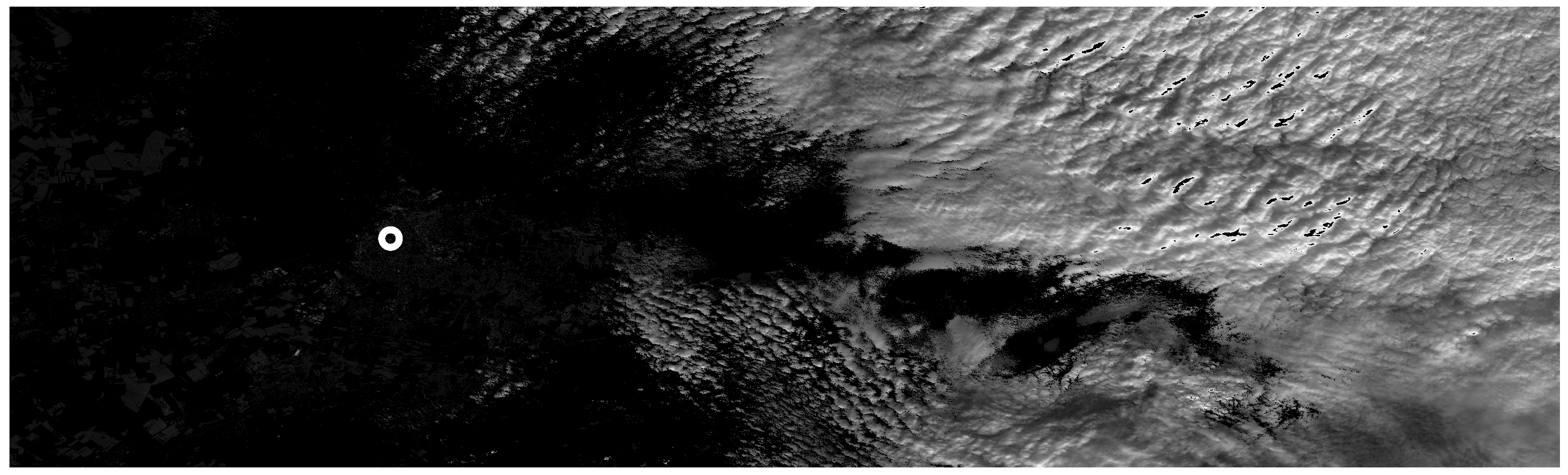
• Imagery from Sentinel 2. The orbiting satellites provide imagery in 13 reflectivity bands (see Table 2) at 10, 20, and 60 m spatial resolutions. We used imagery that captured western Romania, which includes the city of Timisoara where the solar platform providing our irradiance data is installed. Images were retrieved for the years 2020 and 2021. Sentinel images are squares with a width of 10,980 pixels.
• Irradiance from a solar platform. The West University of Timisoara (UVT) has a solar radiation station that measures irradiance among other metrics. We retrieved GI and DI in days where Sentinel imagery was also available.

The modules were tested on different datasets due to the trade-off between time and spatial resolutions. Geostationary satellites have dense temporal resolution, but lack the spatial resolution of low orbit satellites. Next, we detail each module (since they are exposed as services we will use the terms interchangeably).

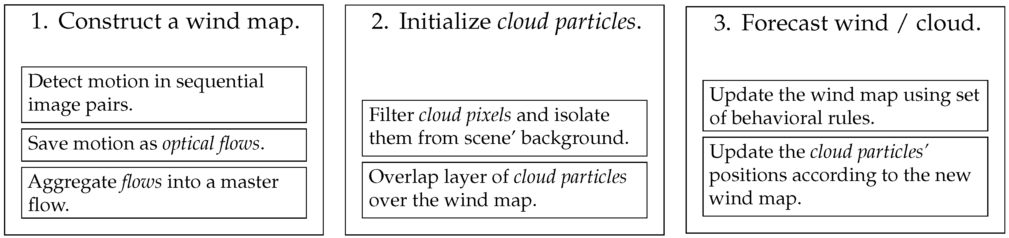
3.3. Cloud Dynamics Module

The module responsible for detecting and forecasting motion uses the optical flow technique proposed by Farnebäck [19] and a modified version of the flocking behavior meta-heuristics developed by Reynolds [39] to simulate the synchronous movement of animal groups. Figure 4 illustrates the three main stages of the cloud motion forecast.

Figure 4. Processing workflow of the Dynamics Module.

The module requires a series of sequential satellite images. It then proceeds by analyzing all sequential pairs using optical flow and generates a master flow from the resulting set of displacement fields [13]. The master flow is an average of the movement detected in the scene, so we consider it to be similar to a wind map of the scene as cloud motion is driven by windand clouds are the only moving object in the scene. Changes caused by humans are not visible. For instance, geostationary weather satellites capture images of the same geographical regions every 15 min to 30 min and surface land or water features are constant. Events such as urbanization or deforestation are visible in larger time scales, so they do not impact the movement detection of clouds.

After the wind map is generated, the service overlaps a layer of “cloud particles” arranged according to a mask of the last known clouds’ position. The mask is initially inferred from the displacement field of the last motion detection, based on the above-mentioned movement arguments. However, the Cloud Detection module can also be used to generate a mask for this step. A benefit of doing so is that we obtain opacity data alongside cloud position. This, in turn, helps for better forecast and cloud form visualization. The cloud particle layer exists in the same space as the wind map, i.e., each particle is positioned directly on top of a motion vector.

Finally, the module applies the modified version of the flocking algorithm on the wind map to simulate movement and forecast cloud position. The algorithm uses rules that update each motion vector in the wind map according to its surroundings and takes into consideration real-world wind behavior. A detailed explanation as well as a discussion on its accuracy is provided in [12]. A motion vector is affected by neighbors that move towards it and will change the direction of motion to match its neighbors’. To mimic wind, motion vectors forming a curved path will be nudged outwards by lessening the turning degree magnitude. The application of the rules to the entire wind map generates a new wind map which then affects the layer of cloud particles by essentially carrying each “cloud particle” according to its corresponding motion vector. The updated cloud particle layer represents the forecast cloud position. Repeated and continuous application of the rules on the wind map and updating of the cloud layer output multiple forecasts that follow each other. The time interval between the forecasts is equal to the image frequency, i.e., 15 min to 30 min.

The proposed model can be applied in the real world with medium to high precision for the first 5 h of forecast (Section 3.1 and Section 4.1, and [11]). Our proposed model is advantageous because it can simulate non-linear cloud particle dynamics. The drawbacks of this model are related to condensation and evaporation, which are not taken into account in the current version.

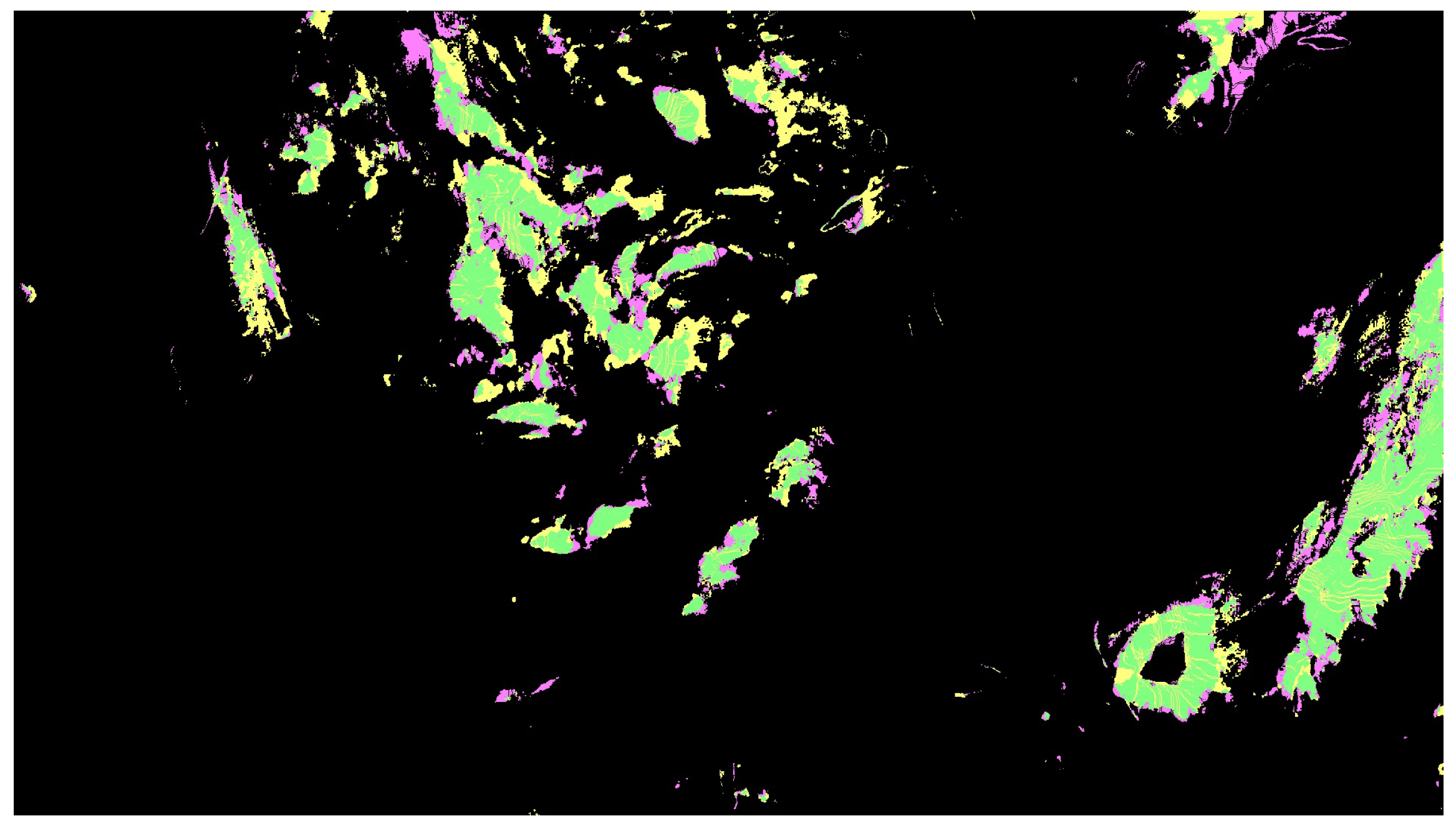
3.4. Cloud Detection Module

Clouds can be detected and their types determined from multispectral images [29]. These are openly available (to a varying degree) both from Earth Observation (EO) satellites (e.g., Sentinel 2) and from geostationary weather satellites (e.g., Meteosat, NOAA GOES). Usually a combination of red, vegetation, and (near) infrared images is used [40], but some satellites have special bands for high-altitude cirrus clouds. The advantage of EO satellites is spatial resolution (reaching as low as a few meters); however, the frequency of images over a given area is unsuited for PV energy output forecast.

For instance, Sentinel 2 captures images of Earth using 13 bands that were built specifically for different types of remote sensing (Table 2), Meteosat SEVIRI has 12 bands [41], and NOAA GOES-R has 16 bands [42].

In what follows we rely on Sentinel 2 naming from Table 2 for clarity. Since it has been shown that thresholding values depend on the region (e.g., water, land, ice) [43] we present next an algorithm working over land as PV farms which interest us are placed on soil.

To identify the types of cloud in an image, we use a thresholding method that combines information from four Sentinel 2 bands: the red band (B04), the near-infrared band (B08), the water vapor band (B09), and the cirrus band (B10). It can be seen that not all these bands are present in geostationary satellites with some offering close approximations. This makes it challenging in using these images to extract cloud types but they can be used for cloud masks as shown in Section 3.3. Before proceeding we note that some cloud types (e.g., cirrus, low stratus, roll cumulus) are difficult to detect because of insufficient contrast with the surface radiance [43]. Our aim is to detect three types of clouds: thick convective clouds (cumulonimbus), low clouds (fog, stratus), and thin high clouds (cirrus). The choice of cloud types is motivated by the published work of Menzel [44], in which he details best practices to identify clouds using multiple wavelength tests. A general algorithm for extracting clouds (from Landsat images) is given in [45] (and adapted by us to Sentinel 2 bands):

$$\mathrm{B}04 > 0.15 \mathtt{and} \mathrm{B}11 > 0.12 \mathtt{and} \mathrm{B}04 > 0.65 ·\mathrm{B}011 \Rightarrow \mathtt{cloud}$$

(1)

where the values for the B* bands indicate the top-of-atmosphere reflectance.

The module first isolates most clouds by performing a reflectance ratio test [43] involving the red (660 nm band—B04) and near-infrared (870 nm band—B08) bands. For each pixel, it computes the ratio between the two bands and tests that it is between 0.9 and 1.1 but could be lowered to as much as 0.8 or 0.75 in some cases:

$$ratio=\mathrm{B}{08}_{ij}/\mathrm{B}{04}_{ij},$$

(2)

$$0.9\le ratio\le 1.1\left\{\begin{array}{cc}\mathtt{true},\hfill & allCloudMask=\mathrm{B}{08}_{ij};\hfill \\ \mathtt{false},\hfill & allCloudMask=0,\hfill \end{array}\right.$$

(3)

where i and j are the pixel’s coordinates, and allCloudMask represents the cloud mask. It is common to use the 865 nm vegetation band (B8A) instead of the 842 nm near infrared band (B08), but the latter has a wider bandwidth of 115 nm versus the former’s 20 nm. This means that the two bands overlap and the near infrared band (B08) captures a wider spectrum than the vegetation band (B8A) which can be considered a subset.

Convective as well as stratiform clouds are detected using the near-infrared (B08) and water vapor (B09) bands (the brightness temperature in the water vapor absorption channel is warmer than that in the atmospheric infrared window [46]):

$$\mathrm{B}{08}_{ij}-\mathrm{B}{09}_{ij}<0\left\{\begin{array}{cc}\mathtt{true},\hfill & convCloudMask=\mathrm{B}{08}_{ij};\hfill \\ \mathtt{false},\hfill & convCloudMask=0,\hfill \end{array}\right.$$

(4)

where convCloudMask represents the convective cloud mask. Difference tests such as this one are often named split windows techniques and usually involve using 11.000 nm wavelengths and over, but Sentinel 2 has its largest band centered around 2190 $\mathrm{n}$$\mathrm{m}$ thus we use different wavelengths to perform the tests.

Recently, an algorithm relying on red and infrared bands was proposed [47].

Low altitude clouds (fog, stratus) are identified by removing convective clouds from the initial cloud mask:

$$difference=allCloudMas{k}_{ij}-convCloudMas{k}_{ij},$$

(5)

$$difference>0\left\{\begin{array}{cc}\mathtt{true},\hfill & lowCloudMas{k}_{ij}=difference;\hfill \\ \mathtt{false},\hfill & lowCloudMas{k}_{ij}=0,\hfill \end{array}\right.$$

(6)

where convCloudMask represents the convective cloud mask.

Another approach is to use B11 band which discriminates low clouds from snow [48].

The cirrus band (B10) in near infrared is specifically designed for detecting high-thin cirrus so the resulting image is directly used as a mask for cirrus clouds.

Masking is performed for all available images in the time series.

3.5. Irradiance Prediction Module

Finally, the irradiance prediction module computes the correlation between the GI and DI, and the values of the masked cloud types. Since determining the cloud type is a rather challenging and inaccurate (Section 2 and Section 3.4) process due to the required parametrization, we also correlate irradiance levels directly with RGB information to verify the predictability of irradiance without a priori knowledge of cloud types as inferring them requires, in most cases, multispectral images not easily accessible by the general public (Section 3.4. Despite having 13 bands, only some of the wavelengths are sensitive to or interfere in any way with clouds. Therefore, we compute correlations only for specific bands (Table 2).

The module receives geographic coordinates for the location of the nearby solar platform (for which we have irradiance data) and then retrieves the pixel values for the point of interest (i.e., the pixel directly above the PV farm and solar station) corresponding to bands 1 through 4, 8 through 12, TCI (True Color Image – auto-generated composite by the Sentinel processing system), and the allCloudMask values identified by the formula at Equation (3). TCI contain all data available in the visible spectrum, not just cloud information. This includes land and water surfaces, buildings, roads, forests, and open fields. For all-sky cameras, TCI can be replaced by RGB/gray images while the individual R, G, B channels can be used instead of the corresponding multispectral bands from EO satellites.

The resulting series of pixel values are appended to the timestamped irradiance levels according to the time of image acquisition (Table 3). The purpose is to have separate columns for irradiance levels and pixel values of each of the studied wavelengths. Each row represents the exact time at which spectral data were captured by the satellite and irradiance levels recorded by the solar platform. Each retrieved cloud mask and band series is correlated with the two irradiance measures for the entire time series. For our dataset, the cloud detection module detected convective and low clouds in the scene, but not over the solar platform’s location (Figure 5).

Table 3. Examples of retrieved pixel values for different bands and cloud type values. mask1 stands for allCloudMask. GI and DI unit: W/m².

Date	GI	DI	TCI	B01	B02	B03	B04	B08	B09	B10	B11	B12	mask1
1 April 2022	517	312	189	3783	3749	3548	3645	4120	2740	1932	3162	2679	-
4 April 2022	651	270	188	3725	3438	3336	3625	4169	3001	1078	4786	4221	-
6 April 2022	785	83	255	2893	3847	4098	4778	4917	1873	1013	4467	3007	4917
9 April 2022	337	324	255	8261	7866	7344	7937	8232	5618	1628	6243	5220	8232
11 April 2022	940	222	79	2529	2515	2286	2108	2098	1347	1014	1719	1422	2098
14 April 2022	849	118	255	2870	3915	3973	4611	5042	2252	1029	4585	3631	5042
16 April 2022	452	399	234	5216	4651	4182	4279	4860	2971	1033	4697	3978	-
19 April 2022	198	184	255	6587	6725	6314	6902	7452	5179	1273	7096	6187	7452
21 April 2022	854	433	128	2955	2882	2705	2797	3257	2123	1460	2389	2000	-
24 April 2022	832	298	216	2916	3489	3594	4022	4544	1897	1031	4311	3444	-
26 April 2022	821	125	255	2947	3833	4102	4673	5070	1903	1023	4616	3314	5070
29 April 2022	976	165	186	4223	3725	3561	3610	4405	2554	1022	4335	3737	-
1 May 2022	874	110	255	2997	3762	4058	4636	5005	2091	1021	4473	3385	5005
4 May 2022	882	140	255	2935	3885	4133	4766	5252	1829	1015	5027	4021	-
6 May 2022	687	494	191	4113	3881	3700	3669	4817	3353	2467	3182	2853	-
14 May 2022	1013	249	255	3180	4542	4907	5545	6088	1942	1017	5538	4300	6088
16 May 2022	845	172	245	3023	3677	3792	4443	4954	1905	1046	4813	3347	-
19 May 2022	940	98	255	3012	4134	4505	5155	5516	2605	1019	5252	4069	5516
21 May 2022	857	453	255	5237	4986	4727	4753	5764	4041	2324	2927	2711	-

Figure 5. Example of a mask of low clouds detected on 1st January 2022 near Timisoara (marked with a circle.

Therefore, the respective masks were not used in our experiments. A moving window of different time spans (rolling correlation) is also employed to observe the correlation coefficient evolution over time. We utilized 7-, 14-, 30-, and 60-day window widths to obtain weekly, bi-weekly, monthly, and bi-monthly trends. Given the 2- to 3-day capture interval of Sentinel 2, these window sizes typically include 2 to 3, 5 to 6, 11 to 13, and 22 to 25 data-points. The chosen sizes are not themselves significant in terms of the number of snapshots, but are rather intended to provide a way of observing trends at various time intervals. Shortening to sub-weekly size would result in windows with a single data point, and increasing the widths would result in correlations approaching closer to the entire dataset.

After computing the Pearson correlation coefficient, the strongest correlated cloud types—bands pairs are then used to determine irradiance.

We trained an ordinary least-squares linear regression model on the time-series. The model was trained using 75% randomly chosen rows from the dataset and tested on the rest. We assessed performance by computing the coefficient of determination of the prediction, the Mean Absolute Error (MAE), and the Root Mean Squared Error (RMSE). These are the most widely utilized performance metrics in the field of irradiance prediction [49] and are defined as:

$$MAE=\frac{1}{n}\sum _{i=1}^n|p_i-t_i|$$

$$RMSE=\frac{1}{n}\sum _{i=1}^n(p_i-t_i)$$

where n is the test data size, p is the predicted irradiance of the regression model, and t is the expected true value, both for each image i.

4. Results

In this section, we present results for the key modules. In particular, we are interested in the scalability of the cloud dynamics module which is computationally expensive and the irradiance prediction module which enables the forecast of the PV output that is related to the received irradiance.

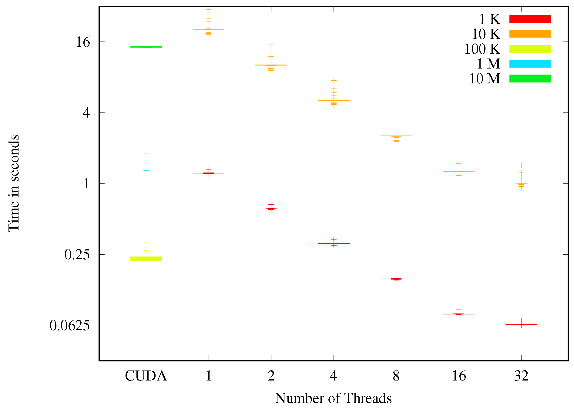
4.1. Scalability and Accuracy of the Cloud Dynamics Module

The particle update function has been implemented to take advantage of GPUs and multicore architectures. We have implemented an OpenMP and CUDA version. The execution time was measured during an experiment with 100 steps, varying the number of particles. For OpenMP, we varied the particle number from 1000 to 10,000 while for the CUDA implementation it varied between 100,000 and 10 million.

Figure 6 accounts for the time spent on copying buffers from and to the device, as well as executing host code that updates particle positions based on the new velocity buffer copied from the GPU. It takes around 0.25 seconds to update the positions for 100,000 particles. We compare this with the time required to simulate the update of 1000 particles using one CPU thread. The speed-up can be computed as $100·\frac{1}{0.25}=400$. The same comparison can be made for 1 million particles achieving a speed-up of 1000. When increasing the size to 10 million particles the performance is degraded due to the amount of single-core host code that updates the particles’ positions, leading to a decrease in speed-up to about 650.

Figure 6. Execution time for predicting one step of cloud movement.

The OpenMP implementation scales well with increasing number of threads, due to the high parallelism of the problem. However, increasing the amount of particles 10-fold causes the processing time to increase 16-fold due to the higher chance of particles being in the neighborhood of other particles.

We compare our approach with the solution presented in [50]. Our solution is tested for millions of particles, while their simulation only reaches 32,768. Their solution is limited by the shared memory size, while our solution uses global memory. In terms of execution time we reach similar results, yet our solution scales to millions of particles due to the data-parallel modelling of the problem.

The output of the Cloud Dynamics module is of two types: binary cloud masks and cloud density maps. Binary cloud masks predict whether a pixel will be covered by clouds or not. In cloud density maps, each pixel encodes the density of the cloud on the area contained by the pixel (0 representing no cloud and 255 representing full opacity). We have created heatmaps that represent the accuracy of the predicted cloud masks when compared with historical data. The accuracy heatmaps are not required for predicting the solar irradiance, but prove useful when testing adaptations to the cloud motion prediction algorithm. Such a heatmap is presented in Figure 7 and shows the accuracy of predicting the motion of the cloud one hour ahead. False positives can appear if the motion of the cloud is wrongly predicted, but also if the cloud has condensed. False negatives can also represent wrong motion prediction, but they can also represent clouds that have just formed due to evaporation. Experiments have shown that in the first hour the F1-score is around 0.75 dropping to 0.2 after 10 h.

Figure 7. Cloud masks for 1-hour ahead. Heatmap: true positives (green), true negatives (black), false positives (magenta) and false negatives (yellow).

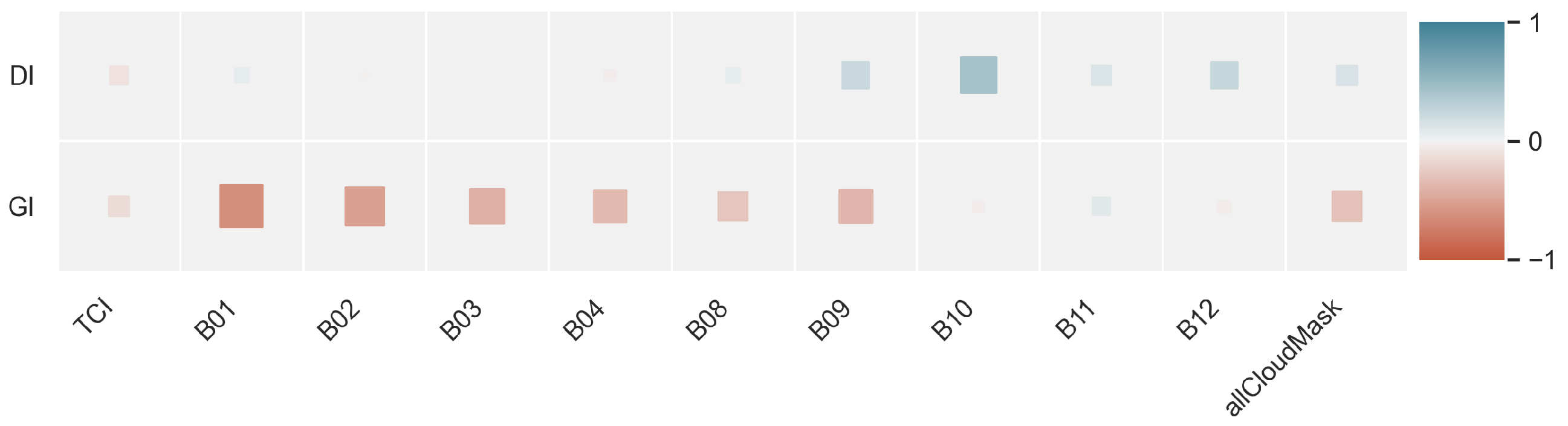
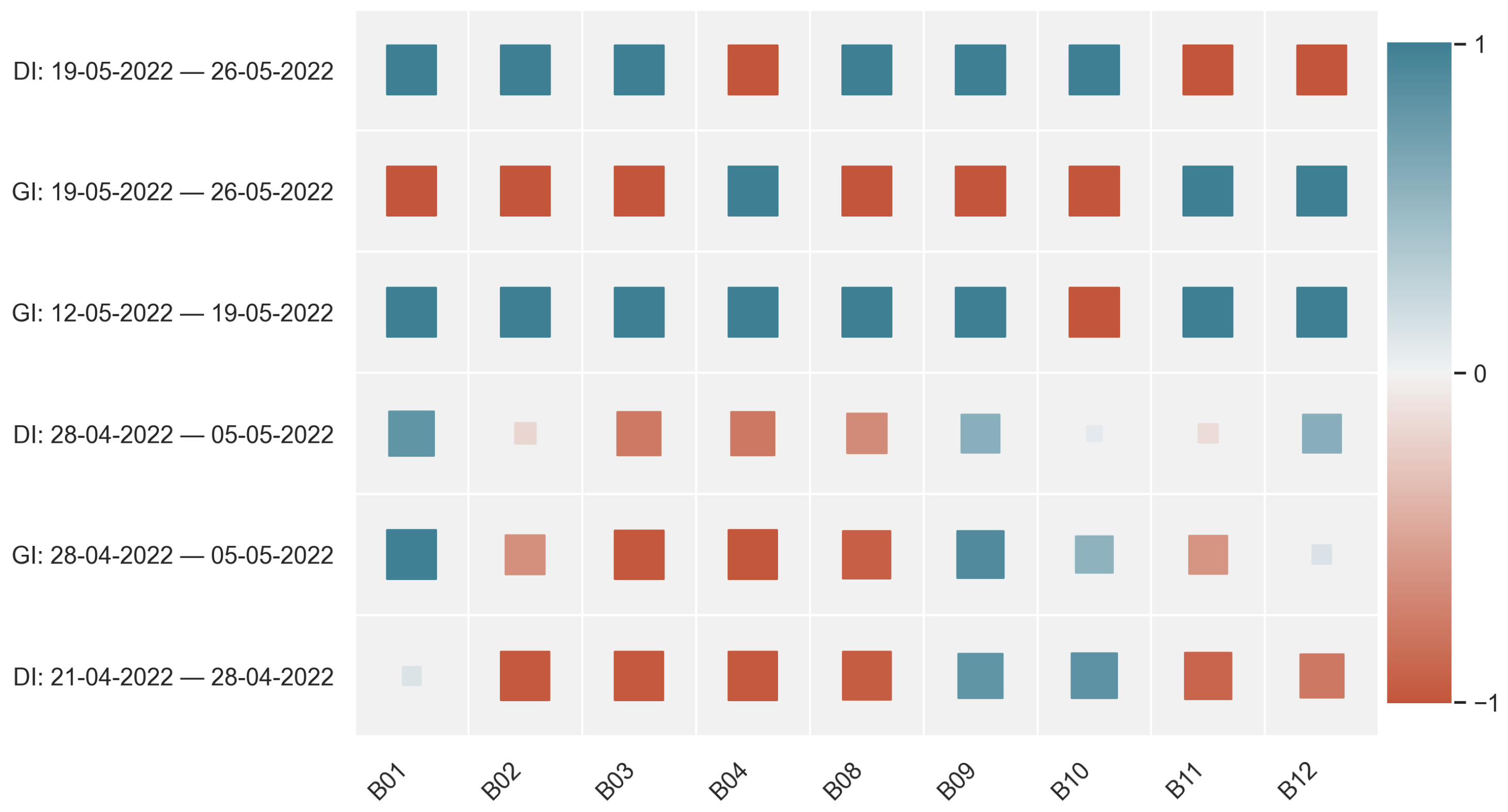
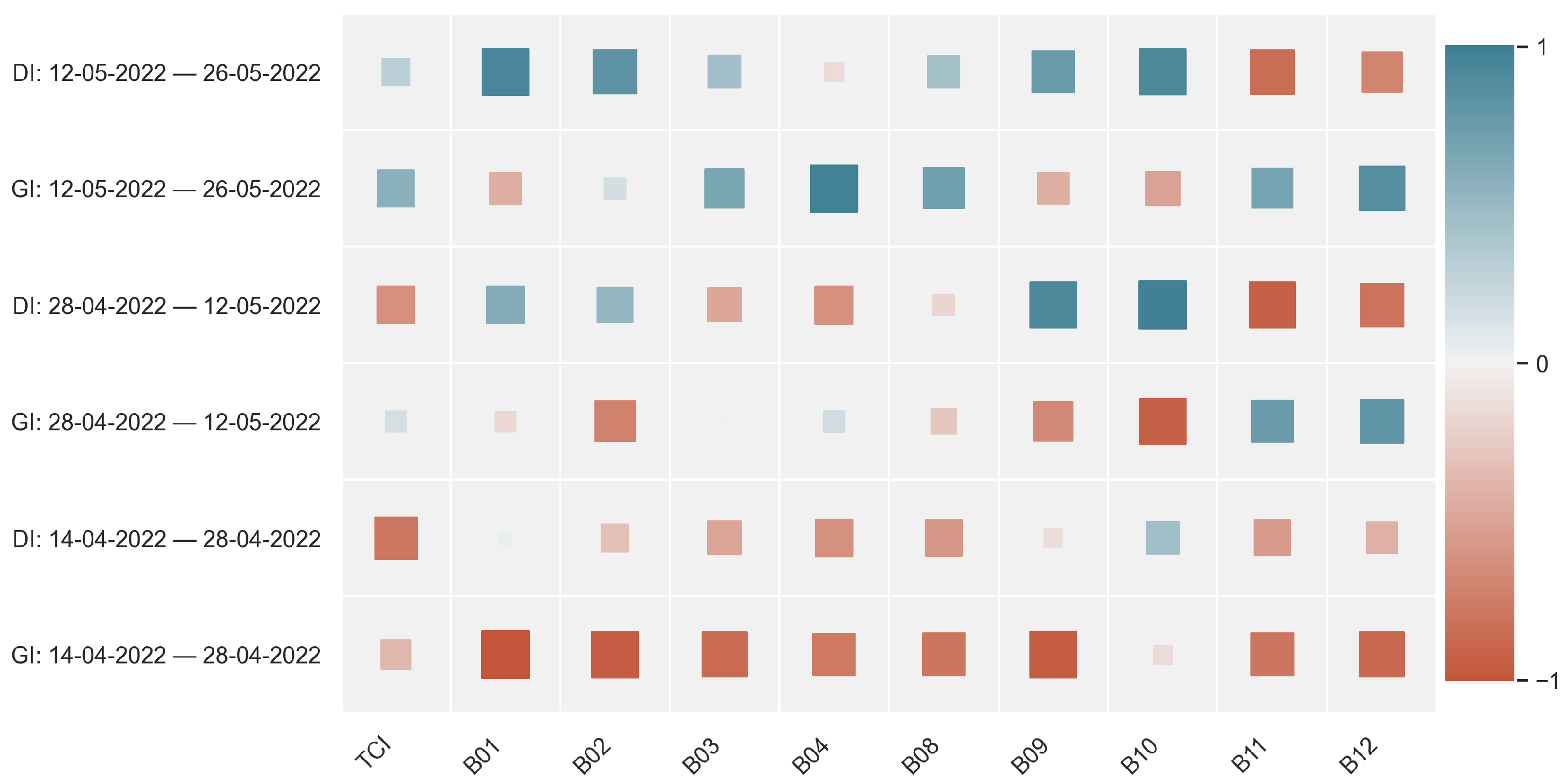
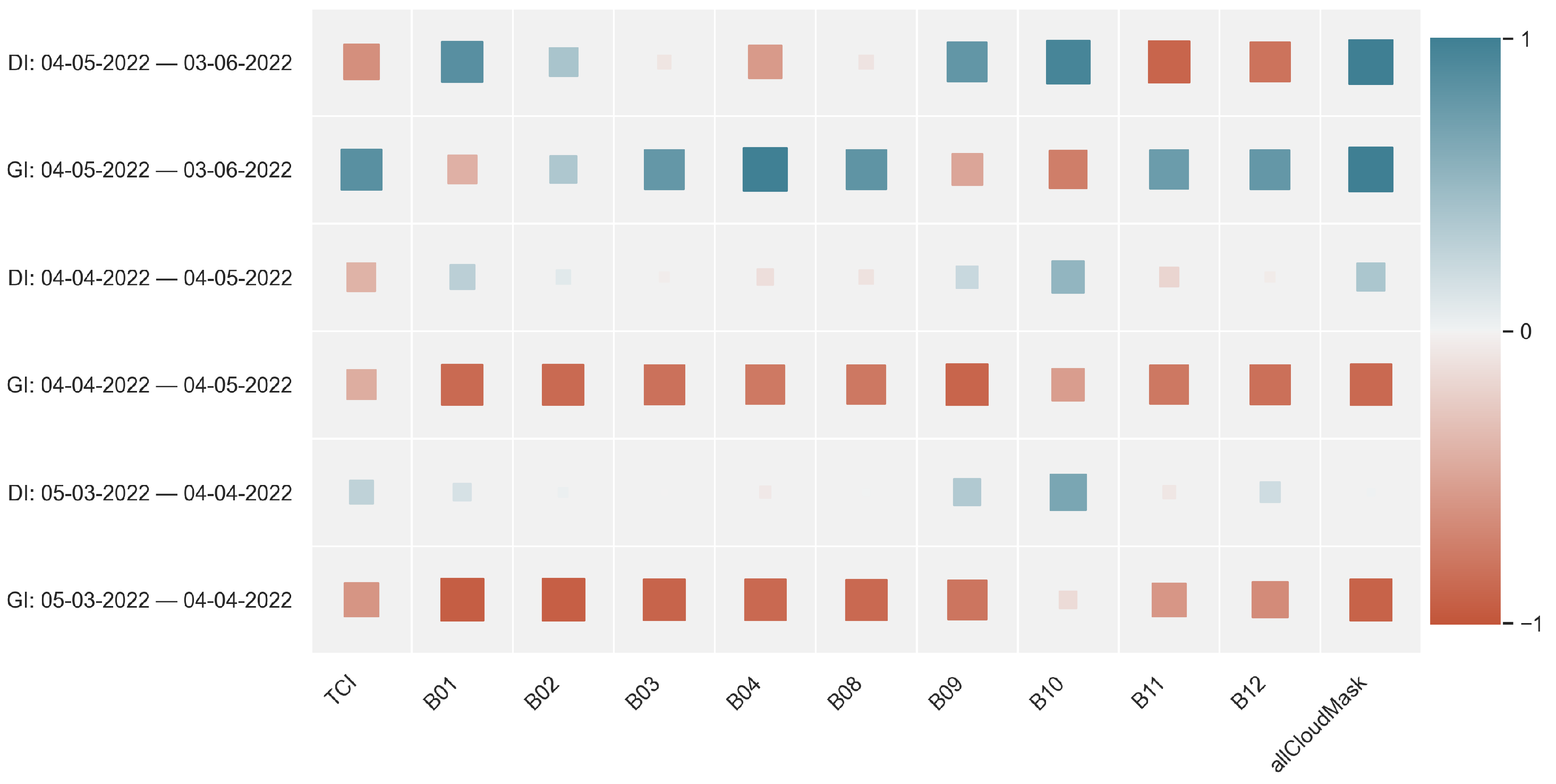
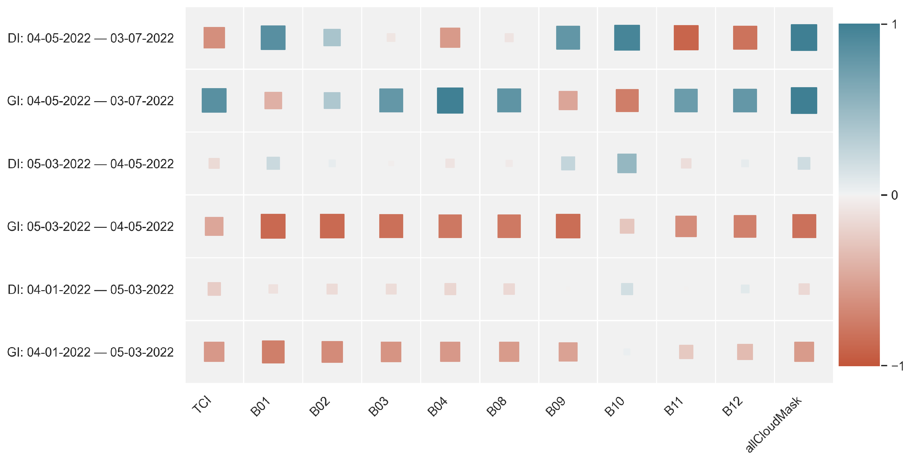
4.2. Correlation Results

We tested for correlation using the Pearson coefficient for DI and GI from the solar platform at the West University of Timisoara, and the retrieved pixel values in Table 2.

The overall correlation of the bands values and the irradiance data is presented in Figure 8. Bands 1, 2, and 3 are most correlated with GI ($-0.6283$, $-0.5078$ and $-0.4041$), and B10 with DI ($0.4188$). The Aerosol band has the strongest coefficient at $-0.6283$ for GI.

Figure 8. Overall correlation between GI, DI, and the Sentinel 2 sensor bands. Opacity and size of the squares reflect correlation intensity: large opaque squares denote strong correlations, and small translucent squares are attributed to weak or not correlated pairs.

Similar tests on smaller dataset windows resulted in stronger coefficients, so we performed rolling correlations to observe short-time relationships over time using non-overlapping fixed window widths. This approach can demonstrate how the bands correlate with the irradiance data chronologically over the weeks and months encompassed by the dataset.

The seven-day window rolling correlation (e.g., Figure 9) resulted in numerous fully correlated weekly windows because, as previously mentioned, a week has either two or three satellite snapshots. Correlations for two data-points result in perfect positive or negative relationships. The side-effect is that although each interval is fully correlated, the coefficients do not reflect longer-term relationships.

Figure 9. Example of 7-day window correlations.

Figure 10, Figure 11 and Figure 12 show sections of rolling correlations for 14-, 30-, and 60-day windows. It is observed that GI is correlated stronger with the spectral bands than DI. This can be intuitively expected as DI represents irradiance reaching the sensor after it has scattered in the atmosphere and not in a direct trajectory from the sun [51]. GI consists of DI components and direct irradiance from above. The most promising values are those from the color bands (2, 3, and 4), WV, and the mask of all clouds (which is stronger than the NIR correlation). The color bands have coefficients between $\pm 0.4$ and $\pm 0.85$ most of the time, but return towards 0 in situations where the image is overcast.

Figure 10. Example of 14-day window correlations.

Figure 11. Example of 30-day window correlations.

Figure 12. Example of 60-day window correlations.

The correlation coefficients approach close to 0 in certain time periods when the satellite snapshots are overcast with numerous bright clouds. Figure 13 shows information for band 4 (red) and the TCI composite for an overcast snapshot captured on 27 December 2021.

Figure 13. Example of a bright overcast scene over Timisoara on 27 December 2021. Band 4 (left) and TCI (right). The TCI image is almost completely white with some spots of darker pixels in the upper left and bottom of the scene.

The entire scene is covered by bright opaque clouds leading to disproportionately increased pixel values (saturated) and weaker correlation coefficients.

Table 4 and Table 5 show the computed error scores of the linear regression model for TCI, each spectral band, and mask1. The best $R^2$ Coefficient for GI prediction was 0.18979 for B04, and the best MAE and RMSE scores were 206.04135 Wm⁻² and 243.33684 Wm⁻² for B10. The best $R^2$ Coefficient for DI prediction was 0.03297 for B12, and the best MAE and RMSE scores were 66.96541 Wm⁻² and 91.83242 Wm⁻² for mask1. The obtained scores are better than naive persistence’s 173.83 Wm⁻² MAE [49] and comparable to other solar irradiance prediction methods [51,52] reaching between 58.75 Wm⁻² to 395.12 Wm⁻² MAE, and between 84.86 Wm⁻² to 462.93 Wm⁻² RMSE.

Table 4. $R^2$ Coefficient, MAE, and RMSE for predicting GI. Best scores are highlighted in bold.

	${\mathit{R}}^2$ Coefficient	MAE	RMSE
TCI	0.03644642678338772	242.42154794617383	274.7408497562563
B01	0.0820348043032918	230.80298574638536	262.10447565483634
B02	−0.21622423375748578	226.0133833016301	266.59864257524436
B03	0.16484461491503566	258.6680008229855	289.54645358512585
B04	0.18979026867512105	242.25312734146155	278.8299007436962
B08	−0.004685782814821238	263.14349948394886	297.98935481964486
B09	0.1666511708442644	213.59486036305327	243.97853837735866
B10	−0.014280286109260798	206.04134647422316	243.33683919725743
B11	−0.09136205237619488	213.875380476756	253.2442376883533
B12	−0.015120462726200268	275.1958711048938	311.08537403125933
mask1	−0.03157307096771955	261.67319967290194	317.8092308395099

Table 5. $R^2$ Coefficient, MAE, and RMSE for predicting DI. Best scores are highlighted in bold.

	${\mathit{R}}^2$ Coefficient	MAE	RMSE
TCI	−0.0994881915821475	109.1422687328849	139.87949383832782
B01	−0.04660898451208051	91.47501179095161	125.09773057981627
B02	−0.006483852227510134	87.28399557078228	112.28440557826498
B03	−0.03451064554614436	90.44762037974252	107.51985827433974
B04	−0.019033305619853502	81.80569395778589	101.4159979735758
B08	−0.024606201009772732	75.72686996307678	97.97877522070938
B09	−0.11615994107608651	100.78955376918246	134.09884693197583
B10	0.017187645831838072	81.23618926107555	114.61636948767924
B11	−0.05413538201239265	96.29763294968915	126.01369289709537
B12	0.03296695291836593	82.92904576107716	108.01263505006585
mask1	−0.04226888637819548	66.96540604389577	91.83241938981622

5. Conclusions

Predicting PV output is a challenging task due to the complexity of numerical models and access to near real-time satellite images. In this paper, we propose a hybrid edge–cloud platform that leverages the new multi- and many-core commodity platforms near the PV farm (edge) with the high availability and processing power of cloud systems. In addition to assessing the efficiency of processing data near the edge via scalability tests, we investigated the possibility of inferring irradiance directly from the pixel values, bypassing in the process the non-trivial cloud type identification step. Despite access to a large open database and irradiance values from the UVT solar station, we could identify only one cloud type over the location of the solar platform further supporting our alternative solution. Other types (e.g., low and convective) were detected but not at the solar platform position. Results showed that individual bands such as the aerosol, blue and green bands, and the mask of all clouds are strongly correlated with GI most of the time. The overall correlations for bands 1 through 4 with GI are $-0.6283$, $-0.5098$, $-0.4055$, and $-0.3492$. The strongest correlated with DI is band 10 at $0.4304$. Rolling correlations show that coefficients are stronger for window widths that do not include bright overcast images. These results indicate that for GI it is possible to use the negative correlation to infer values from the pixel value. Further experiments with a larger dataset are needed in the case of DI.

Future work will investigate the suitability of using powerful near edge devices such as NVIDIA Jetson boards to group resources at the aggregated fog level, grouping the processing of nearby PV farms’ data together. It will also focus on analyzing the suitability of all-sky camera imagery to be used instead of satellite images.

In addition, we plan to investigate whether the correlation between DI and the same spectral information based on an average value of pixel data around the solar station region is improved compared to the current approach of using just the pixel over it.

Finally, since images and data can contain noise we will further investigate its impact on the accuracy of our results.

References

1. The International Energy Agency. Available online: https://www.iea.org/reports/solar-pv (accessed on 15 November 2021).
2. Fara, L.; Diaconu, L.; Craciunescu, D.; Fara, S. Forecasting of Energy Production for Photovoltaic Systems Based on ARIMA and ANN Advanced Models. Int. J. Photoenergy 2021, 2021, 677488. [Google Scholar] [CrossRef]
3. Fabbri, A.; Roman, T.; Abbad, J.; Quezada, V. Assessment of the cost associated with wind generation prediction errors in a liberalized electricity market. IEEE Trans. Power Syst. 2005, 20, 1440–1446. [Google Scholar] [CrossRef]
4. Clouds and Solar Radiation-Remote Sensing of the Ocean and Atmosphere Atmosphere. Available online: https://marine.rutgers.edu/dmcs/ms552/f2008/solar_cloud.pdf (accessed on 15 November 2021).
5. Valk, P.; Feijt, A.; Roozekrans, H.; Roebeling, H.; Rosema, A. Operationalisation of an Algorithm for the Automatic Detection and Characterisation of Clouds in METEOSAT Imagery; Technical Report; BCRS Report 1998: USP-2: NRSP-2: NUSP; Beleidscommissie Remote Sensing (BCRS): Delft, The Netherlands, 1998. [Google Scholar]
6. Zamo, M.; Mestre, O.; Arbogast, P.; Pannekoucke, O. A benchmark of statistical regression methods for short-term forecasting of photovoltaic electricity production, part I: Deterministic forecast of hourly production. Solar Energy 2014, 105, 792–803. [Google Scholar] [CrossRef]
7. IEA. Regional Solar Power Forecasting; Technical Report, IEA. 2020. Available online: https://iea-pvps.org/key-topics/regional-solar-power-forecasting-2020/ (accessed on 15 November 2021).
8. Kleissl, J. Solar Energy Forecasting and Resource Assessment; Academic Press: Boston, MA, USA, 2013. [Google Scholar] [CrossRef]
9. Validation of short and medium term operational solar radiation forecasts in the US. Solar Energy 2010, 84, 2161–2172. [CrossRef]
10. Oana, L.; Frincu, M. Benchmarking the WRF Model on Bluegene/P, Cluster, and Cloud Platforms and Accelerating Model Setup Through Parallel Genetic Algorithms. In Proceedings of the 2017 16th International Symposium on Parallel and Distributed Computing (ISPDC), Innsbruck, Austria, 3–6 July 2017; pp. 78–84. [Google Scholar] [CrossRef]
11. Spataru, A.; Tranca, L.C.; Penteliuc, M.E.; Frincu, M. Parallel Cloud Movement Forecasting based on a Modified Boids Flocking Algorithm. In Proceedings of the 2021 20th International Symposium on Parallel and Distributed Computing (ISPDC), Cluj-Napoca, Romania, 28–30 July 2021; pp. 89–96. [Google Scholar] [CrossRef]
12. Penteliuc, M.E.; Frincu, M. Short Term Cloud Motion Forecast based on Boid’s Algorithm for use in PV Output Prediction. In Proceedings of the 2021 IEEE/PES Innovative Smart Grid Technologies Europe (iSGT Europe, Espoo, Finland, 18–21 October 2021. [Google Scholar]
13. Penteliuc, M.; Frincu, M. Prediction of Cloud Movement from Satellite Images Using Neural Networks. In Proceedings of the 2019 21st International Symposium on Symbolic and Numeric Algorithms for Scientific Computing (SYNASC), Timisoara, Romania, 4–7 September 2019; pp. 222–229. [Google Scholar] [CrossRef]
14. SolCast. 2019. Available online: https://solcast.com (accessed on 27 November 2021).
15. Solar Forecasting Accuracy Improves by 33% through AI Machine Learning. 2019. Available online: https://www.solarpowerportal.co.uk/news/solar_forecasting_accuracy_improves_by_33_through_ai_machine_learning (accessed on 27 November 2021).
16. Meniscus Solar Map—Solar Irradiance Predictions for the Next 2 1/2 Hours. Available online: www.meniscus.co.uk/solutions-built-using-meniscus-analytics-platforms/map-solar-predicts-solar-irradiance/ (accessed on 27 November 2021).
17. Hamill, T.M.; Nehrkorn, T. A short-term cloud forecast scheme using cross correlations. Weather. Forecast. 1993, 8, 401–411. [Google Scholar] [CrossRef]
18. Panofsky, H.A.; Brier, G.W. Some Applications of Statistics to Meteorology; Mineral Industries Extension Services, College of Mineral Industries: State College, PA, USA, 1958. [Google Scholar]
19. Farnebäck, G. Two-Frame Motion Estimation Based on Polynomial Expansion. Image Analysis; Bigun, J., Gustavsson, T., Eds.; Springer: Berlin Heidelberg: Berlin/Heidelberg, Germany, 2003; pp. 363–370. [Google Scholar] [CrossRef] [Green Version]
20. Chow, C.W.; Belongie, S.; Kleissl, J. Cloud motion and stability estimation for intra-hour solar forecasting. Solar Energy 2015, 115, 645–655. [Google Scholar] [CrossRef]
21. Espinosa-Gavira, M.J.; Agüera-Pérez, A.; Palomares-Salas, J.C.; de-la Rosa, J.J.G.; Sierra-Fernández, J.M.; Florencias-Oliveros, O. Cloud motion estimation from small-scale irradiance sensor networks: General analysis and proposal of a new method. Solar Energy 2020, 202, 276–293. [Google Scholar] [CrossRef]
22. Bosch, J.; Kleissl, J. Cloud motion vectors from a network of ground sensors in a solar power plant. Solar Energy 2013, 95, 13–20. [Google Scholar] [CrossRef]
23. Escrig, H.; Batlles, F.; Alonso, J.; Baena, F.; Bosch, J.; Salbidegoitia, I.; Burgaleta, J. Cloud detection, classification and motion estimation using geostationary satellite imagery for cloud cover forecast. Energy 2013, 55, 853–859. [Google Scholar] [CrossRef]
24. Jamaly, M.; Kleissl, J. Spatiotemporal interpolation and forecast of irradiance data using Kriging. Solar Energy 2017, 158, 407–423. [Google Scholar] [CrossRef]
25. Martínez-Chico, M.; Batlles, F.; Bosch, J. Cloud classification in a mediterranean location using radiation data and sky images. Energy 2011, 36, 4055–4062. [Google Scholar] [CrossRef]
26. Goodwin, N.; Collett, L.; Denham, R.; Flood, N.; Tindall, D. Cloud and cloud shadow screening across Queensland, Australia: An automated method for Landsat TM/ETM + time series. Remote. Sens. Environ. 2013, 134, 50–65. [Google Scholar] [CrossRef]
27. Miller, S.D.; Rogers, M.A.; Haynes, J.M.; Sengupta, M.; Heidinger, A.K. Short-term solar irradiance forecasting via satellite/model coupling. Solar Energy 2018, 168, 102–117. [Google Scholar] [CrossRef]
28. Cheng, H.Y.; Yu, C.C. Multi-model solar irradiance prediction based on automatic cloud classification. Energy 2015, 91, 579–587. [Google Scholar] [CrossRef]
29. Mecikalski, J.; Minnis, P.; Palikonda, R. Use of satellite derived cloud properties to quantify growing cumulus beneath cirrus clouds. Atmos. Res. 2013, 120–121, 192–201. [Google Scholar] [CrossRef]
30. Kim, K.H.; Baltazar, J.C.; Haberl, J.S. Evaluation of Meteorological Base Models for Estimating Hourly Global Solar Radiation in Texas. Energy Procedia 2014, 57, 1189–1198. [Google Scholar] [CrossRef]
31. Muneer, T.; Gul, M. Evaluation of sunshine and cloud cover based models for generating solar radiation data. Energy Convers. Manag. 2000, 41, 461–482. [Google Scholar] [CrossRef]
32. Huang, J. ASHRAE Research Project 1477-RP Development of 3012 Typical Year Weather Files for International Locations; Final Report; White Box Technologies: Salt Lake City, UT, USA, 2011. [Google Scholar]
33. Martin, L.; Zarzalejo, L.F.; Polo, J.; Navarro, A.; Marchante, R.; Cony, M. Prediction of global solar irradiance based on time series analysis: Application to solar thermal power plants energy production planning. Solar Energy 2010, 84, 1772–1781. [Google Scholar] [CrossRef]
34. Fu, C.L.; Cheng, H.Y. Predicting solar irradiance with all-sky image features via regression. Solar Energy 2013, 97, 537–550. [Google Scholar] [CrossRef]
35. Cheng, H.Y.; Yu, C.C.; Lin, S.J. Bi-model short-term solar irradiance prediction using support vector regressors. Energy 2014, 70, 121–127. [Google Scholar] [CrossRef]
36. Alzahrani, A.; Shamsi, P.; Dagli, C.; Ferdowsi, M. Solar Irradiance Forecasting Using Deep Neural Networks. Procedia Comput. Sci. 2017, 114, 304–313. [Google Scholar] [CrossRef]
37. Burns, B.; Grant, B.; Oppenheimer, D.; Brewer, E.; Wilkes, J. Borg, Omega, and Kubernetes. Queue 2016, 14, 10:70–10:93. [Google Scholar] [CrossRef]
38. Böhm, S.; Wirtz, G. Profiling Lightweight Container Platforms: MicroK8s and K3s in Comparison to Kubernetes. In ZEUS; Distributed Systems Group, University of Bamberg: Bamberg, Germany, 2021; pp. 65–73. [Google Scholar]
39. Reynolds, C.W. Flocks, Herds and Schools: A Distributed Behavioral Model. In Proceedings of the 14th Annual Conference on Computer Graphics and Interactive Techniques, SIGGRAPH’87, Anaheim, CA, USA, 27–31 July 1987; Association for Computing Machinery: New York, NY, USA, 1987; pp. 25–34. [Google Scholar] [CrossRef]
40. Chapter 2 Cloud Type Identification by Satellites. In Analysis and Use of Meteorological Satellite Images. 2002. Available online: http://rammb.cira.colostate.edu/wmovl/VRL/Texts/SATELLITE_METEOROLOGY/CHAPTER-2.PDF (accessed on 27 November 2021).
41. Wooster, M.J.; Roberts, G.; Freeborn, P.H.; Xu, W.; Govaerts, Y.; Beeby, R.; He, J.; Lattanzio, A.; Fisher, D.; Mullen, R. LSA SAF Meteosat FRP products—Part 1: Algorithms, product contents, and analysis. Atmos. Chem. Phys. 2015, 15, 13217–13239. [Google Scholar] [CrossRef]
42. ABI Bands Quick Information Guides. Available online: https://www.goes-r.gov/mission/ABI-bands-quick-info.html (accessed on 27 November 2021).
43. Menzel, P. Chapter 6 Clouds. In Applications with Meteorological Satellites; WMO Library: Genève, Switzerland, 2001. [Google Scholar]
44. Menzel, W. Remote Sensing Applications with Meteorological Satellites, NOAA Satellite and Information Service; University of Wisconsin: Madison, WI, USA, 2006. [Google Scholar]
45. Oreopoulos, L.; Wilson, M.J.; Várnai, T. Implementation on Landsat Data of a Simple Cloud-Mask Algorithm Developed for MODIS Land Bands. IEEE Geosci. Remote. Sens. Lett. 2011, 8, 597–601. [Google Scholar] [CrossRef] [Green Version]
46. Ai, Y.; Li, J.; Shi, W.; Schmit, T.J.; Cao, C.; Li, W. Deep convective cloud characterizations from both broadband imager and hyperspectral infrared sounder measurements. J. Geophys. Res. Atmos. 2017, 122, 1700–1712. [Google Scholar] [CrossRef]
47. Lee, Y.; Kummerow, C.D.; Zupanski, M. A simplified method for the detection of convection using high-resolution imagery from GOES-16. Atmos. Meas. Tech. 2021, 14, 3755–3771. [Google Scholar] [CrossRef]
48. EUMeTrain: Fog and Stratus. Available online: http://www.eumetrain.org/satmanu/CMs/FgStr/navmenu.php (accessed on 27 November 2021).
49. Nielsen, A.H.; Iosifidis, A.; Karstoft, H. IrradianceNet: Spatiotemporal deep learning model for satellite-derived solar irradiance short-term forecasting. Sol. Energy 2021, 228, 659–669. [Google Scholar] [CrossRef]
50. Husselmann, A.; Hawick, K. Simulating Species Interactions and Complex Emergence in Multiple Flocks of Boids with GPUS. In Proceedings of the IASTED International Conference on Parallel and Distributed Computing and Systems, Innsbruck, Austria, 15–17 February 2011. [Google Scholar] [CrossRef]
51. Li, X.; Ma, L.; Chen, P.; Xu, H.; Xing, Q.; Yan, J.; Lu, S.; Fan, H.; Yang, L.; Cheng, Y. Probabilistic solar irradiance forecasting based on XGBoost. In Proceedings of the ICPE 2021-The 2nd International Conference on Power Engineering, Nanning, China, 9–11 December 2021; pp. 1087–1095. [Google Scholar] [CrossRef]
52. Ramirez-Vergara, J.; Bosman, L.B.; Leon-Salas, W.D.; Wollega, E. Ambient temperature and solar irradiance forecasting prediction horizon sensitivity analysis. Mach. Learn. Appl. 2021, 6, 100128. [Google Scholar] [CrossRef]
Publisher’s Note: MDPI stays neutral with regard to jurisdictional claims in published maps and institutional affiliations.
Article Metrics
Citations
Article Access Statistics
Multiple requests from the same IP address are counted as one view.