Fuzzy Luenberger Observer Design for Nonlinear Flexible Joint Robot Manipulator

Abstract

The process of controlling a Flexible Joint Robot Manipulator (FJRM) requires additional sensors for measuring the state variables of flexible joints. Therefore, taking the elasticity into account adds a lot of complexity as all the additional sensors must be taken into account during the control process. This paper proposes a nonlinear observer that controls FJRM, without requiring equipment sensors for measuring the states. The nonlinear state equations are derived in detail for the FJRM where nonlinearity, of order three, is considered. The Takagi–Sugeno Fuzzy Model (T-SFM) technique is applied to linearize the FJRM system. The Luenberger observer is designed to estimate the unmeasured states using error correction. The developed Luenberger observer showed its ability to control the FJRM by utilizing only the measured signal of the velocity of the motor. Stability analysis is implemented to improve the ability of the designed observer to stabilize the FJRM system. The developed observer is tested by simulation to evaluate the ability of the observer to estimate the unknown states. The results showed that the proposed control algorithm estimated the motor angle, gear angle, link angle, angular velocity of gear, and angular velocity of link with zero steady errors.

1. Introduction

Flexible Joint Robot Manipulators (FJRMs) have multiple applications in various fields. For instance, harmonic drives are widely equipped in robotics where a high gear ratio and torque is required. Harmonics drives are lightweight, and their essential ability feature is backlash avoidance. Nevertheless, compared with traditional gear transmission mechanisms, harmonic drives are more flexible and their elasticity cannot be ignored [1]. Another example is the low friction cycloidal drive that is equipped in robotics joints which require high torque density with the capability of overloading. The issue of flexibility in cycloidal drive exists as a result of bearing on the parts of the reducer that should be considered in robotics control [2]. In hydraulic robotics, the hydraulic actuator utilizes pressurized fluid to generate motion. The compressibility of the fluid is flexible; hence, hydraulic actuators are considered as flexible joints [3]. Another practical example of flexibility can be considered in belts and long shafts. Belts are a potential reason for existing flexibility [4] in joints where they are modeled as flexible parts at the joints of robots which utilize belts to transmit motion in its structure. On the other hand, flexibility in a robot’s joints can appear as a result of actuating the motion of robotic links via motors by long shaft [5]. In other applications, robotics joints are designed to be flexible, i.e., compliance, to obtain safe interaction with the environment [6]. Generally, the elasticity of joints, including transmissions, gear drivers, servo systems, and so on, has an essential effect on the load capacity of a robotics manipulator [7]. The joint of the wearable robot knee is another practical example where the knee is designed to be flexible. The flexible knee joint was effective to help patients in rehabilitation exercises [8]. Joint compliance transmission mechanisms can be implemented in parallel robotics manipulators to obtain high speed compared to ones that do not have compliance joints [9]. In [10], a fully flexible space robot with fast and flexible joints was used for capturing a satellite. A multilinear optimal controller was used for suppressing the vibration in the joints and the base. Hence, the effect of FJRM is considered in numerous research in terms of modeling, simulation, and control to treat the existence of elasticity in robotics manipulators [11]. This paper proposes the use of a nonlinear observer that controls FJRM with flexible joints, without requiring equipment or sensors for measuring the states. The following methodology was used in this study, as depicted in Figure 1.

Figure 1. An overview of the proposed approach.

As it can be seen in Figure 1, first, the mathematical equations were developed to model the dynamics of the FJRM. This was completed based on the physical properties of the proposed FJRM. A numerical model depending on the assumed flexibility in the joint of the robot was developed. Second, a linearizing technique based on Takagi–Sugeno Fuzzy Model (T-SFM) was implemented to linearize the obtained model. Third, a Luenberger observer was designed for the linearized FJRM model. The developed observer can estimate the state variables of FJRM using one sensor that measures the velocity of the motor. The simulation results showed that the proposed control algorithm estimated five unmeasured signals (motor angle, gear angle, link angle, angular velocity of gear, and angular velocity of link) with zero errors.

The rest of the paper is organized as follows. Section 2 presents the related work. Section 3, the nonlinear robotic arm of three non-rigid parts for representing FJRM is derived. In Section 4, Takagi–Sugeno Fuzzy Model (T-SFM) technique is applied to precisely linearize the developed FJRM nonlinear systems of Section 3. In Section 5, the Luenberger observer is developed to show its ability to control the FJRM by utilizing the only measured signal of the output state. The Simulation Results are presented in Section 6. The conclusions and limitations of this study, as well as the future work are presented in Section 7.

2. Related Work

A number of models and control algorithms have been developed for FJRM. In [12], the dynamics model of a FJRM type open chain is derived where flexibility is assumed to be concentrated on the join of the robot due to the gear driver. In [13], Lagrange approach is applied to accurately obtain the dynamics model of the FJRM where the robotics manipulator is considered with two degrees of freedom. However, the existing flexible joint in robot manipulators requires the development of a special control algorithm to treat this issue. In [14], an adaptive algorithm is introduced to control a FJRM that has weak elasticity. A special argument is applied by considering a correction concept to establish the control of FJRM by existing adaptive control techniques of rigid robotics manipulator. The added correction concept demonstrated its ability to remove the oscillation that resulted from the flexible joints. In [15], two sliding mode control methods, 1st and 2nd orders, are implemented to control the FJRM. The tracking error is tested by step and sinusoidal inputs under consideration of robustness. The results showed that by applying a merged 1st and 2nd orders sliding mode control algorithm, the FJRM was more robust compared to the 1st order sliding mode control. In [16], the unknown dynamics of the flexible joint manipulator is determined using the artificial intelligence approach. A machine learning technique is applied to enhance the tracking process in situations where flexible robot manipulators work in high velocity conditions. In [17], a new control algorithm is applied to compensate for the flexibility of the flexible joint manipulator to act as rigid structure. Then, control techniques based on feedback linearization and adaptive law are applied to the compensated model. In [18], a new controller is proposed to control the trajectory of a flexible joint robotic manipulator. The control algorithm applied the method of predicting errors to obtain the optimal rules of feedback rules.

In the control field, the concept observer refers to the process of programming and developing a special algorithm. The intended algorithm should be capable of merging the available signals of sensors with other system data to obtain an estimated signal. Generally, there is not a unique type of observer. Hence, there are various methods which could be implemented to develop a potential observer depending on the different factors. These factors represent the type of sensors which are mounted on the robot manipulator and the developed model of the robot. Thus, many observers of different properties have been developed previously according to the requirements of reducing the number of sensors. In [19], neural network technique is applied to program a nonlinear observer for FJRM. The presented observer utilized a neural network of nonlinear parameters. Hence, it was able to be implemented on the FJRM without needing to derive the dynamics model. In [20], a new technique is presented to develop a nonlinear observer using the geometry of nonlinear control technique. The signals of position sensors on both the flexible joint and robot link are used to design a nonlinear observer. In [21], for a robot of three joints, a new observer is programmed to estimate the state variables using only position sensors and accelerometers which are fixed on the joints and links, respectively. In [22], for a nonlinear robot system of one flexible joint, a new observer is developed to estimate the uncertainty. In which, the gains of the observer are designed to be adaptive. Hence, fault detection has been achieved robustly. In [23], the nonlinear observer is designed to observe velocities of joint and link of FJRM. These velocities are applied to the feedback control system of the FJRM. In [24], the observer is designed to control the FJRM using only a position sensor with sliding mode control techniques. The observer utilized the nonlinear FJRM model to estimate the unmeasured states.

A summary of the main features of the designed observer in the related work is presented in Table 1.

Table 1. Observer features coverage.

Reference Number of Paper	Dynamics Analysis	Nonlinear Order	Accurate Linearization	Number of Reduced Sensors	Stability Analysis	Optimization
[19]	No	2nd	No	2	Yes	No
[20]	Yes	2nd	No	4	No	No
[21]	Yes	2nd	No	4	No	No
[22]	Yes	2nd	No	4	Yes	No
[23]	Yes	1st	No	4	No	No
[24]	Yes	2nd	No	4	No	No
This paper	Yes	3rd	Yes	5	Yes	Yes

The main issue with the current state of the art is that measuring the state variables of the FRJMs requires two sensors for each state variable. The higher number of sensors required, not only increases the cost, but it also complicates the control algorithms due to many issues, such as noise, sensitivity, etc. Furthermore, equipping sensors into the structure of the robot is not an easy process due to sizing and weight issues.

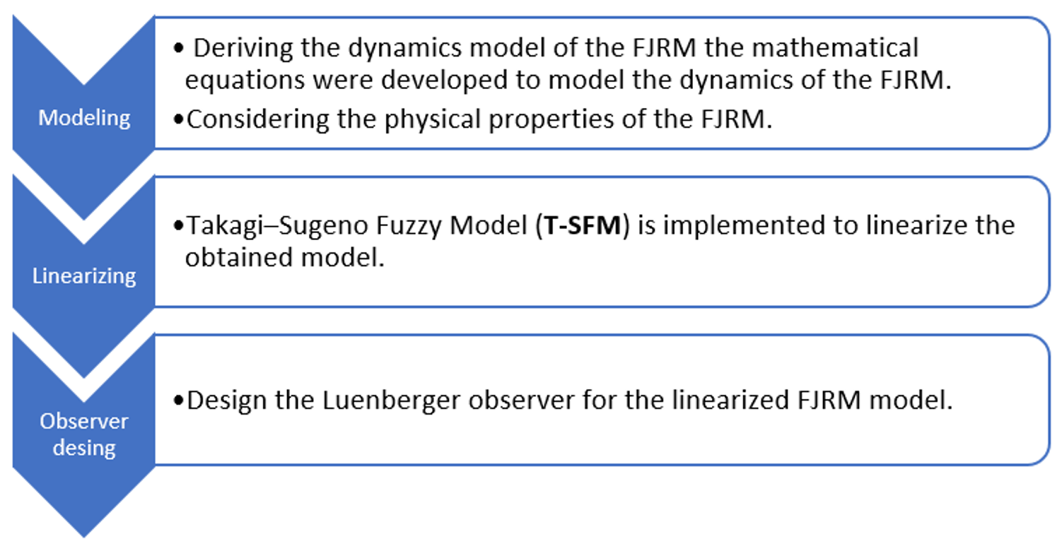
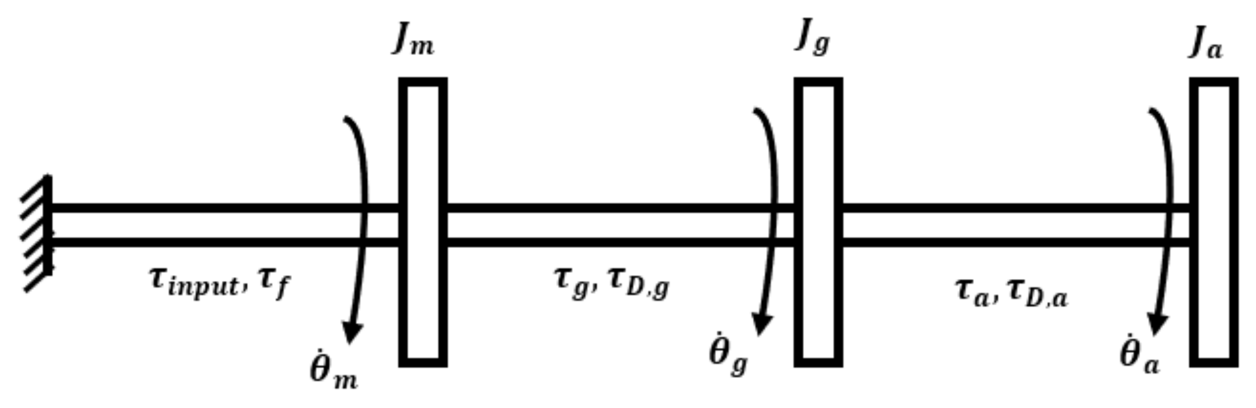
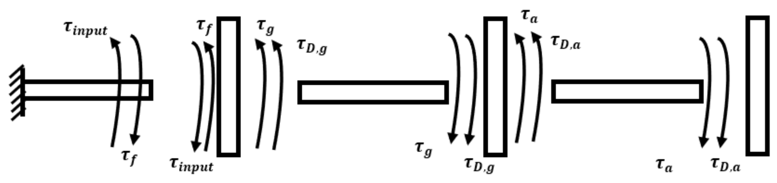
3. Mathematical Models

A nonlinear robotic arm (NRA) made of three non-rigid parts represents the FJRM considered in this study. The NRA, depicted in Figure 2, includes a motor for actuating the robot arm and driver gear for manipulating speed and changing rotation direction. The robotic arm has three rotational inertias, they are: motor of inertia $J_m$, driver gear of inertia $J_g$, and arm of inertial $J_a$. As shown in Figure 3, the dynamics model of the NRA includes three flexible parts. The first flexibility in Equation (1) is due to the effect of resisting the motion of the motor that is represented by the following static friction torque:

$${\tau }_f=F_v{\dot{\theta }}_m,$$

(1)

where $F_v$ denote the coefficient of viscosity of linear type. The second flexibility in Equation (2), located at the joint, is nonlinear due to the effect of driver gear of torsional torque value [25]:

$${\tau }_g=k_1\left({\theta }_m-{\theta }_g\right)+sign\left({\theta }_m-{\theta }_g\right)k_2{\left({\theta }_m-{\theta }_g\right)}^2+k_3{\left({\theta }_m-{\theta }_g\right)}^3,$$

(2)

the third flexibility in the arm structure in Equation (3) is considered linear in relation of torsional stiffness value:

$${\tau }_a=K_a\left({\theta }_g-{\theta }_a\right),$$

(3)

where $K_a$ is the linear stiffness of the arm. The damping coefficient is considered at the driver gear and arm of values $D_g$ and $D_a$. Hence, the torsional torque due to damping effect on the driver gear and arm are represented in Equations (4) and (5), respectively:

$${\tau }_{D,g}=D_g\left({\dot{\theta }}_m-{\dot{\theta }}_g\right),$$

(4)

$${\tau }_{D,a}=D_a\left({\dot{\theta }}_g-{\dot{\theta }}_a\right).$$

(5)

Figure 2. Nonlinear robotic arm drawing.

Figure 3. Nonlinear robotic arm dynamics model.

As it can be seen in Figure 4, the generalized coordinates of the NRA model are: rotation angle of the motor m, rotation angle of the gear $g$, and rotation angle of the arm. The free body diagram is depicted in Figure 4 to visualize all the torques that are exerted to the NRA body to determine reactions in dynamics analysis. Where input is the input torque of the motor that causes actuating the motion of the robot.

Figure 4. Nonlinear robotic arm free body diagram.

Consequently, assume Newton’s second law, the dynamics Equations (6)–(8) are derived as:

$$J_m{\ddot{\theta }}_m={\tau }_{input}-{\tau }_g-D_g\left({\dot{\theta }}_m-{\dot{\theta }}_g\right)-{\tau }_f,$$

(6)

$$J_g{\ddot{\theta }}_g={\tau }_g+D_g\left({\dot{\theta }}_m-{\dot{\theta }}_g\right)-D_a\left({\dot{\theta }}_g-{\dot{\theta }}_a\right)-K_a\left({\theta }_g-{\theta }_a\right),$$

(7)

$$J_a{\ddot{\theta }}_a=K_a\left({\theta }_g-{\theta }_a\right)+D_a\left({\dot{\theta }}_g-{\dot{\theta }}_a\right),$$

(8)

the next step is to derive the state space equations of the NRA model. Assuming the state variable vector $x=\left[\begin{array}{cccccc}{\theta }_m& {\theta }_g& {\theta }_a& {\dot{\theta }}_m& {\dot{\theta }}_g& {\dot{\theta }}_a\end{array}\right]$. Hence, considering the state vector and dynamics Equations (6) and (8), the state space Equations (9)–(14) are derived as:

$${\dot{x}}_1=x_4,$$

(9)

$${\dot{x}}_2=x_{5,}$$

(10)

$${\dot{x}}_3=x_{6,}$$

(11)

$${\dot{x}}_4=\frac{1}{J_m}\left[{\tau }_{input}-k_1\left(x_1-x_2\right)-sign\left(x_1-x_2\right)k_2{\left(x_1-x_2\right)}^2-k_3{\left(x_1-x_2\right)}^3-D_g\left(x_4-x_5\right)-F_v{x}_4\right],$$

(12)

$${\dot{x}}_5=\frac{1}{J_g}\left[k_1\left(x_1-x_2\right)+sign\left(x_1-x_2\right)k_2{\left(x_1-x_2\right)}^2+k_3{\left(x_1-x_2\right)}^3+D_g\left(x_4-x_5\right)-D_a\left(x_5-x_6\right)-K_a\left(x_2-x_3\right)\right],$$

(13)

$${\dot{x}}_6=\frac{1}{J_a}\left[K_a\left(x_2-x_3\right)+D_a\left(x_5-x_6\right)\right]$$

(14)

Assume the output of the NRA is the velocity of the arm, the output state Equation (15) can be written as:

$$y=x_4.$$

(15)

The derived state nonlinear equations will be used in the next section to linearize the nonlinear robotic arm using TS fuzzy models.

4. Dynamics Model Linearizing

Nonlinearity exists in the dynamics equations of various dynamics systems [26,27]. The linearization of the FJRM model is presented in this section. Nonlinear systems can be precisely linearized by applying T-SFM technique [28,29]. In this section, the T-SFM method of modeling will be applied to represent the high degree of nonlinear dynamics of the NRA in Equations (9)–(14) as a compact state space approach. The state space equation can be derived by rewriting the matrix form Equation (16) below:

$$\left[\begin{array}{c}{\dot{x}}_1\\ {\dot{x}}_2\\ {\dot{x}}_3\\ {\dot{x}}_4\\ {\dot{x}}_5\\ {\dot{x}}_6\end{array}\right]=\left[\begin{array}{cccccc}0& 0& 0& 1& 0& 0\\ 0& 0& 0& 0& 1& 0\\ 0& 0& 0& 0& 0& 1\\ a_{41}& a_{42}& 0& -\frac{1}{J_m}{D}_g-\frac{1}{J_m}{F}_v& \frac{1}{J_m}{D}_g& 0\\ a_{51}& a_{52}& K_a& \frac{1}{J_g}{D}_g+\frac{1}{J_g}{F}_v& -\frac{1}{J_g}{D}_g-\frac{1}{J_g}{D}_a& \frac{1}{J_g}{D}_a\\ 0& \frac{K_a}{J_a}& -\frac{K_a}{J_a}& 0& \frac{D_a}{J_a}& -\frac{D_a}{J_a}\end{array}\right]\left[\begin{array}{c}{x}_1\\ x_2\\ x_3\\ x_4\\ x_5\\ x_6\end{array}\right]+\left[\begin{array}{c}0\\ 0\\ 0\\ \frac{1}{J_m}\\ 0\\ 0\end{array}\right]{\tau }_{input},$$

(16)

where $a_{41}$, $a_{42}$, $a_{51}$, and $a_{52}$ represent the nonlinear components as bellow:

$$a_{41}=-\frac{1}{J_m}{k}_1-\frac{1}{J_m}sign\left(x_1-x_2\right)k_2{x}_1+2\frac{1}{J_m}sign\left(x_1-x_2\right)k_2{x}_2-\frac{1}{J_m}{k}_3 x^2{}_1+\frac{1}{J_m}{k}_3{x}^2{}_2,$$

$$a_{42}=\frac{1}{J_m}{k}_1-\frac{1}{J_m}sign\left(x_1-x_2\right)k_2{x}_2+3\frac{1}{J_m}{k}_3 x^2{}_1+\frac{1}{J_m}{k}_3{x}^2{}_2,$$

$$a_{51}=\frac{1}{J_g}{k}_1+\frac{1}{J_g}sign\left(x_1-x_2\right)k_2{x}_1-2\frac{1}{J_g}sign\left(x_1-x_2\right)k_2{x}_2+\frac{1}{J_g}{k}_3 x^2{}_1-\frac{1}{J_g}{k}_3{x}^2{}_2,$$

$$a_{52}=-\frac{1}{J_g}{k}_1+\frac{1}{J_g}sign\left(x_1-x_2\right)k_2{x}_2-3\frac{1}{J_g}{k}_3 x^2{}_1-\frac{1}{J_g}{k}_3{x}^2{}_2-\frac{1}{J_g}{K}_a.$$

Assume $Q_1=a_{41}$, $Q_2=a_{42}$, $Q_3=a_{51}$, $Q_4=a_{52}$. Then, the membership functions in Equations (17a)–(17d) are calculated as follows:

$$Q_1\left(t\right)=L_{1,Q_1}\mathrm{Max} \left[Q_1\right]+L_{2,Q_1}\mathrm{Min} \left[Q_1\right],$$

(17a)

$$Q_2\left(t\right)=L_{1,Q_2}\mathrm{Max} \left[Q_2\right]+L_{2,Q_2}\mathrm{Min} \left[Q_2\right],$$

(17b)

$$Q_3\left(t\right)=L_{1,Q_3}\mathrm{Max} \left[Q_3\right]+L_{2,Q_3}\mathrm{Min} \left[Q_3\right],$$

(17c)

$$Q_4\left(t\right)=L_{1,Q_4}\mathrm{Max} \left[Q_4\right]+L_{2,Q_4}\mathrm{Min} \left[Q_4\right],$$

(17d)

where:

$$L_{1,Q_1}+L_{2,Q_1}=1,$$

$$L_{1,Q_2}+L_{2,Q_2}=1,$$

$$L_{1,Q_3}+L_{2,Q_3}=1,$$

$$L_{1,Q_4}+L_{2,Q_4}=1$$

Hence, the membership functions are obtained as in Equations (18)–(25):

$$L_{1,Q_1}=\frac{Q_1\left(t\right)-\mathrm{Min} Q_1\left(t\right)}{\mathrm{Max} Q_1\left(t\right)-\mathrm{Min} Q_1\left(t\right)},$$

(18)

$$L_{2,Q_1}=\frac{-Q_1\left(t\right)+\mathrm{Max} Q_1\left(t\right)}{\mathrm{Max} Q_1\left(t\right)+\mathrm{Min} Q_1\left(t\right)},$$

(19)

$$L_{1,Q_2}=\frac{Q_2\left(t\right)-\mathrm{Min} Q_2\left(t\right)}{\mathrm{Max} Q_2\left(t\right)-\mathrm{Min} Q_2\left(t\right)},$$

(20)

$$L_{2,Q_2}=\frac{-Q_2\left(t\right)+\mathrm{Max} Q_2\left(t\right)}{\mathrm{Max} Q_2\left(t\right)+\mathrm{Min} Q_2\left(t\right)},$$

(21)

$$L_{1,Q_3}=\frac{Q_3\left(t\right)-\mathrm{Min} Q_3\left(t\right)}{\mathrm{Max} Q_3\left(t\right)-\mathrm{Min} Q_3\left(t\right)},$$

(22)

$$L_{2,Q_3}=\frac{-Q_3\left(t\right)+\mathrm{Max} Q_3\left(t\right)}{\mathrm{Max} Q_3\left(t\right)+\mathrm{Min} Q_3\left(t\right)},$$

(23)

$$L_{1,Q_4}=\frac{Q_4\left(t\right)-\mathrm{Min} Q_4\left(t\right)}{\mathrm{Max} Q_4\left(t\right)-\mathrm{Min} Q_4\left(t\right)},$$

(24)

$$L_{2,Q_4}=\frac{-Q_4\left(t\right)+\mathrm{Max} Q_4\left(t\right)}{\mathrm{Max} Q_4\left(t\right)+\mathrm{Min} Q_4\left(t\right)}$$

(25)

The membership functions $L_{1,Q_1}$, $L_{2,Q_1}$, $L_{1,Q_2}$, $L_{2,Q_2}$, $L_{1,Q_3}$, $L_{2,Q_3}$, $L_{1,Q_4}$, and $L_{2,Q_4}$ are named as ${“\mathrm{Q}}_1,\mathrm{Big}”$, ${“\mathrm{Q}}_1,\mathrm{small}”$, ${”\mathrm{Q}}_2,\mathrm{Big}”$, ${“\mathrm{Q}}_2,\mathrm{small}”$, ${“\mathrm{Q}}_3,\mathrm{Big}”$, ${“\mathrm{Q}}_3,\mathrm{small}”$, ${“\mathrm{Q}}_4,\mathrm{Big}”$, and ${“\mathrm{Q}}_4,\mathrm{small}”$, respectively.

In Table 2, all the rules are applied in terms of “IF and THEN” conditions. For instance, rule 4 is implemented as:

Table 2. Rules of the FJRM linearized model.

Module Rule Number	Linguistic Input				Linguistic Output
	${\mathit{Q}}_1\left(\mathit{t}\right)$	${\mathit{Q}}_2\left(\mathit{t}\right)$	${\mathit{Q}}_3\left(\mathit{t}\right)$	${\mathit{Q}}_4\left(\mathit{t}\right)$
1	${\mathrm{Q}}_1,\mathrm{Small}$	${\mathrm{Q}}_2,\mathrm{Small}$	${\mathrm{Q}}_3,\mathrm{Small}$	${\mathrm{Q}}_4,\mathrm{Small}$	$\dot{X}=A_{1}x\left(t\right)+B{\tau }_{input}$
2	${\mathrm{Q}}_1,\mathrm{Small}$	${\mathrm{Q}}_2,\mathrm{Small}$	${\mathrm{Q}}_3,\mathrm{Small}$	${\mathrm{Q}}_4,\mathrm{Big}$	$\dot{X}=A_{2}x\left(t\right)+B{\tau }_{input}$
3	${\mathrm{Q}}_1,\mathrm{Small}$	${\mathrm{Q}}_2,\mathrm{Small}$	${\mathrm{Q}}_3,\mathrm{Big}$	${\mathrm{Q}}_4,\mathrm{Small}$	$\dot{X}=A_{3}x\left(t\right)+B{\tau }_{input}$
4	${\mathrm{Q}}_1,\mathrm{Small}$	${\mathrm{Q}}_2,\mathrm{Small}$	${\mathrm{Q}}_3,\mathrm{Big}$	${\mathrm{Q}}_4,\mathrm{Big}$	$\dot{X}=A_{4}x\left(t\right)+B{\tau }_{input}$
5	${\mathrm{Q}}_1,\mathrm{Small}$	${\mathrm{Q}}_2,\mathrm{Big}$	${\mathrm{Q}}_3,\mathrm{Small}$	${\mathrm{Q}}_4,\mathrm{Small}$	$\dot{X}=A_{5}x\left(t\right)+B{\tau }_{input}$
6	${\mathrm{Q}}_1,\mathrm{Small}$	${\mathrm{Q}}_2,\mathrm{Big}$	${\mathrm{Q}}_3,\mathrm{Small}$	${\mathrm{Q}}_4,\mathrm{Big}$	$\dot{X}=A_{6}x\left(t\right)+B{\tau }_{input}$
7	${\mathrm{Q}}_1,\mathrm{Small}$	${\mathrm{Q}}_2,\mathrm{Big}$	${\mathrm{Q}}_3,\mathrm{Big}$	${\mathrm{Q}}_4,\mathrm{Small}$	$\dot{X}=A_{7}x\left(t\right)+B{\tau }_{input}$
8	${\mathrm{Q}}_1,\mathrm{Small}$	${\mathrm{Q}}_2,\mathrm{Big}$	${\mathrm{Q}}_3,\mathrm{Big}$	${\mathrm{Q}}_4,\mathrm{Big}$	$\dot{X}=A_{8}x\left(t\right)+B{\tau }_{input}$
9	${\mathrm{Q}}_1,\mathrm{Big}$	${\mathrm{Q}}_2,\mathrm{Small}$	${\mathrm{Q}}_3,\mathrm{Small}$	${\mathrm{Q}}_4,\mathrm{Small}$	$\dot{X}=A_{9}x\left(t\right)+B{\tau }_{input}$
10	${\mathrm{Q}}_1,\mathrm{Big}$	${\mathrm{Q}}_2,\mathrm{Small}$	${\mathrm{Q}}_3,\mathrm{Small}$	${\mathrm{Q}}_4,\mathrm{Big}$	$\dot{X}=A_{10}x\left(t\right)+B{\tau }_{input}$
11	${\mathrm{Q}}_1,\mathrm{Big}$	${\mathrm{Q}}_2,\mathrm{Small}$	${\mathrm{Q}}_3,\mathrm{Big}$	${\mathrm{Q}}_4,\mathrm{Small}$	$\dot{X}=A_{11}x\left(t\right)+B{\tau }_{input}$
12	${\mathrm{Q}}_1,\mathrm{Big}$	${\mathrm{Q}}_2,\mathrm{Small}$	${\mathrm{Q}}_3,\mathrm{Big}$	${\mathrm{Q}}_4,\mathrm{Big}$	$\dot{X}=A_{12}x\left(t\right)+B{\tau }_{input}$
13	${\mathrm{Q}}_1,\mathrm{Big}$	${\mathrm{Q}}_2,\mathrm{Big}$	${\mathrm{Q}}_3,\mathrm{Small}$	${\mathrm{Q}}_4,\mathrm{Small}$	$\dot{X}=A_{13}x\left(t\right)+B{\tau }_{input}$
14	${\mathrm{Q}}_1,\mathrm{Big}$	${\mathrm{Q}}_2,\mathrm{Big}$	${\mathrm{Q}}_3,\mathrm{Small}$	${\mathrm{Q}}_4,\mathrm{Big}$	$\dot{X}=A_{14}x\left(t\right)+B{\tau }_{input}$
15	${\mathrm{Q}}_1,\mathrm{Big}$	${\mathrm{Q}}_2,\mathrm{Big}$	${\mathrm{Q}}_3,\mathrm{Big}$	${\mathrm{Q}}_4,\mathrm{Small}$	$\dot{X}=A_{15}x\left(t\right)+B{\tau }_{input}$
16	${\mathrm{Q}}_1,\mathrm{Big}$	${\mathrm{Q}}_2,\mathrm{Big}$	${\mathrm{Q}}_3,\mathrm{Big}$	${\mathrm{Q}}_4,\mathrm{Big}$	$\dot{X}=A_{16}x\left(t\right)+B{\tau }_{input}$

IF ${\mathrm{Q}}_1,\mathrm{Small}$ and ${\mathrm{Q}}_2,\mathrm{Small}$ and ${\mathrm{Q}}_3,\mathrm{Big}$ and ${\mathrm{Q}}_4,\mathrm{Big}$ THEN $\dot{X}=A_{4}x\left(t\right)+B{\tau }_{input}$.

All the other rules are applied in the same way. The outcome of the fuzzy inference is then defuzzied to provide the final result of exactly representing the FJRM in Equations (26) and (27) and as:

$$\dot{X}={\displaystyle \sum }_{i=1}^{16}{h}_{i,NRA}\left(Q\right)\left(A_{i}x\left(t\right)+B_i{\tau }_{input}\right),$$

(26)

$$y={\displaystyle \sum }_{i=1}^{16}{h}_{i,NRA}\left(Q\right)C_{i}x\left(t\right).$$

(27)

where $h_{i,NRA}$ is calculated again from Table 1. For example, $h_{13,NRA}={\mathrm{Q}}_1,\mathrm{Big}\times {\mathrm{Q}}_2,\mathrm{Big}\times {\mathrm{Q}}_3,\mathrm{Small}\times {\mathrm{Q}}_4,\mathrm{Small}$. The obtained linearized model of the FJRM will be used in the next section to design the observer.

5. Observer Design

Observers are implemented to reduce the number of sensors in the target device [30,31]. The transmission model of the dynamics system of the FJRM includes the states function $f_{\mathrm{FJRM}}$ and the measurement function $h_{\mathrm{FJRM}}$. They can be represented by the following general dynamics expressions in Equations (28) and (29) and:

$$\dot{x}\left(t\right)=f_{\mathrm{FJRM}}\left(x\left(t\right),{\tau }_{input}\right),$$

(28)

$$y\left(t\right)=h_{\mathrm{FJRM}}\left(x\left(t\right),{\tau }_{input}\right)$$

(29)

An observer is essential to be considered when the output of the FJRM system $y\left(t\right)$ is not identical to the value of the state variable $x\left(t\right)$. In fact, it is not possible to observe the states of nonlinear systems directly. In turn, the nonlinear FJRM dynamics model in Equation (16) is linearized using T-SFM model technique as explained in Section 4 that is represented by the final formula in Equations (26) and (27). In this section, the observer design is presented and the analysis of stability is applied. As a first step, it is assumed the estimated vector of state, measured variable, and scheduling are $\widehat{x}$, $\widehat{y}$, and $\widehat{Q}$, respectively. On the other hand, the gain of the observer is considered as $G_{i,NRA}\left(y-\widehat{y}\right)$. The objective of the observer is to asymptotically reduce the estimation error, $E_{NRA}=x\left(t\right)-\widehat{x}$, to zero as the time go to infinity. Refereeing to the linearized model in Equations (26) and (27), the general form of the applied observer [32] in Equation (30) is:

$$\dot{\widehat{X}}={\displaystyle \sum }_{i=1}^n{h}_{i,NRA}\left(\widehat{Q}\right)\left(A_i\widehat{x}\left(t\right)+B_i{\tau }_{input}+G_{i,NRA}\left(y-\widehat{y}\right)\right),$$

(30)

$$\widehat{y}=C\widehat{x}\left(t\right),$$

(31)

and the dynamics of error is

$${\dot{E}}_{NRA}=\dot{x}\left(t\right)-\widehat{\dot{x}},$$

(32)

$${\dot{E}}_{NRA}={\displaystyle \sum }_{i=1}^n{h}_{i,NRA}\left(\widehat{Q}\right)\left(A_i-G_{i,NRA}C\right)E_{NRA}+{\displaystyle \sum }_{i=1}^n\left(h_{i,NRA}\left(Q\right)-h_{i,NRA}\left(\widehat{Q}\right)\right)\left(A_{i}x\left(t\right)+B_i{\tau }_{input}\right),$$

(33)

where $n$ is the number of rules of modules which equals 16 (n = 16) as shown in Table 1. This observer is formulated in a way that all the rules explained in Table 1 are locally used. Hence, it is essential to ensure that the local models are observed, i.e., $A_i$ and $C_i$, instead of the original nonlinear dynamics model of the FJRM. The scheduling vector that includes ${\mathrm{Q}}_{\mathrm{i}}$ where $i=1,\dots ,4$, according to the system of the FJRM in Equations (26) and (27), depends on the states that are unmeasured. Consequently, the estimated values ${\widehat{\mathrm{Q}}}_1$, ${\widehat{\mathrm{Q}}}_2$, ${\widehat{\mathrm{Q}}}_3$, and ${\widehat{\mathrm{Q}}}_4$ are implemented rather than the true ones while the only one measurement matrix $C$ is applied. However, the error of the FJRM system of Equation (33) is exponentially stable when the inequity in Equation (34) is achieved:

$$\Vert \left(h_{i,NRA}\left(Q\right)-h_{i,NRA}\left(\widehat{Q}\right)\right)\left(A_{i}x\left(t\right)+B_i{\tau }_{input}\right)\Vert \le \beta \Vert E_{NRA}\Vert ,$$

(34)

where $\beta$ is a positive constant number that can be determined by applying the following optimization formula [33] in Equation (35):

$$\beta =\Vert \frac{\partial \left(h_{i,NRA}\left(Q\right)-h_{i,NRA}\left(\widehat{Q}\right)\right)\left(A_{i}x\left(t\right)+B_i{\tau }_{input}\right)}{\partial E_{NRA}}\Vert .$$

(35)

The structure of the observer has been established in this section. By comparing Equations (26) and (30), the observer can be designed within the presented methods of this study taking in consideration the dynamics error in Equation (33).

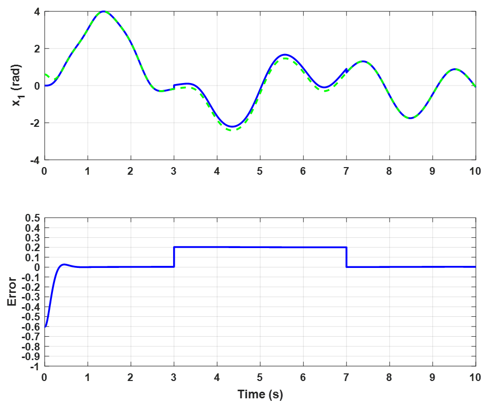
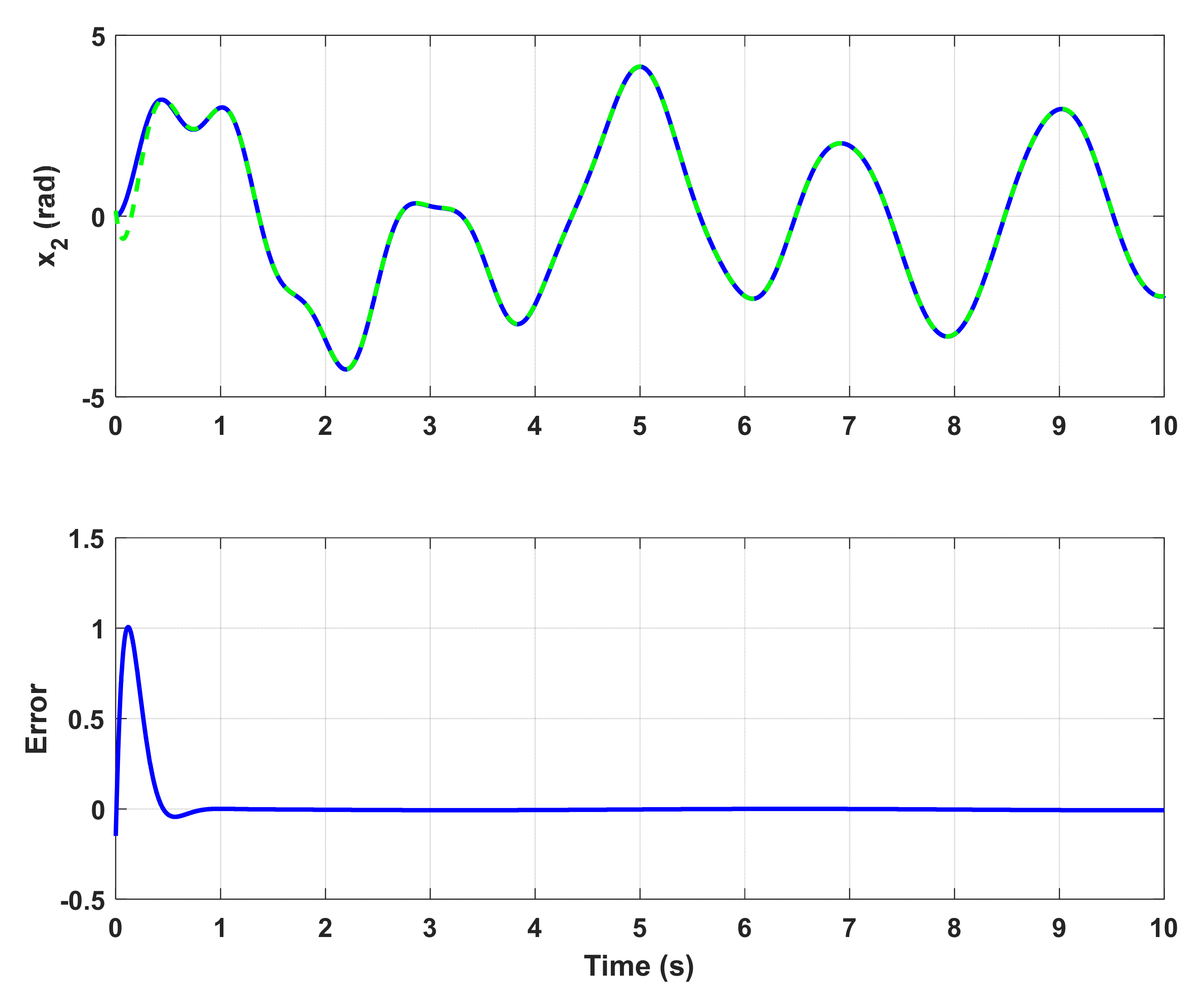
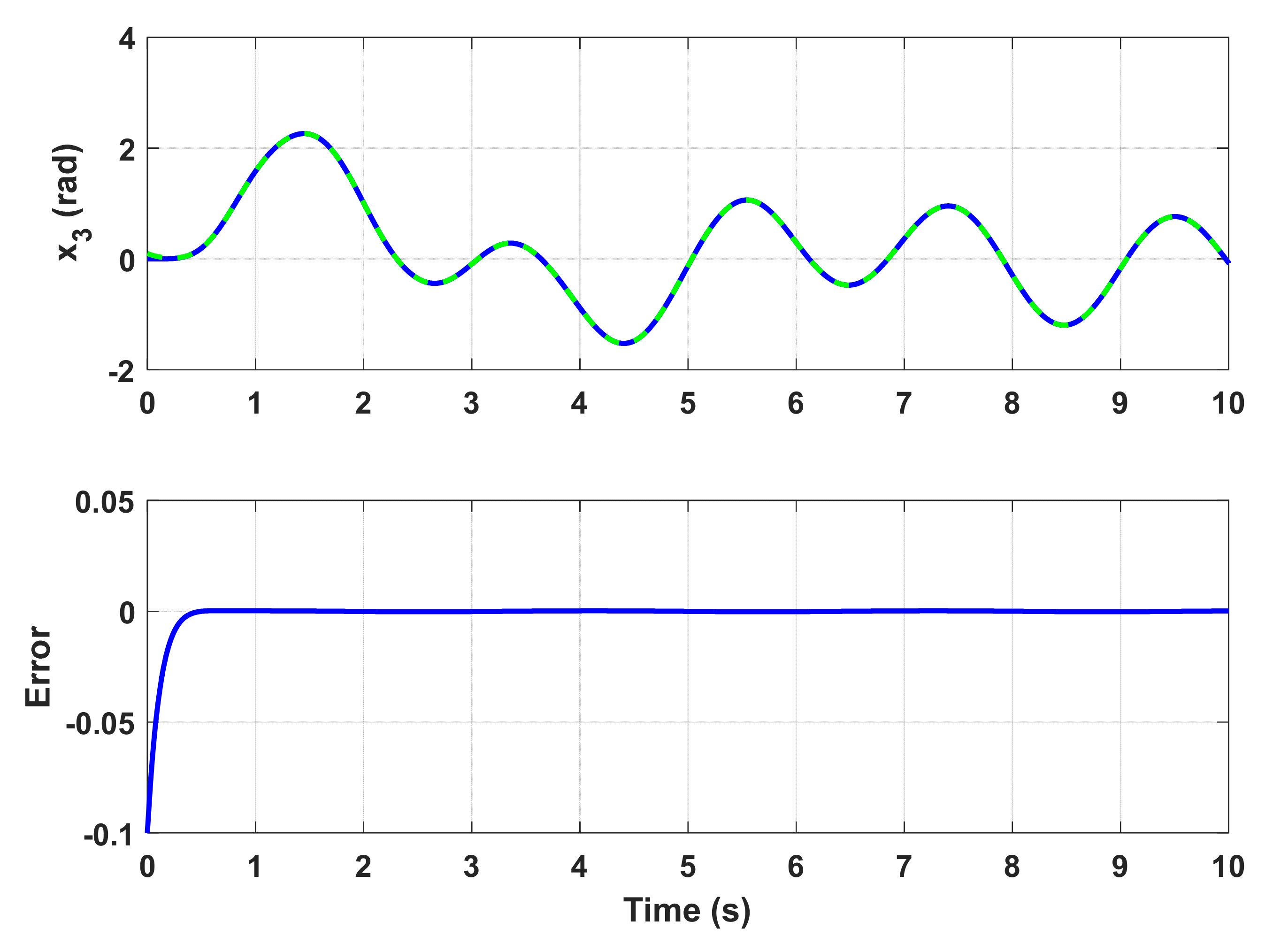
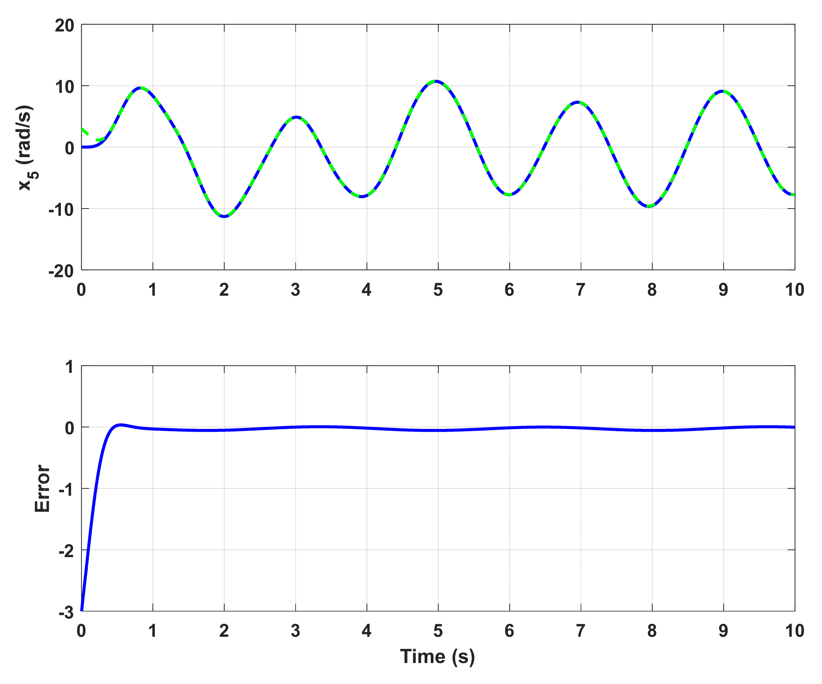
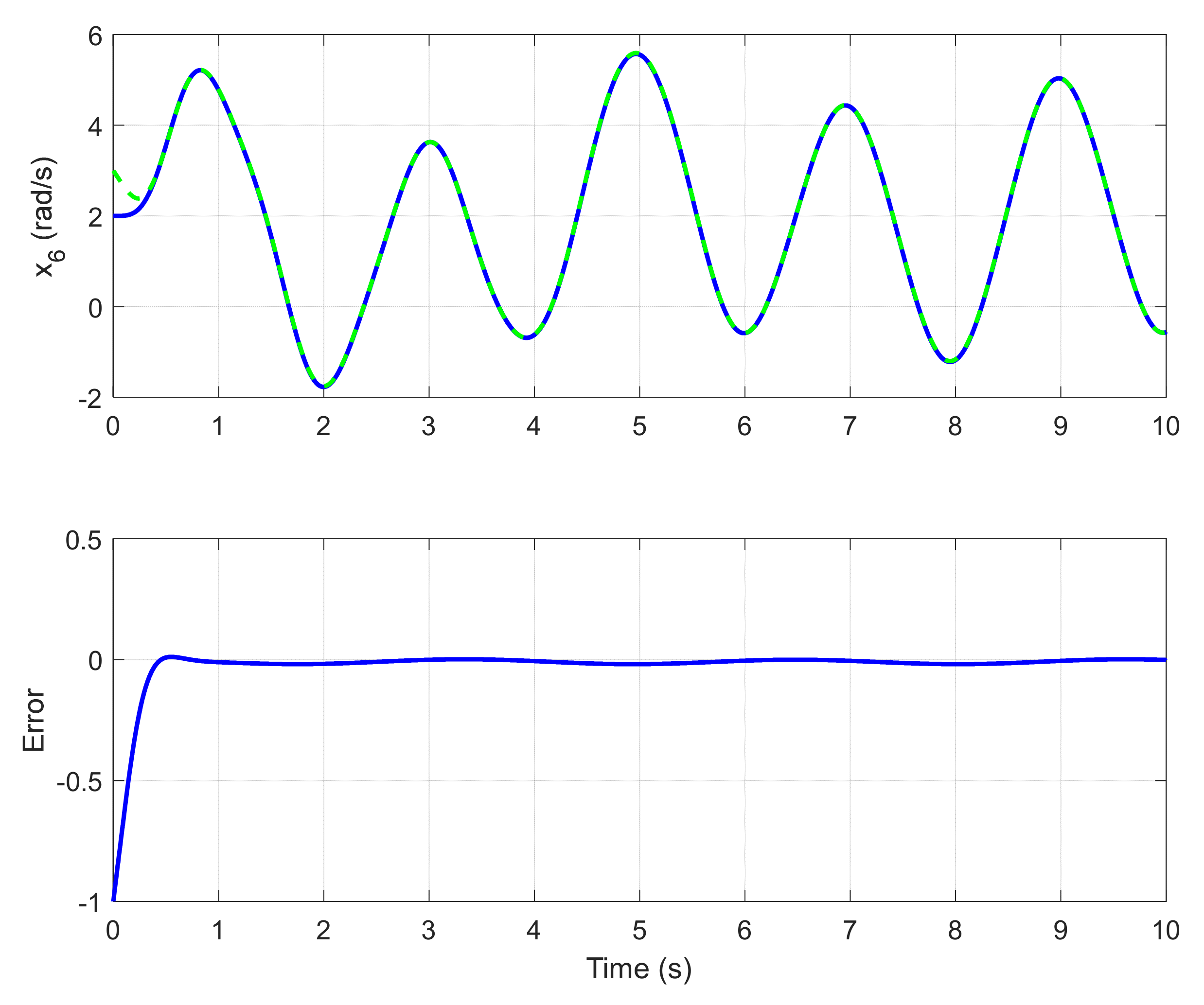
6. Simulation Results

The following case study is considered in order to evaluate the suggested Luenberger observer. Assuming the physical FJRM parameters of Table 3, then, Equation (16) will become as in the following Equation (36):

$$\left[\begin{array}{c}{\dot{x}}_1\\ {\dot{x}}_2\\ {\dot{x}}_3\\ {\dot{x}}_4\\ {\dot{x}}_5\\ {\dot{x}}_6\end{array}\right]=\left[\begin{array}{cccccc}0& 0& 0& 1& 0& 0\\ 0& 0& 0& 0& 1& 0\\ 0& 0& 0& 0& 0& 1\\ a_{41}& a_{42}& 0& -5.47& 5.45& 0\\ a_{51}& a_{52}& 5.3& 0.82& 3.1& 2.27\\ 0& 497.7& -407.7& 0& 7.7& -7.7\end{array}\right]\left[\begin{array}{c}{x}_1\\ x_2\\ x_3\\ x_4\\ x_5\\ x_6\end{array}\right]+\left[\begin{array}{c}0\\ 0\\ 0\\ 151.5\\ 0\\ 0\end{array}\right]{\tau }_{input},$$

(36)

where:

$$a_{41}=-25.75-30.3sign\left(x_1-x_2\right)x_1+60.6sign\left(x_1-x_2\right)x_2-31.8 x^2{}_1+31.8x^2{}_2,$$

$$a_{42}=25.75-30.3sign\left(x_1-x_2\right)x_2+95.45 x^2{}_1+31.8x^2{}_2,$$

$$a_{51}=3.8+4.5sign\left(x_1-x_2\right)x_1-66.6sign\left(x_1-x_2\right)x_2+4.77 x^2{}_1-4.77x^2{}_2,$$

$$a_{52}=-3.8+4.54sign\left(x_1-x_2\right)x_2-14.3 x^2{}_1-4.7x^2{}_2-120.4.$$

Table 3. Suggested NRA parameters [34].

NRA Physical Parameter	Value	Unit
$J_m$	0.0059	$\mathrm{kg}\times {\mathrm{m}}^2$
$J_g$	0.0201	$\mathrm{kg}\times {\mathrm{m}}^2$
$J_a$	0.00687	$\mathrm{kg}\times {\mathrm{m}}^2$
$k_1$	0.0206	$\mathrm{N}/\mathrm{m}$
$k_2$	0.02	$\mathrm{N}/\mathrm{m}$
$k_3$	0.021	$\mathrm{N}/\mathrm{m}$
$K_a$	0.0202	$\mathrm{N}/\mathrm{m}$
$D_g$	0.0624	$\mathrm{N}\times \mathrm{s}/\mathrm{m}$
$D_a$	0.00988	$\mathrm{N}\times \mathrm{s}/\mathrm{m}$
$F_v$	0.000986	Unitless

The membership functions are determined according to Equations (18)–(25) and the minimum and maximum values of Qi of Table 4, where I = 1, …, 4.

Table 4. Proposed range values of state variables.

State Parameter	Description (Unit)	Minimum Range	Maximum Range
$x_1$	Motor angle (rad)	0	$2\pi$
$x_2$	Driver gear angle (rad)	0	$2\pi$
$x_3$	Arm angle (rad)	0	$\pi /2$
$x_4$	Motor rate (rad/s)	0	60
$x_5$	Driver gear rate (rad/s)	0	60
$x_6$	Arm rate (rad/s)	0	60

The stable Luenberger observer with the optimization formula of Equation (35) is designed based on Equation (30) where the rate of error of Equation (33) is minimized to zero. For input torque ${\tau }_{input}=\sin \pi t$, the simulation results are presented in Figure 5, Figure 6, Figure 7, Figure 8 and Figure 9. In these Figures, the solid blue line represents the real value of the state while the dashed green line represents the estimated value of the observer. In each figure, the error is calculated as the difference between the real and estimated values of the state. Assuming ${\widehat{x}}_i$ is the estimated of the corresponding state $x_i$. Then, in Equation (37), the percentage of the relative error is defined as:

$$\% error\_x_i=\frac{x_i-{\widehat{x}}_i}{x_i}$$

(37)

Figure 5. Estimation and error of motor angle.

Figure 6. Estimation and error of driver gear angle.

Figure 7. Estimation and error of arm angle.

Figure 8. Estimation and error of driver gear rate.

Figure 9. Estimation and error of arm rate.

Applying Equation (37) to the results of Figure 5, Figure 6, Figure 7, Figure 8 and Figure 9, the percentage of the relative error of each estimated signal are calculated as:

$$\%erro{r}_{x_1}=5\%$$

$$\%erro{r}_{x_2}=2\%$$

$$\% erro{r}_{x_3}=2.5\%$$

$$\% erro{r}_{x_4}=3\%$$

$$\% erro{r}_{x_6}=2\%$$

The results show the ability of the proposed observer to estimate the state variables of the FJRM system with zero errors. The dynamics of the observer are quite satisfactory, no overshooting with accurate tracking which demonstrate the efficiency of the designed observer. Since the designed observer used the linearized FJRM model without any errors we can derive that T-SFM technique is suitable for this type of problems.

7. Conclusions

In this study, a fuzzy Luenberger observer based on the T-SFM approach for FJRM has been introduced. The nonlinear model of the FJRM was derived in the form of a state space model, in which the nonlinearity was assumed to be of 3rd order in the joint of the robot. The nonlinear model was linearized using the T-SFM approach to precisely represent the FJRM system in terms of linear state model. The unmeasured states were estimated by the designed Leunberger observer. The developed observer showed its ability to control the FJRM by utilizing only one measured signal which was the velocity of the motor. Stability analysis was implemented to ensure the ability of the designed observer to stabilize the FJRM system. Simulation results verify the effectiveness of the presented observer to estimate the states of the FJRM with zero steady errors. The dynamics of the observer are quite satisfactory, no overshooting with accurate tracking which demonstrate the efficiency of the designed observer The main limitation of this work is that only the T-SFM technique was used, however, it was proven to be suitable as it produced zero errors. As a future work, it is recommended to apply the developed observer of this study to a practical FJRM system.

References

1. García, P.L.; Crispel, S.; Saerens, E.; Verstraten, T.; Lefeber, D. Compact Gearboxes for Modern Robotics: A Review. Front. Robot. AI 2020, 7, 1–20. [Google Scholar] [CrossRef] [PubMed]
2. Sinitcyna, Y.V.; Ermolaev, M.M. Influence of Bearing’s Flexibility on the Working of Cycloid Drive. IOP Conf. Ser. Mater. Sci. Eng. 2020, 842, 012021. [Google Scholar] [CrossRef]
3. Gaiser, I.; Wiegand, R.; Ivlev, O.; Andres, A.; Breitwieser, H.; Schulz, S.; Bretthauer, G. Compliant Robotics and Automation with Flexible Fluidic Actuators and Inflatable Structures. 2012. Available online: https://www.intechopen.com/chapters/40057 (accessed on 15 March 2022).
4. Reutov, A. Modeling of the flexible belt motion on the drive pulley of woodworking equipment. IOP Conf. Ser. Earth Environ. Sci. 2019, 392, 012056. [Google Scholar] [CrossRef]
5. Yang, W.; Yuan, H.; Li, H.; Zhang, K. Dynamic Analysis of Flexible Shaft and Elastic Disk Rotor System Based on the Effect of Alford Force. Shock Vib. 2019, 2019, 3545939. [Google Scholar] [CrossRef]
6. Al-Darraji, I.; Kılıç, A.; Kapucu, S. Optimal control of compliant planar robot for safe impact using steepest descent technique. In Proceedings of the International Conference on Information and Communication Technology (ICICT ’19), Baghdad, Iraq, 15–16 April 2019; Association for Computing Machinery: New York, NY, USA, 2019; pp. 233–238. [Google Scholar] [CrossRef]
7. Korayem, M.H.; Heidari, H.R. Modeling and testing of moving base manipulators with elastic joints. Latin Am. Appl. Res. 2011, 41, 157–163. [Google Scholar]
8. Gao, M.; Wang, Z.; Pang, Z.; Sun, J.; Li, J.; Li, S.; Zhang, H. Electrically Driven Lower Limb Exoskeleton Rehabilitation Robot Based on Anthropomorphic Design. Machines 2022, 10, 266. [Google Scholar] [CrossRef]
9. Righettini, P.; Strada, R.; Cortinovis, F. Modal Kinematic Analysis of a Parallel Kinematic Robot with Low-Stiffness Transmissions. Robotics 2021, 10, 132. [Google Scholar] [CrossRef]
10. Fu, X.; Ai, H.; Chen, L. Repetitive Learning Sliding Mode Stabilization Control for a Flexible-Base, Flexible-Link and Flexible-Joint Space Robot Capturing a Satellite. Appl. Sci. 2021, 11, 8077. [Google Scholar] [CrossRef]
11. Shao, M.; Huang, Y.; Vadim, V. Silberschmidt, Intelligent Manipulator with Flexible Link and Joint: Modeling and Vibration Control. Shock Vib. 2020, 2020, 4671358. [Google Scholar] [CrossRef] [Green Version]
12. Ott, C. Modeling of Flexible Joint Robots. In Cartesian Impedance Control of Redundant and Flexible-Joint Robots; Springer Tracts in Advanced Robotics; Springer: Berlin/Heidelberg, Germany, 2008; Volume 49. [Google Scholar] [CrossRef]
13. Wang, H.; Xiao, P. Simulation of Manipulator with Flexible Joint. In Applied Mechanics and Materials; Trans Tech Publications, Ltd.: Freinbach, Switzerland, 2013; pp. 999–1003. [Google Scholar]
14. Ghorbel, F.; Hung, J.Y.; Spong, M.W. Adaptive control of flexible-joint manipulators. IEEE Control Syst. Mag. 1989, 9, 9–13. [Google Scholar] [CrossRef]
15. Aziz, H.; Iqbal, J. Flexible Joint Robotic Manipulator: Modeling and Design of Robust Control Law (Best Paper Award). 2016. Available online: https://ieeexplore.ieee.org/document/7791230 (accessed on 22 December 2016).
16. Pavlichenko, D.; Behnke, S. Flexible-Joint Manipulator Trajectory Tracking with Learned Two-Stage Model employing One-Step Future Prediction. In Proceedings of the Fifth IEEE International Conference on Robotic Computing (IRC), Taichung, Taiwan, 15–17 November 2021. [Google Scholar]
17. Ahmadi, S.; Fateh, M. Control of flexible joint robot manipulators by compensating flexibility. Iran. J. Fuzzy Syst. 2018, 15, 57–71. [Google Scholar] [CrossRef]
18. Zhang, A.; Lin, Z.; Wang, B.; Han, Z. Nonlinear Model Predictive Control of Single-Link Flexible-Joint Robot Using Recurrent Neural Network and Differential Evolution Optimization. Electronics 2021, 10, 2426. [Google Scholar] [CrossRef]
19. Abdollahi, F.; Talebi, H.A.; Patel, R.V. A stable neural network-based observer with application to flexible-joint manipulators. IEEE Trans. Neural Netw. 2006, 17, 118–129. [Google Scholar] [CrossRef] [PubMed]
20. Nicosia, S.; Tomei, P.; Tornambe, A. A nonlinear observer for elastic robots. IEEE J. Robot. Auto 1988, 4, 45–52. [Google Scholar] [CrossRef]
21. De Luca, A.; Schroder, D.; Thummel, M. An Acceleration-based State Observer for Robot Manipulators with Elastic Joints. In Proceedings of the 2007 IEEE International Conference on Robotics and Automation, Rome, Italy, 10–14 April 2007; pp. 3817–3823. [Google Scholar] [CrossRef]
22. Filipescu, A.; Dugard, L.; Dion, J. Flexible Joints Robotic Manipulator Control by Adaptive Gain Smooth Sliding Observer-Controller. Fascicle III, Electrotechnics, Electronics, Automatic Control, Informatics. In The Annals of “Dunarea de Jos” University of Galati; Galati University Press: Galati, Romania, 2003; Volume 26, pp. 5–13. [Google Scholar]
23. Bona, B.; Indri, M. Analysis and implementation of observers for robotic manipulators. In Proceedings of the 1998 IEEE International Conference on Robotics and Automation (Cat. No.98CH36146), Leuven, Belgium, 20–20 May 1998; Volume 4, pp. 3006–3011. [Google Scholar] [CrossRef]
24. Ullah, H.; Malik, F.M.; Raza, A.; Mazhar, N.; Khan, R.; Saeed, A.; Ahmad, I. Robust Output Feedback Control of Single-Link Flexible-Joint Robot Manipulator with Matched Disturbances Using High Gain Observer. Sensors 2021, 21, 3252. [Google Scholar] [CrossRef] [PubMed]
25. Seyfferth, W.; Maghzal, A.J.; Angeles, J. Nonlinear modeling and parameter identification of harmonic drive robotic transmissions. In Proceedings of the 1995 IEEE International Conference on Robotics and Automation, Nagoya, Japan, 21–27 May 1995; Volume 3, pp. 3027–3032. [Google Scholar] [CrossRef]
26. Al-Darraji, I.; Piromalis, D.; Kakei, A.A.; Khan, F.Q.; Stojmenovic, M.; Tsaramirsis, G.; Papageorgas, P.G. Adaptive Robust Controller Design-Based RBF Neural Network for Aerial Robot Arm Model. Electronics 2021, 10, 831. [Google Scholar] [CrossRef]
27. Al-Darraji, I.; Derbali, M.; Tsaramirsis, G. Tilting-rotors Quadcopters: A New Dynamics Modelling and Simulation based on the Newton-Euler Method with Lead Compensator Control. In Proceedings of the 2021 8th International Conference on Computing for Sustainable Global Development (INDIACom), New Delhi, India, 17–19 March 2021; pp. 363–369. [Google Scholar] [CrossRef]
28. Al-Darraji, I.; Kakei, A.A.; Ismaeel, A.G.; Tsaramirsis, G.; Khan, F.Q.; Randhawa, P.; Alrammal, M.; Jan, S. Takagi–sugeno fuzzy modeling and control for effective robotic manipulator motion. Comput. Mater. Contin. 2022, 71, 1011–1024. [Google Scholar]
29. Jerbi, H.; Kchaou, M.; Boudjemline, A.; Regaieg, M.A.; Ben Aoun, S.; Kouzou, A.L. H∞ and Passive Fuzzy Control for Non-Linear Descriptor Systems with Time-Varying Delay and Sensor Faults. Mathematics 2021, 9, 2203. [Google Scholar] [CrossRef]
30. Kchaou, M.; Jerbi, H.; Ali, N.B.; Alsaif, H. H∞ Reliable Dynamic Output-Feedback Controller Design for Discrete-Time Singular Systems with Sensor Saturation. Actuators 2021, 10, 196. [Google Scholar] [CrossRef]
31. Regaieg, M.A.; Kchaou, M.; Jerbi, H.; Boudjemline, A.; Hafaifa, A. Robust Asynchronous H∞ Observer-Based Control Design for Discrete-Time Switched Singular Systems with Time-Varying Delay and Sensor Saturation: An Average Dwell Time Approach. Electronics 2021, 10, 2334. [Google Scholar] [CrossRef]
32. Nandam, P.K.; Sen, P.C. A comparative study of a Luenberger observer and adaptive observer-based variable structure speed control system using a self-controlled synchronous motor. IEEE Trans. Indust. Electron. 1990, 37, 127–132. [Google Scholar] [CrossRef]
33. Mohan, S.; Liu, J.; Vasudevan, R. Synthesizing the optimal luenberger-type observer for nonlinear systems. In Proceedings of the 2017 IEEE 56th Annual Conference on Decision and Control (CDC), Melbourne, VIC, Australia, 12–15 December 2017; pp. 3658–3663. [Google Scholar] [CrossRef] [Green Version]
34. Wernholt, E.; Gunnarsson, S. Nonlinear Identification of a Physically Parameterized Robot Model 1; IFAC Proceedings Volumes; Linköpings Universitet: Linköping, Sweden, 2006; Volume 39, pp. 143–148. ISBN 9783902661029. [Google Scholar]
Publisher’s Note: MDPI stays neutral with regard to jurisdictional claims in published maps and institutional affiliations.
Article Metrics
Citations
Article Access Statistics
Multiple requests from the same IP address are counted as one view.