Cinematographic Shot Classification with Deep Ensemble Learning

Abstract

Cinematographic shot classification assigns a category to each shot either on the basis of the field size or on the movement performed by the camera. In this work, we focus on the camera field of view, which is determined by the portion of the subject and of the environment shown in the field of view of the camera. The automation of this task can help freelancers and studios belonging to the visual creative field in their daily activities. In our study, we took into account eight classes of film shots: long shot, medium shot, full figure, american shot, half figure, half torso, close up and extreme close up. The cinematographic shot classification is a complex task, so we combined state-of-the-art techniques to deal with it. Specifically, we finetuned three separated VGG-16 models and combined their predictions in order to obtain better performances by exploiting the stacking learning technique. Experimental results demonstrate the effectiveness of the proposed approach in performing the classification task with good accuracy. Our method was able to achieve 77% accuracy without relying on data augmentation techniques. We also evaluated our approach in terms of f1 score, precision, and recall and we showed confusion matrices to show that most of our misclassified samples belonged to a neighboring class.

1. Introduction

Images and videos belong to different cinematographic shots according to what is shown in the field size of the camera. This type of classification is the main typology used in the creative field to classify images or videos. The benefits of automating such a task are many and cover many sub-areas of the creative world. Information concerning the types of shot used can offer insight on different aspects for movie analysis [1], from stylistic aspects to narrative ones [2]. In ref. [3], for example, the authors perform an automatic attribution of authorship of films by analyzing two features: the recording time and the cinematographic shot class. In this way, they can gain interesting insights into the differences between the editing styles of different directors. The cinematographic shot classification can also be used in practical applications. For example, it can be used to reduce the time needed to edit a video or to automatically organize large image archives. Usually, in the creative field, especially for large projects, you have to work with a huge amount of unorganized data. If the data are organized, it means that someone has organized it manually, which is a tedious and time-consuming task. Automated methods should be developed to help freelancers and experts in the creative field to classify their image archives easily and quickly.

Here, we present an innovative deep learning approach for effective classification of cinematographic shots. This task is complex due to several similar aspects between some classes. Compared to other image classification tasks the cinematographic shot classification presents a couple of peculiarities. While some of the cinematographic shot classes have a lot of identifying patterns in common, some other classes have a lot of totally different identifying patterns.

For instance, a long shot is a long shot if it does not contain humans but it is the same if what is shown is a desert, the ocean or a forest. On the other hand there are some elements that can appear in different types of shot. For instance a tree in the background can appear in a long shot and also in a full figure. The different types of shot considered for this study are shown in Figure 1. Here is a brief description of the shots considered:

Figure 1. The eight types of shots considered.

• Long Shot (LS): a shot in which the human figure can be absent or occupy less than a third of the screen height
• Medium Shot (MS): a shot in which the human figure occupies from a third to two thirds of the screen height
• Full Figure (FF): a shot in which the human figure occupies from two thirds to the totality of the screen height
• American Shot (AS): a shot in which the human figure is cut around the knee
• Half Figure (HF): a shot in which the only the upper half of the human figure is shown
• Half Torso (HT): a shot in which the human figure is shown from the upper chest to the head
• Close Up (CU): a shot in which the subject is shown from the shoulders to the head
• Extreme Close Up (ECU): a shot in which the face of the subject occupies most of the image

Due to the complexity of the problem innovative approaches are required. Instead of adopting regular data augmentation techniques we augmented the data by exploiting other neural networks. By doing so, we were able to create two alterations of the original dataset. At this point, we finetuned three different pre-trained VGG-16 models, each one with a different dataset. After tuning the networks, we combined their predictions using the stacking learning technique, an ensemble learning technique [4]. Stacking learning refers to a specific type of ensemble learning. Ensemble Learning combines predictions from different models. When the predictions are combined using another classifier instead of majority voting or average voting, we used stacking learning.

The main contribution of this research are the following:

• a two-stage classification task based on three parallel CNN models using three different representations of the dataset (original, stylized and hypercolumns) and a stacking learning strategy to correctly classify different classes of movie shots.
• an intensive experimental test with a large amount of real movie footage belonging to 8 classes to show the effectiveness of the proposed approach in correctly classifying cinematographic shots.
• the creation of a new large dataset of 10,545 images divided into eight classes of interest.
• an adaptation of the proposed approach on a different classification task.

This paper is organized as follows. In Section 2, we discuss the literature review. Section 3 analyzes the different datasets used in this study, while Section 4 presents the proposed methodology. Section 5 presents the results obtained and some comparisons with state-of-the-art techniques. Finally, Section 6 presents the conclusions.

2. Related Works

During the past few years, the attention paid to cinematographic shot classification has grown. Some studies [1,5,6,7] focus directly on possible interactions between the shot classification and machine learning techniques, while others [8,9,10] implement different strategies.

The authors in [5] addressed this task focusing on macro groups of shots, i.e., long shots, medium shots and close ups. In this study, the authors extract specific features and then feed them to classification models. The authors reached an accuracy of 84% using as classifier a Support Vector Machine (SVM). Also the authors in [2] classify the shots into long shots, medium shots and close ups, but they use a convolutional neural network as classifier, reaching an accuracy of 94%.

In ref. [7], the authors manage to classify images into the following seven types of shots: extreme long shot, long shot, medium long shot, medium shot, medium close up, close up and extreme close up. In this work the the authors used the head size and its position to perform the classification. They used a semi-automatic face tracker to estimate the size and the position of a head inside the frame. After assessing these two features the shots are classified by an SVM. In ref. [11] a VGG-16 has been used to classify images into cinematographic shots; however, the classes considered were only four. In ref. [1], the authors use semantic segmentation on images and then feed them to a ResNet-50. The classes considered in this study are only three, i.e., close up, medium shot and long shot. Using a ResNet-50 as classifier the authors reached an accuracy of 96%.

In ref. [8], the authors focus on the camera movement and classify the shots accordingly. So, instead of labeling the shots as long shot, medium shot and so on, they classify them as static, tilt, pan and zoom. They perform such operation thanks to a motion vector field. Other studies that focus on the motion semantics rather than the field of view of the camera are [9,10]. A recent interesting study [12] classifies camera movements and a small amount of shots, i.e., long shot, full shot, medium shot, close-up and extreme close-up. They used a huge dataset containing over 46,000 images. In order to perform the classification they proposed a learning framework called Subject Guidance Network (SGNet). It splits the subject and the background of a shot into two streams, serving as separate guidance maps for scale and movement type classification, respectively. In [13], ensemble learning was used with convolutional neural networks to classify images; however, it was for a different image classification task. Moreover, there was no alteration in the different datasets used. In ref. [14], they have used different alterations of the images using the style transfer technique. They proved the before mentioned higher sensibility of CNNs to texture patterns. In ref. [15], the authors present MovieNet, a dataset intended to address movie understanding. The dataset can be used to address different tasks, among which there is the cinematographic shot classification. The classes considered in this paper are the long shot, full shot, medium shot, close up and extreme close up. The classification accuracy reached is 87.5%.

Indeed, there are two main approaches to the cinematographic shot classification, one based on the field of view of the camera while the other one focuses on the camera movement. The work proposed in this paper differs from those works that focus on the camera field of view for the methodology used and the number of classes considered. None of the cited papers used ensemble learning combined with convolutional neural networks to classify images into cinematographic shot classes. Furthermore, none of the related works takes into account eight types of shot. The eight classes that we selected have different degrees of granularity to show the effectiveness of the proposed approach. Specifically, the long-shot class is coarse-grained, while the other classes are more fine-grained.

In the context of Ensemble Learning in [4], the authors proved that in general it is better to combine predictions using stacking ensemble rather than Boosting or Bagging ensembles. Convolutional neural networks have been combined with ensemble learning techniques in other studies. In ref. [16], these techniques are implemented to address Alzheimer’s disease image data classification. In ref. [17], the authors classify the transportation mode from images using convolutional neural networks and ensemble learning. The different convolutional models vary in terms of size and number of layers. In addition, here the stacking ensemble reaches the highest performance (91% accuracy) compared to boosting or bagging ensembles. Our methodology takes inspiration from these works; however, to the best of our knowledge, ensemble learning on convolutional neural networks trained on different image data typologies for cinematographic shot classification has not been tried.

Although the problem addressed is the same, our approach differs from those presented so far, including our previous work [11], in the following key aspects. This work deals with the classification of movie shots with eight classes, while in most of the previous work, such as [1,2,11], the classification task refers only to three to four classes. The deep learning method presented in this work is based on a two-stage classification task based on three parallel VGG-16 models that use three different representations of the dataset (original, stylized and hypercolumns) and a stacking learning strategy to correctly classify different classes of movie frames.

3. Dataset Composition

There are different datasets used in this work; however, they all derive from the same dataset. The original dataset, from now on OD, itself has been built from different datasets and sources. The total number of images contained in the original dataset is 10,545, divided among the eight classes of shots considered. Out of this number about 1500 samples come out of the dataset used in [11]. Another 5000 images were taken from YouTube videos, specifically from trailers and movie reviews. We used a simple script that allowed us to sample frames out of the whole video sequence. The total number would have been a lot higher; however, due to our selection criteria we ended up with a dataset with 10,545 images. Our selection criteria were to eliminate frames too similar to frames already in the dataset and to discard all of those frames with a blurry resolution. At this point, we had a high imbalance among the different classes, so we reduced such difference by picking samples from datasets used for different purposes that could be also used for our purpose. Specifically, we used the MPII Human Pose dataset [18] and the Labeled Faces in the Wild dataset [19]. Lastly since the images were taken from different sources, from amateur videos to professional ones, from post produced videos and from raw videos, using a script we applied the white balance operation to all of them, in order to bring them in the same dynamic range. This passage was conducted because some of our images had already been post processed and so their colors were not realistic. The white balance obtained was not perfect; usually it is an operation that should be conducted one image at a time; however, here, it was good enough. Figure 2 shows what happens to an image before and after the white balance.

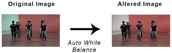
Figure 2. Example of an image before and after white balance.

In order to create the dataset alterations, we took into account the following considerations. The first relevant factor taken into account is the fact that convolutional neural networks are more sensitive to “texture“ patterns rather than the borders of a subject as shown in [14]. Additionally, as mentioned in the introduction, there are some background elements that can appear in completely different types of shots, such as trees. However giving importance only to the edges of the subjects inside an image can lead to other issues. For instance, when we have two similar types of shots, such as the half torso and the close up, the presence of certain elements (i.e., patterns) are indispensable in order to understand if a shot belongs to a class or another. Another further complication lies in the fact that some shots are difficult to classify even for humans. For instance it can be difficult to determine whether an image is a close up or an extreme close up because it shows some peculiarities of an extreme close up and some others belonging to the close up class. In light of the previous considerations, the alterations of the original dataset were decided accordingly. The first alteration of the original dataset was obtained by applying the semantic segmentation to the original dataset. Then, we used the resulting dataset. The third dataset was obtained through hypercolumns [20] extraction. Hypercolumns can be considered as pixel descriptors. They are vectors that store all the activations of every CNN unit for a certain pixel. After extracting the hypercolumns, we used them to highlight the most relevant patterns of the different images. We implemented these alterations because for the cinematographic shot classification normal data augmentation techniques can remove or alter important details. For instance if we crop a close up we end up with an extreme close up, which is a different type of shot.

Each dataset, OD, SD and HD, was then divided into training and validation sets. The train datasets(one for each image alteration) contain 7381 images, while the test sets contain 3164 images. The training datasets were used to finetune the VGG-16s, while the test sets were used to validate the models. Table 1 summarizes the datasets properties.

Table 1. Datasets’ description.

Name	Short Name	N Sample	N Sample	Alterations	Example
		Train	Test
Original	OD	7318	3164	Auto	Figure 2
Dataset				White-Balance
Stylyzed	SD	7318	3164	Semantic	Figure 3
Dataset				Segmentation
Hypercolums	HD	7318	3164	Hypercolumn	Figure 4
Dataset				Projection

3.1. The Creation of the Semantic Dataset

The Semantic Dataset, from now on SD, was created by applying the semantic segmentation to the original dataset. In order to perform the semantic segmentation we used DeepLabv3 [21], a model with state of the art performances, using an approach similar to the one described in [1]. DeepLabv3 is able to recognize different classes of objects, among which the human figure. Thus, the SD focuses on the edges of the human figure and other objects. In this way, since a shot is determined by the portion of the subject in the field of view of the camera, we helped the whole model in differentiating the images thanks to the human portion highlighted by the semantic segmentation. Figure 3 shows an image before and after the semantic segmentation.

Figure 3. Example of an image alterated for the Hypercolumns Dataset.

3.2. The Creation of the Hypercolumns Dataset

The Hypercolumns Dataset, from now on HD, refers to the dataset containing the images in which were highlighted the most relevant patterns thanks to the hypercolumns extraction [20]. An hypercolumn is a vector that contains all the outputs of the layers of a CNN for a specific area of the image. Basically, we extracted the hypercolumns, and then, we projected them on the image. The hypercolumns were extracted using a VGG-16 model pre-trained on ImageNet. These patterns were relevant because some of the classes considered have a similar aspect. For instance an half torso and an extreme close-up share some patterns, such as eyes, noses, hair texture and so on. However, other patterns show up in the half torso and not in an extreme close-up. Therefore, by extracting and projecting the hypercolumns we wanted to help the whole model to distinguish between them as much as possible. Figure 4 shows an image before and after the hypercolumns projection.

Figure 4. Example of an image alterated for the Stylized Dataset.

3.3. Image Properties and Proportion between the Different Classes

Each image used for this study had a resolution of 160 × 90 pixels. This means that the number of features for each image was equal to 14,400. This number has to be multiplied by 3, which is the number of channels used, i.e., the classic RGB configuration, for a total of 43,200 features. These properties are common to every image, regardless of the image typology. Of the before mentioned 10,545 images, 70% of them was used to train the models, while the remaining 30% was used to test them. The distribution of the images among the different classes is as follows: 1358 long shots (12.88%), 1270 medium shots (12.04%), 1080 full figures (10.24%), 935 american shots (8.87%), 1315 half figures (12.47%), 1673 half torsos (15.87%), 1731 close ups (16.41%), and 1183 extreme close ups (11.22%). The proportion among the different classes was kept between the training set and the test set.

4. Methodology

The proposed methodology relies on a two-stage classification task based on three parallel VGG-16 models using three different representations of the dataset (original, stylized and hypercolumns) and a stacking learning strategy to correctly classify different classes of movie shots. In the first classification phase, the VGG-16 models predict a class for a new sample based on what they learned during the training phase. Each network makes a prediction for a different representation of the image (original, stylized, and hypercolumns). In the second phase, the stacking-learning strategy is used. The predictions from the three VGG-16s go into a multilayer perceptron classifier, the meta-learner, which recombines them and makes a final prediction. Since our datasets were not large enough to train the VGG-16s from the beginning, we fine-tuned three different VGG-16 models, one for each typology of image, as shown by Figure 5.

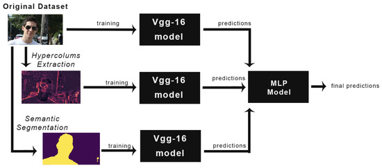
Figure 5. Methodology Overview.

A VGG-16 is a convolutional neural network developed by Visual Geometry Group based in Oxford University [22]. A Convolutional Neural Network (CNN) is a neural network that exploits convolutional layers and pooling layers in order to identify patterns inside images. The deeper is the architecture of a CNN, the more complex patterns it is able to recognize. Finetuning is a technique used when you have a small dataset, like in our case. It allows to use the weights learned from a model trained on a large dataset belonging to the same domain, in our case images. The three VGG-16 models were pre-trained on ImageNet. The finetuning was conducted not only on the fully connected layers, but also to the last convolutional layers of the network. This was conducted because a cinematographic shot is different from regular images from a conceptual point of view. Usually when a CNN classifies an image of some kind the subject is only one. On the other hand since a frame is a composition of elements it is harder to classify, because the elements included in the frame, and its patterns, may change a lot from frame to frame. The first convolutional layers were not retrained because the basic patterns are common in every type of image. After finetunig the VGG-16 models, we combined their predictions using the stacking learning technique. When the predictions of different models are combined into one final prediction we are using ensemble learning. Among the different types of techniques used to combine the prediction there is the stacking learning one. It is a technique in which the predictions are combined using a classifier instead of using other methods such as majority voting or compute the numerical average of the predictions. The classifier chosen was the multilayer perceptron (MLP) because it reaches the highest performance. In Section 5, we include the results obtained using a random forest instead of a multilayer perceptron. The MLP was trained receiving as input the predictions of the VGGs on the training sets and their corresponding labels. It was then validated with in the same way, i.e., it received the predictions of the VGGs on the validation sets and then it made its own predictions.

4.1. Methodology Adaptation with a Different Classification Task

The problem addressed in this paper allows classifying cinematographic shots into eight classes. This kind of classification is more complex to address since classes may have overlapping aspects. Many works in the literature have addressed a more general problem categorizing the classification shots into fewer classes. Since our approach is more specific it can be adapted to address a more general classification task. To this aim, for every VGG-16 model, i.e., for every model trained on a different image representation, it is sufficient to substitute the last fully connected layer of the VGG-16 models with a fully connected layer that has as many outputs as the number of classes considered. In this way, the knowledge gained by the other layers of the networks from previous training can be integrated in the fine-tuning phase. The fine-tuning phase allows the models to map the features extracted by the convolutional layers to new classes. From an architectural point of view, the difference between these new models and those represented by Figure 6 lies in the output layer. Here, the number of units has been changed from eight, the previous number of classes considered, to three, the new number of classes considered. After this phase a new meta-learner must be trained in order to perform the stacking learning strategy according to the procedure described in Section 4. Section 5.4 shows the result of our methodology on a subset of the Cinescale dataset [23].

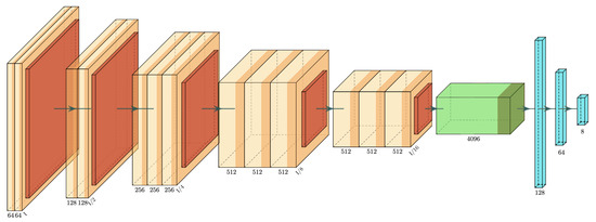
Figure 6. VGG-16 structure: the orange blocks represent the convolutional layers, the red ones are the pooling layers. The green block represents the flatten layer. Finally the blue blocks represents the fully connected layers.

4.2. Technical Details

The VGG-16 model finetuned had the following structure, shown in Figure 6. The convolutional layers were kept identical to the original architecture. The first four layers of the VGGs were not altered while the other convolutional layers were retrained. As for the fully connected layers we reduced the number of nodes in each layer passing from two fully connected layers with 4096 neurons to two fully connected layers with 128 nodes and 64 nodes. Finally the number of nodes in the output layer were reduced from the original value of 1000, the number of classes of the ImageNet dataset, to 8, the number of shots considered in this work. As for the MLP used to combine the predictions it had 3 fully connected layers. The first layer has 64 nodes, the second one 32 and the final one 8. Some of the simulations were runned with a Macbook Pro with the M1 processor. The code used for the simulation is python and the libraries used to perform the simulations and obtain the pretrained models were Keras, Tensorflow, Scikit-learn and Numpy.

5. Experimental Results

Each finetuned model has reached different performances on its own dataset. The three models were trained on 70% of the available data and tested on the remaining 30%. As previously mentioned the proportion among the different classes was maintained in order to prevent alterations in the performances. Each model was trained for 20 epochs and had a batch size of 5. The optimizer used was the stochastic gradient descent. The loss function used was the categorical crossentropy.

The model trained on the OD dataset, from now on O-VGG-16, reached a training accuracy of 97.27% and a validation accuracy of 74.27%. As for the loss function values it reached a training loss of 168,648 and a validation loss of 178,421. The model trained on the HD, from now on H-VGG-16, reached a training accuracy of 97.09% and a validation accuracy of 69.5%. As for the loss function values it reached a training loss of 169,263 and a validation loss of 181,727. Finally the model trained on the SD dataset, from now on S-VGG-16, reached a training accuracy of 94.42% and a validation accuracy of 69.41%. As for the loss function values it reached a training loss of 171,193 and a validation loss of 181,894. Table 2 refers to the confusion matrix of the O-VGG-16, while Table 3 and Table 4 refer to the S-VGG-16 and H-VGG-16 confusion matrices, respectively.

Table 2. Confusion Matrix of a VGG-16 trained on the Original Dataset.

				Predicted Labels
		LS	MS	FF	AS	HF	HT	CU	ECU
True	Long Shot (LS)	301	61	7	2	6	13	7	10
	Medium Shot (MS)	29	255	57	13	12	11	1	3
	Full Figure (FF)	1	27	252	26	4	8	2	4
Label	American Shot (AS)	0	5	26	192	52	7	0	0
	Half Figure (HF)	0	3	3	54	256	73	2	2
	Half Torso (HT)	0	6	4	1	28	435	27	2
	Close Up (CU)	0	2	1	2	1	108	376	29
	Extreme Close Up (ECU)	0	1	1	0	1	3	66	283

Table 3. Confusion Matrix of the VGG-16 trained on Stylized Dataset.

				Predicted Labels
		LS	MS	FF	AS	HF	HT	CU	ECU
True	Long Shot (LS)	331	49	3	2	0	11	8	3
	Medium Shot (MS)	41	254	52	10	7	7	9	1
	Full Figure (FF)	13	37	221	31	6	11	3	2
Label	American Shot (AS)	3	9	16	187	55	6	6	0
	Half Figure (HF)	11	9	4	37	255	62	11	4
	Half Torso (HT)	13	9	4	3	46	341	83	4
	Close Up (CU)	10	10	2	9	5	73	356	54
	Extreme Close Up (ECU)	5	3	1	2	1	10	82	251

Table 4. Confusion Matrix of a VGG-16 trained on the Hyper Dataset.

				Predicted Labels
		LS	MS	FF	AS	HF	HT	CU	ECU
True	Long Shot (LS)	312	63	20	0	7	1	2	2
	Medium Shot (MS)	48	251	56	11	11	0	2	2
	Full Figure (FF)	8	43	238	12	16	1	2	4
Label	American Shot (AS)	3	15	49	142	67	3	2	1
	Half Figure (HF)	2	15	20	38	277	34	1	6
	Half Torso (HT)	8	7	20	5	92	235	44	2
	Close Up (CU)	8	9	9	1	5	68	375	44
	Extreme Close Up (ECU)	5	0	1	1	3	5	61	279

In order to train the fourth classifier we used as data the predictions of the three VGG-16 on their training sets. After obtaining those predictions we combined those predictions by concatenating them, while also making sure that each prediction of each model was referred to the same image or its corresponding alteration. In order to validate the results, we used the same procedure. We used the predictions of the different VGG-16 models obtained from the test sets and, after concatenating them, we used those predictions to create the test set for the fourth classifier. The fourth classifier reached a training accuracy of 95.66% and a validation accuracy of 77.02%. As for the loss function values it reached a training loss of 0.2686 and a validation loss of 14,848. The confusion matrix of the fourth classifier is reported in Table 5, while Table 6 shows the performance of the fourth classifier using precision recall and f1-score.

Table 5. Confusion Matrix of the MLP as fourth classifier.

				Predicted Labels
		LS	MS	FF	AS	HF	HT	CU	ECU
True	Long Shot (LS)	320	67	3	1	4	6	4	2
	Medium Shot (MS)	30	294	36	9	7	3	1	1
	Full Figure (FF)	4	36	247	23	4	4	2	4
Label	American Shot (AS)	0	7	18	194	57	5	1	0
	Half Figure (HF)	0	6	3	44	291	44	2	3
	Half Torso (HT)	2	6	6	0	51	402	36	0
	Close Up (CU)	1	6	1	1	3	75	409	23
	Extreme Close Up (ECU)	1	0	0	0	3	3	66	282

Table 6. Precision recall and f1-score of the MLP as fourth classifier.

Labels	Precision	Recall	f1-Score	Support
Long Shot (LS)	89%	79%	84%	407
Medium Shot (MS)	70%	77%	73%	381
Full Figure (FF)	79%	76%	77%	324
American Shot (AS)	71%	69%	70%	282
Half Figure (HF)	69%	74%	72%	393
Half Torso (HT)	74%	80%	77%	503
Close Up (CU)	79%	79%	79%	519
Extreme Close Up (ECU)	90%	79%	84%	355
accuracy			77%	3164
macro avg	78%	77%	77%	3164
weighted avg	78%	77%	77%	3164

5.1. Comparisons

We tested our approach in different ways. We will show first how it performs against VGG-16 and ResNet-50 models trained with data augmentation techniques. Then, there is the comparison between our methodology and variations of the stacking learning technique. Compared to our previous work [11], there are several improvements. Previously we were able to classify only four classes, while now we are up to eight. Our previous methodology had an overall accuracy of 81.3%, while now it is a little lower; however, we are considering twice the number of classes. In addition, the dataset size has increased. Furthermore before there was no use of the stacking learning technique, we had only a VGG-16 model.

5.2. Comparison with VGG-16 and ResNet-50 Trained with Data Augmentation Techniques

We included this comparison because the ResNet-50 and the VGG-16 are the standard models to address the cinematographic shot classification [1,2]. The comparison with the VGG-16 shows that our methodology achieves better results without relying on traditional data augmentation techniques. The comparison with the ResNet-50 justify our choice to use VGG-16 architecture. Table 7 shows the different performance obtained in terms of f1-score per class and overall accuracy. The number next to the model name indicates which data augmentation techniques have been used on the dataset:

Table 7. Comparison with VGG-16 and ResNet-50.

				Predicted Labels
Model			f1	Score	per	Class			Accuracy
	LS	MS	FF	AS	HF	HT	CU	ECU
VGG-16 0	82%	69%	75%	67%	68%	75%	75%	82%	74.26%
VGG-16 1	86%	69%	77%	69%	69%	71%	79%	83%	76.55%
VGG-16 2	85%	70%	77%	72%	72%	76%	76%	85%	76.74%
VGG-16 3	85%	72%	71%	62%	69%	74%	77%	80%	74.68%
ResNet-50 1	78%	62%	61%	52%	68%	74%	71%	83%	69.15%
Us	84%	73%	77%	70%	72%	77%	79%	84%	77.09%

• Scenario 0: No data augmentation techniques used. The dataset size is its original size.
• Scenario 1: Flip images on the y-axis. The dataset size is twice the original size.
• Scenario 2: Flip images on the y-axis +zoom range = 0.1. The dataset size is three times bigger than the original size.
• Scenario 3: Flip images on the y-axis +zoom range = 0.3. The dataset size is three times bigger than the original size.

All the data augmentation techniques have been applied on the Original Dataset. Table 8 and Table 9 shows the confusion matrix and performance in terms of precision recall and f1-score, respectively, for A VGG-16 trained in Scenario 1.

Table 8. Confusion Matrix of a VGG-16 trained on the augmented Original Dataset with the flip on the y-axis, i.e., Scenario 1.

				Predicted Labels
		LS	MS	FF	AS	HF	HT	CU	ECU
True	Long Shot (LS)	375	14	3	0	2	2	4	7
	Medium Shot (MS)	71	224	56	10	8	6	1	5
	Full Figure (FF)	7	22	253	24	4	5	2	7
Label	American Shot (AS)	3	5	19	200	52	1	1	1
	Half Figure (HF)	2	4	1	57	291	31	5	2
	Half Torso (HT)	5	1	5	6	70	353	58	5
	Close Up (CU)	3	1	0	0	0	47	416	52
	Extreme Close Up (ECU)	0	1	0	0	0	0	44	310

Table 9. Precision recall and f1-score of a VGG-16 trained on the augmented Original Dataset with the flip on the y-axis, i.e., Scenario 1.

Labels	Precision	Recall	f1-Score	Support
Long Shot (LS)	80%	92%	86%	407
Medium Shot (MS)	82%	59%	69%	381
Full Figure (FF)	75%	78%	77%	324
American Shot (AS)	67%	71%	69%	282
Half Figure (HF)	68%	74%	71%	393
Half Torso (HT)	79%	70%	74%	503
Close Up (CU)	78%	80%	79%	519
Extreme Close Up (ECU)	80%	87%	83%	355
accuracy			77%	3164
macro avg	76%	76%	76%	3164
weighted avg	77%	77%	76%	3164

Table 10 and Table 11 shows the confusion matrix and performance in terms of precision recall and f1-score, respectively, for A VGG-16 trained in Scenario 2. For the performances of a VGG-16 trained in Scenario 3 consult Table 12 and Table 13. The difference between Scenario 2 and 3 lies in the magnitude of the zoom implemented. The zoom technique selects a portion of the image and rescales it. The performance of the VGG-16 trained in Scenario 0 is there a baseline. The VGG trained in Scenario 1 performs generally better than the original model, as it should, with the exception of the classifications of the half-torso class, on which it reaches a slightly lower f1-score. Moving on to Scenario 2, we can see that among the different scenarios concerning traditional data augmentation techniques the VGG-16 here reaches the best performances. However, considering that compared to the Scenario 1 Scenario 2 has training set with twice the number of samples, these performances are not too impressive. This is probably due to a phenomenon that in Scenario 3 is even more evident. Scenario 3 shows that if we increase the zoom range the performance of the model starts to drop. Such performance is related to the fact that if we zoom too much on an image belonging to a class, the resulting image belongs to another class. For instance if we zoom too much on a full figure it becomes an american shot. Finally Table 14 and Table 15 shows the confusion matrix and performance in terms of precision recall and f1-score, respectively, for a ResNet-50 trained in Scenario 2. As shown in Table 7 this model reaches the worst performance. On the other hand our proposed methodology achieves the best performance on most classes and when it is outperformed the margin is thin. The fact that it reaches performance comparable, if not superior, to those obtained with data augmentation proves its effectiveness. Additionally, in the future it can be implemented with some data augmentation techniques, such as the flip on the y-axis, in order to obtain even better performance.

Table 10. Confusion Matrix of a VGG-16 trained on the augmented Original Dataset with the flip on the y-axis and zoom range = 0.1, i.e., Scenario 2.

				Predicted Labels
		LS	MS	FF	AS	HF	HT	CU	ECU
True	Long Shot (LS)	349	51	3	1	1	0	2	0
	Medium Shot (MS)	41	272	51	7	3	7	0	0
	Full Figure (FF)	2	36	262	13	4	4	2	1
Label	American Shot (AS)	2	7	25	201	43	3	0	1
	Half Figure (HF)	4	8	9	51	278	41	1	1
	Half Torso (HT)	5	9	5	3	50	408	23	0
	Close Up (CU)	6	5	2	3	3	97	361	42
	Extreme Close Up (ECU)	3	3	0	0	1	4	47	297

Table 11. Precision recall and f1-score of a VGG-16 trained on the augmented Original Dataset with the flip on the y-axis and zoom range = 0.1, i.e., Scenario 2.

Labels	Precision	Recall	f1-Score	Support
Long Shot (LS)	85%	86%	85%	407
Medium Shot (MS)	70%	71%	70%	381
Full Figure (FF)	73%	81%	77%	324
American Shot (AS)	72%	71%	72%	282
Half Figure (HF)	73%	71%	72%	393
Half Torso (HT)	72%	81%	76%	503
Close Up (CU)	83%	70%	76%	519
Extreme Close Up (ECU)	87%	84%	85%	355
accuracy			77%	3164
macro avg	77%	77%	77%	3164
weighted avg	77%	77%	77%	3164

Table 12. Confusion Matrix of a VGG-16 trained on the augmented Original Dataset with the flip on the y-axis and zoom range = 0.3, i.e., Scenario 3.

				Predicted Labels
		LS	MS	FF	AS	HF	HT	CU	ECU
True	Long Shot (LS)	353	29	3	4	5	3	8	2
	Medium Shot (MS)	37	266	55	9	10	3	1	0
	Full Figure (FF)	3	41	235	31	7	3	3	1
Label	American Shot (AS)	1	5	10	216	49	0	1	0
	Half Figure (HF)	1	1	2	66	288	32	3	0
	Half Torso (HT)	1	2	4	2	75	371	48	0
	Close Up (CU)	2	1	0	0	4	77	429	6
	Extreme Close Up (ECU)	1	1	0	1	0	5	126	221

Table 13. Precision recall and f1-score of a VGG-16 trained on the augmented Original Dataset with the flip on the y-axis and zoom range = 0.3, i.e., Scenario 3.

Labels	Precision	Recall	f1-Score	Support
Long Shot (LS)	88%	87%	88%	407
Medium Shot (MS)	77%	70%	73%	381
Full Figure (FF)	76%	73%	74%	324
American Shot (AS)	66%	77%	71%	282
Half Figure (HF)	66%	73%	69%	393
Half Torso (HT)	75%	74%	74%	503
Close Up (CU)	69%	83%	75%	519
Extreme Close Up (ECU)	96%	62%	76%	355
accuracy			75%	3164
macro avg	77%	75%	75%	3164
weighted avg	77%	75%	75%	3164

Table 14. Confusion Matrix of a Resnet-50 trained on OD plus flip on the y-axis.

				Predicted Labels
		LS	MS	FF	AS	HF	HT	CU	ECU
True	Long Shot (LS)	275	118	6	0	2	3	2	1
	Medium Shot (MS)	20	236	33	1	0	0	1	0
	Full Figure (FF)	2	89	218	5	5	3	1	1
Label	American Shot (AS)	1	38	90	115	36	2	0	0
	Half Figure (HF)	1	36	16	36	257	45	1	1
	Half Torso (HT)	1	27	13	1	53	390	18	0
	Close Up (CU)	0	23	6	3	7	109	317	54
	Extreme Close Up (ECU)	2	10	6	0	2	5	40	290

Table 15. Precision recall and f1-score of a ResNet50 trained on the OD plus the flip on the y-axis.

Labels	Precision	Recall	f1-Score	Support
Long Shot (LS)	91%	68%	78%	407
Medium Shot (MS)	49%	86%	62%	381
Full Figure (FF)	56%	67%	61%	324
American Shot (AS)	72%	41%	52%	282
Half Figure (HF)	71%	65%	68%	393
Half Torso (HT)	70%	78%	74%	503
Close Up (CU)	83%	61%	71%	519
Extreme Close Up (ECU)	84%	82%	83%	355
accuracy			69%	3164
macro avg	72%	68%	68%	3164
weighted avg	73%	69%	69%	3164

5.3. Comparison with Variations of the Stacking Learning Technique

There are already different studies that prove the benefits of stacking ensemble compared to other types of ensembles [4,17]. So we will show the performance of our approach compared to different implementations of the stacking learning strategy. Table 16 shows the different results obtained with the different stacking learning techniques. The first alteration was obtained by using a Random Forest as fourth classifier, i.e., meta-learner, instead of the MLP. In Table 17 and Table 18 are reported the results obtained while using a random forest instead of a MLP as classifier. The second alteration was obtained in the following way. Instead of training three separated VGG-16 models in addition to the fourth classifier we merged the four models into one. We called this network the Cerberus model. Like in our methodology the meta-learner is a Multilayer Perceptron. Instead of having four different models, here, we have only one network with three “heads“, one for each dataset. The confusion matrix for the Cerberus model and additional metrics are reported in Table 19 and Table 20, respectively. The results show that our approach has a better performance compared to those obtained with different alterations of the stacking learning. Table 21 summarizes all the comparisons conducted.

Table 16. Comparison with Variation of the Stacking Learning Technique.

Model			f1	Score	per	Class			Accuracy
		LS	MS	FF	AS	HF	HT	CU	ECU
Random Forest	65%	70%	76%	71%	72%	76%	79%	83%	72.56%
as meta-learner
Us: MLP	84%	73%	77%	70%	72%	77%	79%	84%	77.09%
as meta-learner
Cerberus	83%	71%	68%	66%	63%	75%	73%	83%	73.32%

Table 17. Confusion Matrix of random forest trained on predictions.

				Predicted Labels
		LS	MS	FF	AS	HF	HT	CU	ECU
True	Long Shot (LS)	375	30	1	0	1	0	0	0
	Medium Shot (MS)	106	244	29	0	1	0	0	1
	Full Figure (FF)	53	25	224	15	3	3	0	1
Label	American Shot (AS)	49	2	11	177	42	0	0	1
	Half Figure (HF)	54	4	2	26	271	34	1	1
	Half Torso (HT)	48	5	2	1	46	359	42	0
	Close Up (CU)	36	3	0	1	0	49	403	27
	Extreme Close Up (ECU)	25	0	0	0	0	0	55	275

Table 18. Precision recall and f1-score of a random forest on the predictions of the three vgg-16.

Labels	Precision	Recall	f1-Score	Support
Long Shot (LS)	50%	92%	65%	407
Medium Shot (MS)	78%	64%	70%	381
Full Figure (FF)	83%	69%	76%	324
American Shot (AS)	80%	63%	71%	282
Half Figure (HF)	74%	69%	72%	393
Half Torso (HT)	81%	71%	76%	503
Close Up (CU)	80%	78%	79%	519
Extreme Close Up (ECU)	90%	77%	83%	355
accuracy			74%	3164
macro avg	77%	73%	74%	3164
weighted avg	77%	74%	74%	3164

Table 19. Confusion Matrix of the cerberus model VGG-16 trained on the three Datasets.

		LS	MS	FF	AS	HF	HT	CU	ECU
True	Long Shot (LS)	317	80	6	1	2	1	0	0
	Medium Shot (MS)	27	304	35	6	5	3	0	1
	Full Figure (FF)	4	54	212	38	6	7	2	1
Label	American Shot (AS)	0	11	29	203	37	2	0	0
	Half Figure (HF)	2	6	7	79	221	75	2	1
	Half Torso (HT)	1	12	8	4	36	418	23	1
	Close Up (CU)	4	10	4	6	3	107	337	48
	Extreme Close Up (ECU)	1	4	2	0	0	4	36	308

Table 20. Precision recall and f1-score of the Cerberus model trained on the three datasets.

Labels	Precision	Recall	f1-Score	Support
Long Shot (LS)	89%	78%	83%	407
Medium Shot (MS)	63%	80%	71%	381
Full Figure (FF)	70%	65%	68%	324
American Shot (AS)	60%	72%	66%	282
Half Figure (HF)	71%	56%	63%	393
Half Torso (HT)	68%	83%	75%	503
Close Up (CU)	84%	65%	73%	519
Extreme Close Up (ECU)	86%	87%	86%	355
accuracy			73%	3164
macro avg	74%	73%	73%	3164
weighted avg	75%	73%	73%	3164

Table 21. f1-score per class and accuracy of different architectures.

				Models’ f1-Score per Class
Models	Ovgg-16	Ovgg	Ovgg	Ovgg	MLP	Cerberus	ResNet	Random
		aug1	aug2	aug3			50	Forest
Classes
LS	82%	86%	85%	85%	84%	83%	78%	65%
MS	69%	69%	70%	72%	73%	71%	62%	70%
FF	75%	77%	77%	71%	77%	68%	61%	76%
AS	67%	69%	72%	62%	70%	66%	52%	71%
HF	68%	71%	72%	69%	72%	63%	68%	72%
HT	75%	74%	76%	74%	77%	75%	74%	76%
CU	75%	79%	76%	77%	79%	73%	71%	79%
ECU	82%	83%	85%	80%	84%	86%	83%	83%
Acc	74.27%	76.55%	76.74%	74.68%	77.09%	73.32%	69.15%	72.56%

5.4. Performance of Our Approach Adapted to a Real Dataset with Three Classes

We adapted the methodology described in Section 4 to a real dataset. To perform the model adaptation and evaluation, we used a subset of the Cinescale dataset. This dataset has 9 classes regrouped into 3 macro-classes of shots: long shots, medium shots and close ups. To obtain a dataset with three classes we followed the partition illustrated in [23]. The Cinescale subset was divided into a train set and a test set. The train set has 12,597 images, which were used to fine-tune our models, while the test set has 5553 images, which were used to evaluate our two-stage classification methodology. By taking a look at Table 22, that shows our performance in terms of precision, recall and f-1 score, we can see that our methodology performs well in terms of precision. In terms of recall, we can see that our approach achieves a better performance on the medium shots (96%) than with the long shots (66%) and close ups (65%). These lower scores can be explained with the high unbalance of the dataset. In fact, the medium shots compose the 78% of the dataset, while long shots and close ups amount to 6% and 16%, respectively. If we take a look at the confusion matrix reported in Table 23, we can see that most of the misclassified samples are medium shots classified as long shots and close ups and vice versa. Due to the high unbalance of the dataset it is not surprising that there is a bias towards the prediction of medium shots. On the other hand, the amount of close ups wrongly labeled as long shots and vice versa is very low, with 8 long shots classified as close ups and 5 close ups classified as long shots. Overall, our methodology was able to reach an weighted accuracy of 89%, as reported in Table 22.

Table 22. Precision recall and f1-score of our methodology on a subset of the Cinescale Dataset.

Labels	Precision	Recall	f1-Score	Support
Long Shot (LS)	81%	66%	73%	345
Medium Shot (MS)	91%	96%	93%	4345
Close Up (CU)	79%	65%	71%	863
accuracy			89%	5553
macro avg	84%	75%	79%	5553
weighted avg	89%	89%	89%	5553

Table 23. Confusion Matrix of our methodology on a subset of the Cinescale dataset.

		Predicted Labels
		LS	MS	CU
True	Long Shot (LS)	226	111	8
	Medium Shot (MS)	141	4175	47
Labels	Close Up (CU)	5	295	563

6. Conclusions and Future Research Direction

The proposed approach shows good results. Our two-stage classification methodology implementing the stacking learning strategy overall performs better by a small margin than traditional approaches and reaches an accuracy of 77%. Furthermore, in order to obtain even better performances our approach can be integrated with data augmentation techniques such as the flip on the y-axis. In a preliminary experiment, we combined our approach with the data augmentation techniques of Scenario 2. In this case, the three VGG-16 were trained using the data augmentation techniques proposed in Scenario 2 and then the resulting predictions on the training sets were used to train the MLP classifier. The results reported in Table 24 and Table 25 refer to the same test set used so far. The resulting accuracy rises to 78%. This shows that the task at hand is difficult. It also shows that it is possible to integrate the proposed approach with traditional data augmentation techniques. There is a further consideration to make. As previously mentioned in the introduction there is a certain amount of samples that can fall in different classes since they show properties of both classes. Thus, while an accuracy of 78% is good, although far from ideal, the actual performance of an implemented model should be higher in the eyes of a user. This is because the majority of the misclassification errors are made on those samples that fall between two classes. Its main drawback is that, since it requires the intervention of different deep neural networks, it cannot be used for real time events; however, it is able to classify 8 different classes of cinematographic shot classification. As shown by the confusion matrix in Table 25, the mistakes made are between classes very similar to each other. There are still improvements that could be made. The number of classes is sufficient however it would be interesting to extend the approach in order to define if a scene is indoor or outdoor. Then, another interesting integration could be to extend the approach to videos in order to also classify camera movements, instead of only the camera field of view.

Table 24. Precision recall and f1-score of a mlp as fourth classifier trained on the predictions of three VGG-16 trained on each dataset with data augmentation techniques.

Labels	Precision	Recall	f1-Score	Support
Long Shot (LS)	87%	85%	86%	407
Medium Shot (MS)	72%	76%	74%	381
Full Figure (FF)	76%	81%	79%	324
American Shot (AS)	76%	73%	75%	282
Half Figure (HF)	71%	73%	72%	393
Half Torso (HT)	77%	75%	76%	503
Close Up (CU)	76%	80%	78%	519
Extreme Close Up (ECU)	91%	81%	86%	355
accuracy			78%	3164
macro avg	78%	78%	78%	3164
weighted avg	78%	78%	78%	3164

Table 25. Confusion matrix of a mlp as fourth classifier trained on the predictions of three VGG-16 trained on each dataset with data augmentation techniques.

				Predicted Labels
		LS	MS	FF	AS	HF	HT	CU	ECU
True	Long Shot (LS)	346	50	4	0	2	0	3	2
	Medium Shot (MS)	35	289	46	6	2	3	0	0
	Full Figure (FF)	4	35	263	11	6	2	3	0
Label	American Shot (AS)	2	6	22	206	43	0	3	0
	Half Figure (HF)	1	7	7	46	287	37	8	0
	Half Torso (HT)	6	9	3	1	57	375	52	0
	Close Up (CU)	2	4	1	0	6	64	414	28
	Extreme Close Up (ECU)	0	1	0	0	2	3	60	289

References

- Bak, H.Y.; Park, S.B. Comparative Study of Movie Shot Classification Based on Semantic Segmentation. Appl. Sci. 2020, 10, 3390. [Google Scholar] [CrossRef]
- Savardi, M.; Signoroni, A.; Migliorati, P.; Benini, S. Shot scale analysis in movies by convolutional neural networks. In Proceedings of the 2018 25th IEEE International Conference on Image Processing (ICIP), Athens, Greece, 7–10 October 2018; pp. 2620–2624. [Google Scholar] [CrossRef]
- Svanera, M.; Savardi, M.; Signoroni, A.; Kovács, A.B.; Benini, S. Who is the Film’s Director? Authorship Recognition Based on Shot Features. IEEE MultiMedia 2019, 26, 43–54. [Google Scholar] [CrossRef]
- Odegua, R. An empirical study of ensemble techniques. In Proceedings of the International Conference on Deep Learning IndabaXAt, Bangkok, Thailand, 13–15 December 2019. [Google Scholar]
- Canini, L.; Benini, S.; Leonardi, R. Classifying cinematographic shot types. Multimed. Tools Appl. 2011, 62, 51–73. [Google Scholar] [CrossRef]
- Svanera, M.; Benini, S.; Adami, N.; Leonardi, R.; Kovács, A.B. Over-the-shoulder shot detection in art films. In Proceedings of the 2015 13th International Workshop on Content-Based Multimedia Indexing (CBMI), Prague, Czech Republic, 10–12 June 2015; pp. 1–6. [Google Scholar]
- Cherif, I.; Solachidis, V.; Pitas, I. Shot type identification of movie content. In Proceedings of the 2007 9th International Symposium on Signal Processing and Its Applications, Sharjah, UAE, 12–15 February 2007; pp. 1–4. [Google Scholar]
- Hasan, M.A.; Xu, M.; He, X.; Xu, C. CAMHID: Camera Motion Histogram Descriptor and Its Application to Cinematographic Shot Classification. IEEE Trans. Circuits Syst. Video Technol. 2014, 24, 1682–1695. [Google Scholar] [CrossRef]
- Wang, H.L.; Cheong, L. Taxonomy of Directing Semantics for Film Shot Classification. IEEE Trans. Circuits Syst. Video Technol. 2009, 19, 1529–1542. [Google Scholar] [CrossRef]
- Bhattacharya, S.; Mehran, R.; Sukthankar, R.; Shah, M. Classification of Cinematographic Shots Using Lie Algebra and its Application to Complex Event Recognition. IEEE Trans. Multimed. 2014, 16, 686–696. [Google Scholar] [CrossRef][Green Version]
- Vacchetti, B.; Cerquitelli, T.; Antonino, R. Cinematographic shot classification through deep learning. In Proceedings of the 2020 IEEE 44th Annual Computers, Software, and Applications Conference (COMPSAC), Madrid, Spain, 13–17 July 2020; pp. 345–350. [Google Scholar] [CrossRef]
- Rao, A.; Wang, J.; Xu, L.; Jiang, X.; Huang, Q.; Zhou, B.; Lin, D. A unified framework for shot type classification based on subject centric lens. In Computer Vision—ECCV 2020; Vedaldi, A., Bischof, H., Brox, T., Frahm, J.M., Eds.; Springer International Publishing: Cham, Switzerland, 2020; pp. 17–34. [Google Scholar]
- Tan, C.; Sun, F.; Kong, T.; Zhang, W.; Yang, C.; Liu, C. A survey on deep transfer learning. In Proceedings of the 27th International Conference on Artificial Neural Networks, Rhodes, Greece, 4–7 October 2018; pp. 270–279. [Google Scholar] [CrossRef]
- Geirhos, R.; Rubisch, P.; Michaelis, C.; Bethge, M.; Wichmann, F.A.; Brendel, W. ImageNet-trained CNNs are biased towards texture; increasing shape bias improves accuracy and robustness. arXiv 2018, arXiv:1811.12231. [Google Scholar]
- Huang, Q.; Xiong, Y.; Rao, A.; Wang, J.; Lin, D. MovieNet: A Holistic Dataset for Movie Understanding. In Computer Vision—ECCV 2020; Vedaldi, A., Bischof, H., Brox, T., Frahm, J.M., Eds.; Springer International Publishing: Cham, Switzerland, 2020; pp. 709–727. [Google Scholar]
- Logan, R.; Williams, B.G.; Ferreira da Silva, M.; Indani, A.; Schcolnicov, N.; Ganguly, A.; Miller, S.J. Deep Convolutional Neural Networks With Ensemble Learning and Generative Adversarial Networks for Alzheimer’s Disease Image Data Classification. Front. Aging Neurosci. 2021, 13, 720226. [Google Scholar] [CrossRef] [PubMed]
- Yazdizadeh, A.; Patterson, Z.; Farooq, B. Ensemble Convolutional Neural Networks for Mode Inference in Smartphone Travel Survey. IEEE Trans. Intell. Transp. Syst. 2020, 21, 2232–2239. [Google Scholar] [CrossRef]
- Andriluka, M.; Pishchulin, L.; Gehler, P.; Schiele, B. 2D human pose estimation: New benchmark and state of the art analysis. In Proceedings of the IEEE Conference on Computer Vision and Pattern Recognition (CVPR), Columbus, OH, USA, 23–28 June 2014. [Google Scholar]
- Huang, G.B.; Ramesh, M.; Berg, T.; Learned-Miller, E. Labeled Faces in the Wild: A Database for Studying Face Recognition in Unconstrained Environments; Technical Report; University of Massachusetts: Amherst, MA, USA, 2007. [Google Scholar]
- Hariharan, B.; Arbelaez, P.; Girshick, R.; Malik, J. Hypercolumns for Object Segmentation and Fine-grained Localization. In Proceedings of the IEEE Conference on Computer Vision and Pattern Recognition, Boston, MA, USA, 7–12 June 2015; pp. 447–456. [Google Scholar]
- Chen, L.C.; Papandreou, G.; Schroff, F.; Adam, H. Rethinking Atrous Convolution for Semantic Image Segmentation. arXiv 2017, arXiv:abs/1706.05587. [Google Scholar]
- Simonyan, K.; Zisserman, A. Very deep convolutional networks for large-scale image recognition. In Proceedings of the 3rd International Conference on Learning Representations, ICLR 2015, San Diego, CA, USA, 7–9 May 2015; Bengio, Y., LeCun, Y., Eds.; OpenReview: San Diego, CA, USA, 2015. [Google Scholar]
- Savardi, M.; Kovács, A.B.; Signoroni, A.; Benini, S. CineScale: A dataset of cinematic shot scale in movies. Data Brief 2021, 36, 107002. [Google Scholar] [CrossRef] [PubMed]
Publisher’s Note: MDPI stays neutral with regard to jurisdictional claims in published maps and institutional affiliations. |
© 2022 by the authors. Licensee MDPI, Basel, Switzerland. This article is an open access article distributed under the terms and conditions of the Creative Commons Attribution (CC BY) license (https://creativecommons.org/licenses/by/4.0/).