A Saliency-Based Patch Sampling Approach for Deep Artistic Media Recognition

Abstract

We present a saliency-based patch sampling strategy for recognizing artistic media from artwork images using a deep media recognition model, which is composed of several deep convolutional neural network-based recognition modules. The decisions from the individual modules are merged into the final decision of the model. To sample a suitable patch for the input of the module, we devise a strategy that samples patches with high probabilities of containing distinctive media stroke patterns for artistic media without distortion, as media stroke patterns are key for media recognition. We design this strategy by collecting human-selected ground truth patches and analyzing the distribution of the saliency values of the patches. From this analysis, we build a strategy that samples patches that have a high probability of containing media stroke patterns. We prove that our strategy shows best performance among the existing patch sampling strategies and that our strategy shows a consistent recognition and confusion pattern with the existing strategies.

1. Introduction

The rapid progress of deep learning techniques addresses many challenges in computer vision and graphics. For example, styles learned from examplar artwork images is applied to style input photographs. In many applications, generation comes from recognition. In the studies that generate styles on input photographs, the style is implicitly recognized in the form of texture-based feature maps. The explicit recognition of a style is still a challenging problem.

Style has various components such as school, creator, age, mood and artistic media. Among the various components, we concentrate on artistic media used to express the style. The texture of distinctive stroke patterns from the artistic medium such as pencil, oilpaint brush or watercolor brush is the key to recognize the artistic medium. In many studies, the features extracted using classical object recognition techniques are employed to recognize and classify the artistic media.

Many models that recognize artistic media from artwork images are devised based on deep neural network models that show convincing performance in recognizing and classifying objects. The preliminary media recognizing models process the whole artwork image for the recognition. Some recent models process a series of patches sampled from the artwork image to improve the accuracy of recognition. This improvement comes from the point that the stroke patterns, which are prominent evidence of an artistic medium, locate in a local scale. Therefore, a patch that successively catches this stroke pattern shows higher accuracy. However, since such patches are hard to sample properly, the patch-based models cannot show consistent accuracies. A scheme that samples patches capturing stroke patterns from an artwork image in a high probability can improve the accuracy of a media recognition technique.

We devise a patch sampling strategy by observing how humans recognize artistic media from an artwork image. Humans tend to concentrate on the stroke patterns on an artwork to recognize the media by ignoring other aspects of the artwork. We build a saliency-based approach to mimic such a concentration. Saliency is defined as a quantized measurement of distinctiveness of a pixel. We estimate a distribution of saliency scores of the patches sampled from an artwork image. Then, we build a relation between the distribution and the human-concentrated patch by executing a human study. Finally, we build a strategy to sample a patch that catches the distinctive stroke patterns based on saliency and apply this strategy to improve the accuracy of the existing media recognition models.

Our strategy begins by estimating saliency values from an artwork image. To find the saliency values that correspond to the stroke patterns of the image, we execute a human study. We hire mechanical turks to manually mark the regions of prominent stroke patterns in an artwork image. The saliency values on the pixels those belong to these regions are estimated to build a strategy for selecting the regions automatically.

The remainder of this paper is structured as follows. In Section 2, we survey related works that recognize artistic style and media, while in Section 3 we propose our saliency-based patch sampling strategy. In Section 4, we present our multi-column structured framework and in Section 5, we measure the accuracy of our framework. We compare it with that of existing recognizers and analyze the results in Section 6. Finally, we conclude our proposed approach and suggest proposals for future work in Section 7.

2. Related Works

Researchers have developed various methods for recognizing different elements of artworks, such as styles, genres, objects, creators and artistic media. We classify the existing schemes according to the features they employed.

2.1. Handcrafted Features for Recognizing Style and Artist

Several researchers have presented methods combining handcrafted features and decision strategies, including SVM. Liu et al. [1] combined features including color, composition, and line, and demonstrated that this combination of features led to better performance than a CNN-based feature methods. Florea et al. [2] employed features such as color structure and topographical features and exploited SVG as their decision method. Their scheme exhibited better performance than deep CNN structures such as ResNet-34. However, these handcrafted feature-based methods are no longer commonly studied, as the performance of CNNs has dramatically improved.

Recently, Liao et al. [3] presented an oil painter recognition model based on traditional cluster multiple kernel learning algorithm working on various handcrafted features. Their features include both global features such as color LBP, color GIST, color PHOG, CIE, Canny edges, and local features such as complete LBP, color SIFT, and SSIM. The accuracy for recognition ranges in 0. 512∼0.546 according to their algorithms.

2.2. CNN-Based Features for Recognizing Style and Artist

2.2.1. Fusioned Features

In early research, Karayev et al. [4] combined handcrafted features and features extracted from AlexNet, an early deep CNN model, to recognize artwork styles. As the first step, they compared features from AlexNet with various handcrafted features including L*a*b* color histogram, GIST, graph-based visual saliency, meta-class binary features and content classifier confidence. They then demonstrated that the combination of features from AlexNet and the content classifier results in the best performance in recognizing styles. Bar et al. [5] also combined features from AlexNet and PiCodes, a compact image descriptor for object category recognition, for the purpose of style recognition.

Recently, Zhong et al. [6] classified the styles of artwork images based on brush stroke information. For this purpose, they suggested gray-level co-occurrence matrix (GLCM) that detects and represents brush strokes. The information embedded in GLCM is processed through deep convolutional neural network to extract relevant feature maps, which are further processed using SVM.

2.2.2. CNN-Based Features

A number of studies have demonstrated that CNN models without additional features exhibit acceptable performance for recognizing artwork styles. Some researchers employed AlextNet with minor improvements [7,8,9], while other employed state-of-the-art CNN models, such as VGGNet and ResNet [10,11,12]. They have also extended their datasets, including WikiArt, the Web Gallery of Artworks (WGA), TICC and OmniArt, by expanding the size and increasing the variety of the datasets. The size of WikiArt has been increased by more than 133 K through incrementally collecting artwork images. The WGA is a historical artwork dataset including artworks from the 8th century to the 19th century with extensive collections of medieval and renaissance artworks. TICC is composed of digital photographic reproductions of artworks from the Rijks that have uniform color and physical size. OmniArt, a museum-centric dataset, combines several datasets from museums including the Rijks, the Metropolitan Museum of Art and the WGA.

2.2.3. Gram Matrix

In several studies, texture information plays an important role in recognizing artwork styles and synthesizing artistic styles in photographs. These studies employ the Gram matrix, which is effective for processing texture information [13]. The Gram matrix is defined as the correlation between different filter responses of CNN layers. Each element of the matrix represents the level of spatial similarity between feature responses in a layer.

In contrast to the CNN-based features, which are specialized for object recognition, Gram-based texture information is effective in improving the performance of style recognition. Sun et al. [14] demonstrated the effectiveness of the Gram matrix for style recognition by combining the features from an object-classifying CNN structure and the texture information represented in a Gram matrix. Chu et al. [15,16] employed both features from a Gram matrix and a Gram of Gram matrix for style recognition. The recognition module used in these works is VGGNet. The performance of the style recognition methods using the Gram matrix is superior to that of methods using CNN models. We compare the performance of the features from the Gram matrix with the performance of our approach and demonstrate that a multi-column structure using well preserved stroke patterns is effective for media recognition.

More recently, Chen and Yang [17] presented a style recognition framework using adaptive cross-layer correlation, which is inspired by Gram matrix. They classified artworks into 13 painting styles at 73.67% on the arc-Dataset and 80.53% on the Hipster Wars dataset.

2.2.4. Features for Fine-Grained Region

In multi-column structured models devised for image aesthetic assessment [18,19,20,21], local patches sampled from an image are fed into the recognition modules in the model. Many existing object-classifying CNN models are employed for the recognition module. Instead of carefully sampling patches, these methods focus on processing the features extracted from the recognition modules for media recognition.

Anwer et al. [22] proposed a multi-column structured model for style recognition. They sampled patches from portrait images based on prominent components such as the eyes, nose and lips. This object-based sampling strategy cannot be applied for media recognition, since most artists tend to hide stroke patterns in describing the details of salient objects. In our approach, we devise a saliency-based scheme to properly sample patches containing stroke textures.

Yang and Min [23] proposed a multi-column structure to recognize artistic media from existing artworks and to evaluate synthesized artistic media effects, which are produced by many existing technologies. They collect dataset for synthesized artistic media effects for their experiment. Through our further analysis, the media stroke textures on the artwork images play an important role in recognizing the media. Since this structure does not include any considerations on how to concentrate on the stroke textures, the performance of this structure can be improved.

Sandoval et al. [24] presented a classification approach for art paintings by feeding five patches cropped from four corners and center of the painting into a multi-layered deep CNN. They employed various well-known architectures including AlexNet, VGGNet, Goog-LeNet and ResNet to classify the art paintings into their styles. They experimented the process by designing several scenarios that specify various conditions such as voting and weight strategy. However, their approach has a limitation in considering how to crop the patch to reflect the style of the painting.

Bianco et al. [25] presented a painting classification scheme that samples ROIs from the painting for the input of multi-branch deep neural network. They present two sampling strategies: a random crop and a smart extracting scheme based on spatial transform network. They also employ various handcrafted features along with the neural ones. They classified the genre, artist and style of the paintings at the accuracy of 56.5∼63.6%.

2.3. CNN-Based Feature for Recognizing Artistic Media

Of the studies pertaining style recognition, only several focused on media recognition. In addition to style and creator, their targets for recognition include type, material, and year of creation. These methods were motivated by style recognition studies and exploited various features.

Mensink et al. [26] presented a framework that classifies artworks from the Rijks dataset according to their creators, types, materials and years of creation. They employed SIFT encoded with Fisher vector for feature extraction, and an SVM for the decision process. They aim to classify twelve materials including paper, wood, silver, oil, ink and watercolor. Their approach involves classifying materials in an artwork dataset using handcrafted features. However, the wide range of materials makes the classification a straightforward process. Furthermore, SIFT, their features for extraction, has difficulty in distinguishing the stroke patterns of similar textures. Therefore, their framework is limited in its ability to classify artistic media, which is a more complex problem.

Strezoski et al. [12] pursued the same classification problem as Mensink et al. using both the Rijks and OmniArt datasets. The most important technical improvement of their study is that it employs features extracted from CNN models instead of handcrafted features. They used several widely used CNN models including VGGNet, ResNet and Inception V2 to extract features from artwork images. The results of their experiment indicate that the features from ResNet led to the best performance. They addressed different types of recognition problems such as classification, multi-label classification and regression using a single structure. However, a single structure model of fixed size input images has the drawback of distortion caused by resizing the input images.

Mao et al. [27] extended the object of classification into content such as stories, genre, artist, medium, historical figure and event. They employed features from VGGNet and the Gram matrix for their classification. For this purpose, they constructed Art500K dataset from various sources including WikiArt, WGA, Rijks, and Google Arts and Culture. One of their important contributions is a practical implementation. They present a website and mobile application through which users can upload their artwork images to extract information. Users can also search artworks that share similar properties by filtering categories and by visual similarity. They used historical artwork datasets which are widely used in style recognition studies. However, these datasets are not appropriate for training and testing for the recognition of artistic media, because the stroke patterns of historical datasets have been damaged. While they contribute to the expansion of recognizing the target domain, they do not offer any strategies for preserving the stroke pattern.

3. Building Saliency-Based Patch Sampling Strategy from Human Study

In this section, we aim to develop a patch sampling strategy that catches the media stroke texture, which is the key evidence of recognizing media. We begin by estimating $s_i$, a saliency score of a patch $p_i$, which is defined as the mean of the saliency values of the pixels on the patch $p_i$. $s_i$’s, the saliency scores of the patches sampled from an image, are collected to build $P\left(s\right)$, a distribution of the saliency scores. In the second stage, we hire mechanical turks to watch an artwork image and to mark the region from which they catch the evidence of the artistic media that creates the artwork image they are watching. A patch containing the region is denoted as gtPatch, which means the ground truth patch for the media. The saliency scores of the gtPatches, which are denoted as $z_i$, are marked on $P\left(s\right)$, the distribution of the saliency scores. These two steps are illustrated in Figure 1. Finally, $z_i$, the saliency scores of the gtPatches marked on the distribution, are collected for the distribution of the saliency scores of gtPatches. For an arbitrary artwork image, a patch whose saliency score is the median of this distribution is expected to be a gtPatch for the image.

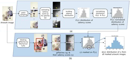
Figure 1. Two processes to build our saliency-based patch sampling scheme: (a) building the distribution of saliency scores for an input artwork image, (b) building the distribution of saliency scores for a gtPatch.

3.1. Building the Distribution of Saliency Scores of Patches

3.1.1. Review of Saliency Estimation Schemes

According to a recent survey on saliency estimation techniques [28], 751 research papers were published on this topic since 2008. Some of them employ conventional techniques including contrast, diffusion, backgroundness and objectness prior, low-rank matrix recovery, and Bayesian, etc, and others employ deep learning techniques including supervised, weakly supervised and adversarial methods. In order to select a proper saliency estimation technique for our purpose, we build the following requirements: (i) uniformly highlighting salient regions with well-defined boundaries, (ii) many salient region candidates that potentially contain media stroke texture, and (iii) a wide range of saliency values.

From these requirements, we can locate important objects in more salient regions and media stroke textures in less salient regions. Figure 2 illustrates several saliency estimation results. We exclude frequency-based methods that do not clearly distinguish objects and backgrounds. We also exclude context-aware detection schemes, since they concentrate on the edges of important objects. We select robust background detection schemes that emphasize objects in stronger saliency values. Among the various robust background detection schemes [29,30,31,32], we select Zhu et al.’s work [32] that presents an efficient computation environment.

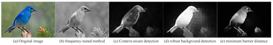
Figure 2. Results of candidate saliency estimations.

3.1.2. Efficient Computation of Saliency Score of Patches

Values in the saliency map are between zero to one (see Figure 3b). We define the saliency score of a single patch as the average of the salient values of pixels inside the patch. The patches have an identical $256\times 256$ pixel size (see Figure 3c) and the saliency scores of all patches inside an input image are computed (see Figure 3d).

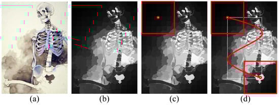
Figure 3. Process of computing the saliency score of all patches of an image. (a) input artwork image, (b) corresponding saliency map, (c) saliency score computation for a patch with a size of 256 × 256, (d) saliency score computation of all patches inside an input image.

Estimating the saliency score for a patch may require a heavy computational load, as all possible patches from an artwork image are considered. This may require a time complexity of $O(k^2\times n^2)$ for an image of $n\times n$ resolution and a patch of $k\times k$ size. Because we set k to 256, which is as large as n, $O(k^2\times n^2)$ could nearly be $O\left(n^4\right)$.

For efficient estimation, we use a cumulative summation scheme with an auxiliary memory R of size $n\times n$. $R\left(q\right)$, where $q=(i,j)$, stores the sum of the saliency values in a patch defined by O and q, where O is the origin of the image. From $s(x,y)$, the saliency values at a pixel $(x,y)$, $R(i,j)$ is computed by the following formula:

$$R(i,j)=s(i,j)+R(i-1,j)+R(i,j-1)-R(i-1,j-1).$$

(1)

This formula is implemented through the pseudocode in Figure 4 and illustrated in Figure 5c.

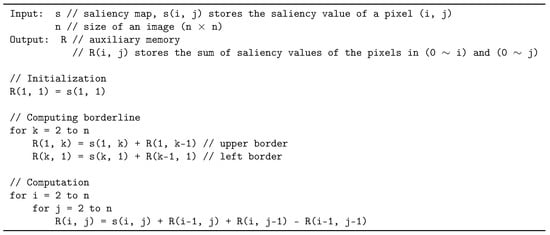
Figure 4. Pseudocode for computing auxiliary memory R from a saliency map s.

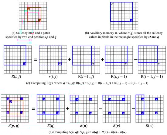
Figure 5. The process of computing auxiliary memory R and saliency score S of an image, which is motivated by cumulative sum algorithm.

The above algorithm has a time complexity of $O\left(n^2\right)$. Using R, we estimate $S(p,q)$, the saliency score of a patch defined by an upper left vertex $p=(p_x,p_y)$ and a lower right vertex $q=(q_x,q_y)$, as follows:

$$S(p,q)=R(q_x,q_y)+R(p_x,p_y)-R(q_x,p_y)-R(p_x,q_y)$$

(2)

This formula is illustrated in Figure 5d. Note that $S(p,q)$ takes $O\left(1\right)$ to be computed.

3.1.3. Building the Distribution of Saliency Scores

$s_i$, the saliency scores of the patches sampled from an image, form $P\left(s\right)$, a distribution of saliency scores for an input image. Since we sample patches very densely, the neighboring patches that overlap in a large area have similar saliency scores. The raw distributions of the images can have different minimum and maximum saliency scores, since the saliency depends on the content of the images. Therefore, we normalize the saliency scores $s_i$ to ${\widehat{s}}_i$ using the following formula:

$${\widehat{s}}_i=\frac{s_i-s_{min}}{s_{max}-s_{min}},$$

(3)

where $s_{max}$ and $s_{min}$ denote maximum and minimum saliency score, respectively. The raw distribution ($P\left(s\right)$) and normalized distribution ($\widehat{P}\left(s\right)$) of saliency scores are illustrated in Figure 6. We use the normalized distribution.

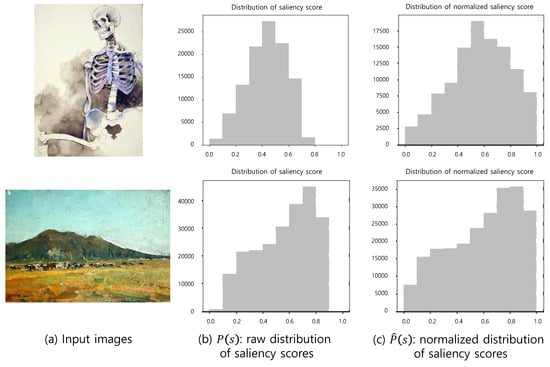
Figure 6. The normalized distributions of saliency scores for input images.

3.2. Building the Distribution of Saliency Scores of gtPatches

We aim to sample a patch that contains media stroke texture through the distribution of the saliency scores. For this purpose, we hire mechanical turks to mark the regions of an image that contains the media stroke texture. The saliency scores of these gtPatches that contain the regions form a distribution of saliency scores of gtPatch, which guides the expectation of gtPatch for an artwork image.

3.2.1. Capturing gtPatches from Mechanical Turks

To capture gtPatches, we hire ten mechanical turks. Before hiring mechanical turks, we execute a null test to exclude those turks who cannot do their job properly. We prepare several groundtruth images where the stroke media texture is very salient, and ask the turks to capture gtPatches on the images. According to the result, we exclude those turks who fails to satisfy our standard. We restrict the number of regions they mark as the same number of gtPatches and exclude the turks who fails to score 80% of correct answers. From this strategy, we tested 21 candidates to hire 10 turks for our study.

The hired turks are instructed to classify 100 artwork images according to artistic media. During the classification process, we instruct them to mark the regions in which they detect the media as illustrated in Figure 7. For correctly classified images, we samples $256\times 256$ sized patches that cover the regions as a gtPatch. Turks are instructed to mark at most three regions per images for the media stroke texture.

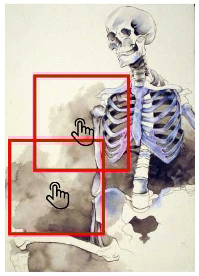
Figure 7. Example of gtPatch capturing. Regions selected by mechanical turks help recognize the artistic media of an artwork. Turks select at most three $256\times 256$-size of patches from a single artwork image.

We analyze the distribution of the saliency scores of the gtPatches sampled from an artwork image and determine the relationship between the saliency score and patches. Figure 8 illustrates an example. The saliency scores of the gtPatches are marked in the histogram of the saliency score distribution, and in this example, they are located between q1 and the median of the distribution.

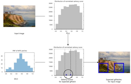
Figure 8. Estimating normalized distribution of saliency scores.

3.2.2. Building the Distribution of Saliency Scores of gtPatches

From one thousand images examined by mechanical turks, we capture 2316 gtPatches and estimate their saliency scores ($z_i$’s). From these scores, we build $Q\left(z\right)$, a distribution of saliency scores of gtPatches. This distribution gives us a guide to sample a gtPatch from an arbitrary artwork image.

3.3. Capturing Expected gtPatches from an Input Image

We sample five expected gtPatches per an artwork image. Our first candidate for an expected gtPatch is a patch whose saliency score is the mode of $Q\left(z\right)$ distribution. The next candidate patches are sampled by the next mode values in $Q\left(z\right)$. Since the distance between the neighboring patches is 10 pixels, the saliency scores of the neighboring pixels become very similar. Therefore, those patches that overlap the already chosen expected gtPatches in greater than 10% of their areas are ignored. In this process, we sample next expected gtPatches (See Figure 9).

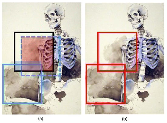
Figure 9. Excluding overlapped patches: (a) The black patch is a captured gtPatch. The dashed patch is a patch of next mode. But, it is excluded, since it is overlapped with the black gtPatch. The realline patch is captured next. (b) The two gtPatches.

However, a patch of identical saliency score may show very different stroke patterns, since the saliency score is the mean of the saliency values of the pixels in the patch. A patch that has a higher variance of the saliency values of the pixels is less adequate for a gtPatch than a patch that has lower variance (See Figure 10).

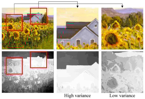
Figure 10. Examples of patches with identical saliency scores (0.67) but different variance values (0.16 and 0.33, respectively). The patch with high variance has a smaller probability of containing MTS than a patch with low variance.

4. Structure of Our Classifier

Our classifier is composed of several recognition modules, each of which is a pre-trained CNN [23]. The structure of our multi-column classifier is presented in Figure 11. The saliency scores of the patches on an input artwork image are estimated to sample patches, which are processed through a recognition module. To configure our recognition module, we examine several well-known CNN models for object recognition including AlexNet [33], VGGNet [34], GoogLeNet [35], ResNet [36], DenseNet [37], and EfficientNet [38]. To determine the CNN for the recognition module of our classifier and the number of modules of our classifier, we executed a baseline experiment to compare the accuracies on the various combinations on the CNN models and the number of modules on YMSet+.

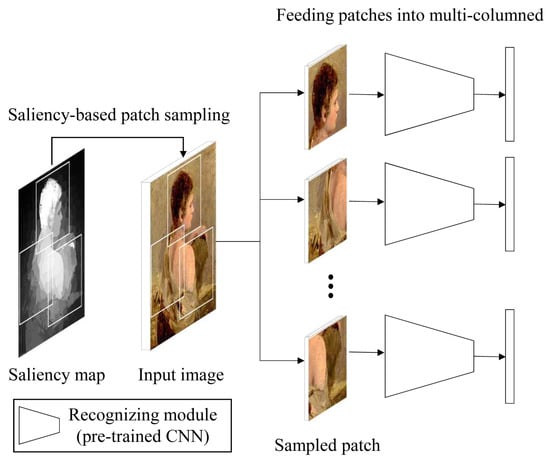
Figure 11. Our saliency-based multi-column classifier.

Our baseline experiment, is planed to find the best configuration by changing the recognition module and the number of modules. Since our model is a multi-columned structure consisted of several independent recognition modules, we test six most widely-used object recognizing CNN models including AlexNet [33], VGGNet [34], GoogLeNet [35], ResNet [36], DenseNet [37], and EfficientNet [38]. We also change the number of modules as 1, 3, and 5. We execute this experiment on YMSet+, which is composed of 6K contemporary artwork images of four media. The measured the accurcies of the eighteen combinations and illustrated them in Figure 12, where Figure 12a compares the number of modules per CNN models and Figure 12b compares CNN models. As a result of this experiment, we decide the best configuration of our model. A model of five modules of EfficientNet shows best accuracy.

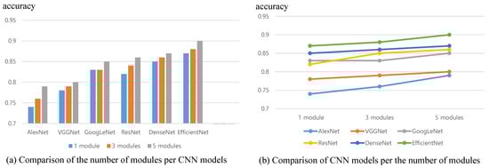
Figure 12. Result of our baseline experiment: Comparison of the CNN models and the number of modules.

5. Experiment

5.1. Data Collection

Because stroke texture plays a key role in recognizing artistic media in artwork images, we carefully collect artwork images that properly preserve media stroke texture. We employ YMSet [39], which is composed of the four most frequently used artistic media including pencil, oilpaint, watercolor and pastel. YMSet consists of 4 K contemporary artwork images in which media stroke texture is preserved. We extend YMSet to build YMSet+ which contains 6K artwork images. To train and to test our model, we separate YMSet into three parts: train set (70%), validation set (15%) and test set (15%).

To demonstrate that our model is effective for historical artwork images, we also construct artwork datasets from WikiArt, one of the largest artwork image collections on the internet. We build Wiki4, which is composed of 4K artwork images with the four most frequently used artistic media, and Wiki10, which is composed of 6K images with ten most frequently used media. The frequency of media in WikiArt is suggested in Figure 13, and the images in three datasets are illustrated in Figure 14.

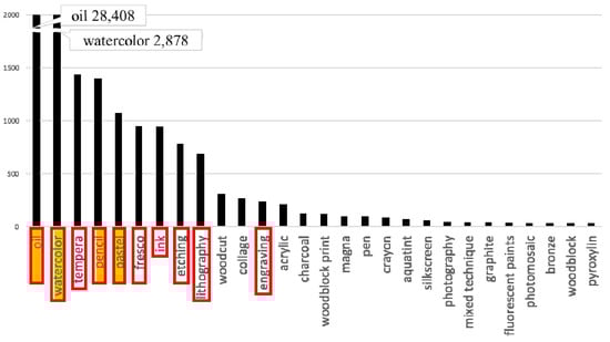
Figure 13. Frequency of the most frequently used media type from WikiArt: Yellow box denotes the media contained in YMSet+ and Wiki4, and red rectangle denotes those in Wiki10.

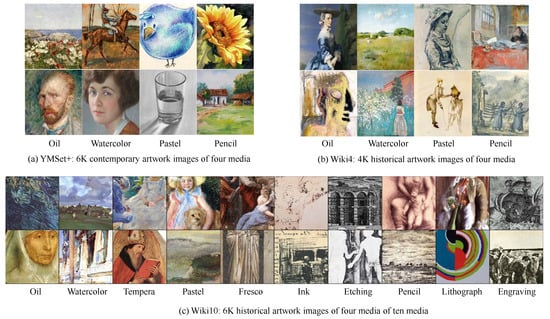
Figure 14. The collected datasets.

Since our model employs soft max operation to determine the most prominent media, the last layer of our model depends on the number of media to recognize. Therefore, in processing YMSet+ and Wiki4, the last layer of our model has four nodes, and Wiki10 dataset, the last layer is slightly modified to have ten nodes.

5.2. Experimental Setup

Our model is a multi-column structure of individual modules for recognizing artistic media. For the recognition module, we employ EfficientNet, which has the best performance in recognizing both objects and artistic media among CNN structures, discussed in Section 5. We employ Adam optimization as the optimization method, and we assign 0.0001 for the learning rate, 0.5 for weight decay and 40 for batch size. The learning rate is decreased by a factor of 10 whenever the error in the validation set stopped decreasing.

After training process using training dataset, we execute further hyper-parameter tuning on validation (development) dataset. Those parameters optimized on the validation dataset are employed for the test dataset to record the result of our model. The hyper-parameters include the number of units for layers, drop-out ratio, and learning rate.

The training was performed on an NVIDIA Tesla p40 GPU and took approximately two hours, depending on the size of the dataset. The performance is measured using the F1 score, which is the harmonic mean of precision and recall.

5.3. Training

We set the number of epoch as 100 for every training. We apply an early stop policy for the training, if our train process reaches a stable performance before 100 epochs. Figure 15 shows the decrease of the error during training of our model. Each curve means the error for train and validation(development).

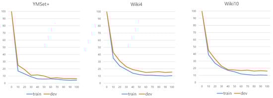
Figure 15. Decrease of error for the training process.

Our model trains individual recognizing networks including AlexNet, VGGNet, GoogLeNet, ResNet, DenseNet and EfficientNet with our datasets. The train times per epoch required for each model with our datasets are listed in Table 1. Since our study compares patch sampling strategies on an identical multi-columned structure, the training time in Table 1 is same for the three sampling strategies. We note that GoogLeNet requires exceptionally long training time.

Table 1. Time required for training a network for one epoch.

Module	Time per Epoch (min)
	YMSet+	Wiki4	Wiki10
AlexNet	$6.4$	$4.5$	$6.3$
VGGNet	$6.7$	$4.7$	$6.9$
GoogLeNet	$13.1$	$9.2$	$13.8$
ResNet	$7.3$	$4.8$	$7.1$
DenseNet	$7.6$	$5.1$	$7.5$
EfficientNet	$7.2$	$4.9$	$7.3$

5.4. Experiments

We execute three experiments in this study. The first experiment, which is a baseline experiment, is to find the best configuration of the multi-columned media recognition model. The second experiment is a measure on three patch sampling strategies to prove two arguments: (i) our strategy shows best performance and (ii) three sampling strategies show a consistent recognition patterns. The first argument is important, since the most important contribution of this study depends on it. The second argument is also important, since our sampling strategy inherits the recognition pattern of a multi-columned media recognition model. Since three comparing sampling strategies share an identical model, the characteristic of the model should be consistent on the sampling strategies. These two arguments are specified as research questions ($RQ$s) in Section 6. The third experiment is a measure on the recent deep learning-based methods to prove that our model shows best performance.

5.4.1. Experiment 1. Baseline Experiment

Our first experiment, a baseline experiment, is planed to find the best configuration by changing the recognition module and the number of modules. As explained in Section 4, we decide the best configuration of our model as five recognition modules of EfficientNet.

5.4.2. Experiment 2: Comparison on Patch Sampling Schemes

In our second experiment, we apply three datasets including YMSet+, Wiki4, and Wiki10 to the multi-columned media recognition model by alternating three sampling strategies. The first strategy is an object-based sampling [22], which samples the prominent regions from a portrait. The second one is a random sampling [23], which samples patches in a random way. The third one, our strategy, samples patches based on the criteria designed by estimating saliency and mimicking human strategy. An example of the sampled patches of these three strategies are illustrated in Figure 16. In this experiment, we measure F1 score, whose comparison is illustrated in Figure 17.

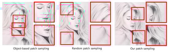
Figure 16. Comparison of three sampling schemes.

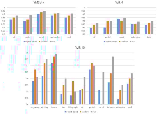
Figure 17. Comparison of F1 scores for three sampling schemes on three datasets: YMSet+, Wiki4 and Wiki10.

5.4.3. Experiment 3: Comparison on Recent Deep Learning-Based Recognition Methods

In our three experiment, we compare ours with three recent deep learning-based recognition methods. Lu et al. [20] proposed a postprocessing scheme for media recognition, while Sun et al. [14] employed a Gram matrix for media classification. We select these two methods for our comparison. Furthremore, we replace the VGGNet employed in Sun et al.’s work with cutting edge EfficientNet to improve their performance. Therefore three methods including Lu et al.’s work, Sun et al’s work and Sun et al’s work with EfficientNet are compared with ours. In this experiment, we measure F1 score, whose comparison is illustrated in Figure 18. This result shows that our model shows better performance than the existing deep learning-based methods.

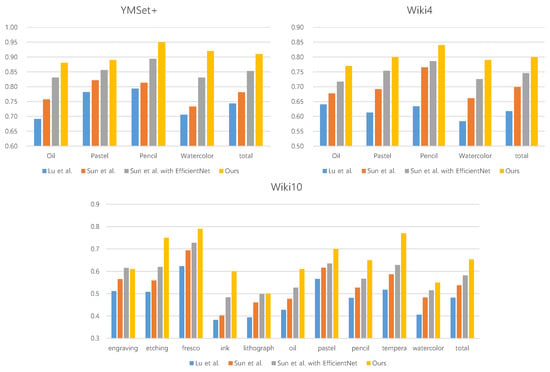
Figure 18. Comparison of F1 scores for three deep learning-based methods on three datasets: YMSet+, Wiki4 and Wiki10.

6. Analysis

The purpose of our analysis is to answer the following two research questions (RQs):

• (RQ1) Our sampling strategy shows best accuracies on confusion matrices.
• (RQ2) Our sampling strategy shows a significant different accuracies than the other sampling strategies.
• (RQ3) Why pastel shows worst accuracies for four media recognition through three approaches.
• (RQ4) Three sampling strategies show consistent recognition and confusion patterns.

6.1. Analysis1: Analysis of the Performance Compared to the Sampling Strategies

$RQ1$ is resolved by estimating the performances of the three strategies and comparing them. In Figure 17, we estimate accuracy, precision, recall and F1 score for the three different datasets. The performances of the individual medium as well as the total performances are compared. As illustrated in Figure 17, other strategies show better performance than ours in some specific media from some specific dataset. For example, other strategies show better performance than ours in watercolor from YMSet+. However, for the total performance, our strategy outperforms the other strategies in all measures and in all datasets. Therefore, we can resolve $RQ1$ that our sampling strategy shows better results than the other sampling strategies.

6.2. Analysis2: Analysis of Statistically Significant Difference of the Accuracies

$RQ2$ is resolved by t-test and Cohen’s d test on the F1-scores for Wiki10 media. Instead of YMSet+ and Wiki4 datasets whose dataset size is four, we choose Wiki10 dataset that has ten media. We configure five pairs for the comparison: (i) object-based sampling approach and ours, (ii) random sampling approach and ours, (iii) Lu et al. [20]’s method and ours, (iv) Sun et al. [14] and ours, (v) Sun et al. [14] with EfficientNet and ours.

For t-test, we build a hypothesis $H_0$ that there is no significant difference between ours and the opponent method. In case that p value is smaller than 0.05, then $H_0$ is rejected, which means that there is significant difference between two groups.

In computing Cohen’s d value, we notice that N, the number of sample, is 10, which is smaller than 50. Therefore, we estimate a corrected d value whose formula is:

$$d=\frac{M_E-M_C}{S{D}_{pooled}}\times \left(\frac{N-3}{N-2.25}\right)\times \sqrt{\frac{N-2}{N}}$$

The results of Analysis2 are presented in Table 2.

Table 2. p value for t-test and Cohen’s d value.

	t-Test		Cohen’s d
	p Value	${\mathit{H}}_0$	Corrected d Value	Effect Size
(i) object-based & ours	$0.03535$	reject	$0.82129$	large
(ii) random & ours	$0.34326$	not reject	$0.43590$	medium
(iii) Lu et al. [20] & ours	$0.00011$	reject	$1.12530$	large
(iv) Sun et al. [14] & ours	$0.00513$	reject	$0.87636$	large
(v) Sun et al. with EfficientNet & ours	$0.048644$	reject	$0.76138$	medium

From this analysis, we conclude that our approach produces significantly different results from object-based, Lu et al.’s, Sun et al.’s and Sun et al.’s with EfficientNet, but cannot produce significantly different result from random sampling approach. We also produce results with large effect size for object-based, Lu et al.’s and Sun et al.’s and medium effect size for random and Sun et al.’s with EfficientNet.

6.3. Analysis3: Analysis on the Poor Accuracy of Pastel

$RQ3$ is resolved by analyzing why pastel shows poor accuracy. It is interesting to analyze why pastel is the worstly recognized media for YMSet+ and Wiki4 through three approaches. The reason of the poor recognition of pastel is that pastel is mis-recognized as oilpainting. According to the confusion matrices in Figure 19, oil is the most confusing media for pastel through our three datasets and three approaches. However, pastel is not the most confusing media to oil.

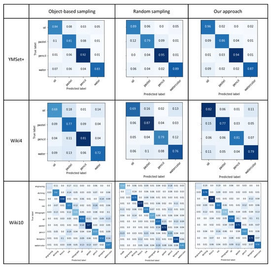
Figure 19. Comparison of confusion matrices: Row denotes the dataset and column denotes sampling strategies.

We analyze this difference comes from the point that oilpastel, which is a kind of a pastel, is labeled as pastel. However, the stroke patterns of oilpastel look very similar to those of oilpainting (See Figure 20). Therefore, all three approaches produces a confusing result in deciding oilpastel artwork images. They mis-classify those oilpastel artworks as oil instead of pastel.

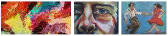
Figure 20. Oilpastel artworks similar to oilpainting artworks.

6.4. Analysis4: Analysis on the Consistency of the Sampling Strategies

It is important to show that the sampling strategies show a consistant recognition and confusion patterns for the media recognition process, which is addressed in $RQ4$. This analysis is executed in two aspects: proving the consistency for recognition pattern and for confusion pattern. We employ the confusion matrices from three datasets illustrated in Figure 19.

6.4.1. Analysis on the Consistency for Confusion Pattern

We define a confusion matric between two media for our analysis. Confusion metric between two media $m_i$ and $m_j$, which is denoted as $m_{ij}$, is defined as the sum of the elements in a confusion matrix $M_{ij}$ and $M_{ji}$. Note that $M_{ij}$ means that medium $m_i$ is misclassified into $m_j$, and $M_{ji}$ is vice versa. Therefore, a confusion metric $m_{ij}$ measures the magnitude of confusion in recognizing media $m_i$ and $m_j$.

To analyze the consistency of the sampling strategies, we categorize the confusion metric between two media into four groups based on the average $\mu$ and standard deviation $\sigma$ of the confusion metrics:

• strong distinguishing: $m_{ij}\le \mu -\sigma$
• weak distinguishing: $\mu -\sigma <m_{ij}\le \mu$
• weak confusing: $\mu <m_{ij}\le \mu +\sigma$
• strong confusing: $\mu +\sigma \le m_{ij}$

From the confusion type, we estimate matching type for three datasets. We define the matching type in four classes:

• strong match: $m_{ij}$’s from three datasets belong to the same confusion type.
• weak match: $m_{ij}$’s from three datasets belong to the same side of confusing or distinguishing, but they can be either strong or weak.
• weak mismatch: $m_{ij}$’s from three datasets belong to the opposite sides, but they are all weak distinguishing or confusing.
• strong mismatch: $m_{ij}$’s from three datasets do not belong to the one of three above cases.

In Figure 21, we present the confusion metric for each media pair from three datasets as well as their matching type. The summary of the matching type is suggested in Figure 22, where $100\%$ of the media pair from YMSet+ match, $66.7\%$ from Wiki4 and $82.3\%$ from Wiki10 match.

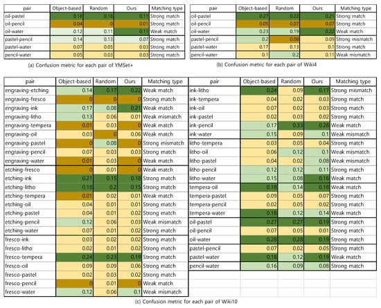
Figure 21. Confusion metrics and their matching types for each media pair from the three datasets and three sampling schemes.

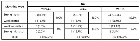
Figure 22. The matching results of confusion metric.

6.4.2. Analysis on the Consistency for Recognition Pattern

The diagonal element of a confusion matrix $M_{ii}$ plays a key role for the analysis on the consistency of the recognition pattern. $M_{ii}$ denotes the percentage of recognizing i medium into i medium. We define a recognition metric for i-th medium as $M_i$ ( we abbreviate double i’s as a single i).

Similar to the analysis on the confusion pattern, we categorize the recognition metric into four categories:

• strong unrecognizing: $M_i\le \mu -\sigma$
• weak unrecognizing: $\mu -\sigma <M_i\le \mu$
• weak recognizing: $\mu <M_i\le \mu +\sigma$
• strong recognizing: $\mu +\sigma \le M_i$

In Figure 23, we present the recognition metric for each medium from three datasets as well as their matching type. The summary of the matching type is suggested in Figure 24, where $100\%$ of the media pair from YMSet+ match, $50\%$ from Wiki4 and $80\%$ from Wiki10 match.

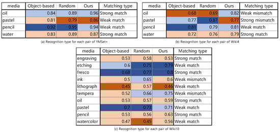
Figure 23. Recognition metrics and their matching types for each medium from the three datasets and three sampling schemes.

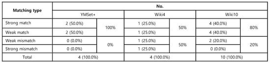
Figure 24. The matching results of recognition metric.

7. Conclusions and Future Work

In this paper, proposed a saliency-based sampling strategy that identifies patches containing stroke patterns of artistic media. To determine the relationship between saliency and media stroke pattern, we hired mechanical turks to mark gtPatches in artwork images and statistically analyzed the saliency scores of the patches. Based on the statistical relationship, we developed a strategy that samples patches with median saliency score and low variation of saliency values. We compared the performance of the existing patch sampling strategies and demonstrated that our saliency-based patch sampling strategy shows superior performance. Our strategy also shows a consistent recognition and confusion pattern with the existing strategies.

In future work, we plan to increase the level of details for recognizing target media. For example, artists can use only pastels to perform a variety of artistic techniques, such as smearing, scumbling and impasto, etc. These techniques are important for the deep understanding of artworks. We also plan to extend our study to be used as conditions of a generative model such as GAN to produce visually convincing artistic effects.

References

- Liu, G.; Yan, Y.; Ricci, E.; Yang, Y.; Han, Y.; Winkler, S.; Sebe, N. Inferring painting style with multi-task dictionary learning. In Proceedings of the International Conference on Artificial Intelligence 2015, Buenos Aires, Argentina, 25–31 July 2015; pp. 2162–2168. [Google Scholar]
- Florea, C.; Toca, C.; Gieseke, F. Artistic movement recognition by boosted fusion of color structure and topographic description. In Proceedings of the 2017 IEEE Winter Conference on Applications of Computer Vision (WACV), Santa Rosa, CA, USA, 24–31 March 2017; pp. 569–577. [Google Scholar]
- Liao, Z.; Gao, L.; Zhou, T.; Fan, X.; Zhang, Y.; Wu, J. An Oil Painters Recognition Method Based on luster Multiple Kernel Learning Algorithm. IEEE Access 2019, 7, 26842–26854. [Google Scholar] [CrossRef]
- Karayev, S.; Trentacoste, M.; Han, H.; Agarwala, A.; Darrell, T.; Hertzmann, A.; Winnemoeller, H. Recognizing image style. In Proceedings of the British Machine Vision Conference 2014, Nottingham, UK, 1–5 September 2014; pp. 1–20. [Google Scholar]
- Bar, Y.; Levy, N.; Wolf, L. Classification of artistic styles using binarized features derived from a deep neural network. In Proceedings of the Workshop at the European Conference on Computer Vision 2014, Zurich, Switzerland, 6–7 September 2014; pp. 71–84. [Google Scholar]
- Zhong, S.; Huang, X.; Xiao, Z. Fine-art painting classification via two-channel dual path networks. Int. J. Mach. Learn. Cybern. 2020, 11, 137–152. [Google Scholar] [CrossRef]
- Cetinic, E.; Lipic, T.; Grgic, S. Fine-tuning convolutional neural networks for fine art classification. Expert Syst. Appl. 2018, 114, 107–118. [Google Scholar] [CrossRef]
- van Noord, N.; Hendriks, E.; Postma, E. Toward Discovery of the Artist’s Style: Learning to recognize artists by their artworks. IEEE Signal Process. Mag. 2015, 32, 46–54. [Google Scholar] [CrossRef]
- Tan, W.; Chan, C.; Aguirre, H.; Tanaka, K. Ceci nést pas une pipe: A deep convolutional network for fine-art paintings classification. In Proceedings of the IEEE International Conference on Image Processing 2016, Phoenix, AZ, USA, 25–28 September 2016; pp. 3703–3707. [Google Scholar]
- Cetinic, E.; Grgic, S. Genre classification of paintings. In Proceedings of the International Symposium ELMAR 2016, Zadar, Croatia, 2–14 September 2016; pp. 201–204. [Google Scholar]
- Lecoutre, A.; Negrevergne, B.; Yger, F. Recognizing art styles automatically in painting with deep learning. In Proceedings of the Asian Conference on Machine Learning 2017, Seoul, Korea, 15–17 November 2017; pp. 327–342. [Google Scholar]
- Strezoski, G.; Worring, M. OmniArt: Multi-task deep learning for artistic data analysis. arXiv 2017, arXiv:1708.00684. [Google Scholar]
- Gatys, L.; Ecker, A.; Bethge, M. Image style transfer using convolutional neural networks. In Proceedings of the IEEE Conference on Computer Vision and Pattern Recognition 2016, Bhubaneswar, India, 27–28 July 2016; pp. 2414–2423. [Google Scholar]
- Sun, T.; Wang, Y.; Yang, J.; Hu, X. Convolution neural networks with two pathways for image style recognition. IEEE Trans. Image Process. 2017, 26, 4102–4113. [Google Scholar] [CrossRef] [PubMed]
- Chu, W.-T.; Wu, Y.-L. Deep correlation features for image style classification. In Proceedings of the 24th ACM International Conference on Multimedia, Amsterdam, The Netherlands, 15–19 October 2016; pp. 402–406. [Google Scholar]
- Chu, W.-T.; Wu, Y.-L. Image Style Classification based on Learnt Deep Correlation Features. IEEE Trans. Multimed. 2018, 20, 2491–2502. [Google Scholar] [CrossRef]
- Chen, L.; Yang, J. Recognizing the Style of Visual Arts via Adaptive Cross-layer Correlation. In Proceedings of the 27th ACM International Conference on Multimedia, Nice, France, 21–25 October 2019; pp. 2459–2467. [Google Scholar]
- Kong, S.; Shen, X.; Lin, Z.; Mech, R.; Fowlkes, C. Photo aesthetics ranking network with attributes and content adaptation. In Proceedings of the European Conference on Computer Vision 2016, Amsterdam, The Netherlands, 11–14 October 2016; pp. 662–679. [Google Scholar]
- Lu, X.; Lin, Z.; Jin, H.; Yang, J.; Wang, J.Z. RAPID: Rating pictorial aesthetics using deep learning. In Proceedings of the ACM International Conference on Multimedia 2014, Mountain View, CA, USA, 18–19 June 2014; pp. 457–466. [Google Scholar]
- Lu, X.; Lin, Z.; Shen, X.; Mech, R.; Wang, J.Z. Deep multi-patch aggregation network for image style, aesthetics, and quality estimation. In Proceedings of the IEEE International Conference on Computer Vision 2015, Santiago, Chile, 11–18 December 2015; pp. 990–998. [Google Scholar]
- Mai, L.; Jin, H.; Liu, F. Composition-preserving deep photo aesthetics assessment. In Proceedings of the IEEE Conference on Computer Vision and Pattern Recognition 2016, Las Vegas, NV, USA, 27–30 June 2016; pp. 497–506. [Google Scholar]
- Anwer, R.; Khan, F.; Weijer, J.V.; Laaksonen, J. Combining holistic and part-based deep representations for computational painting categorization. In Proceedings of the 2016 ACM on International Conference on Multimedia Retrieval, New York, NY, USA, 6–9 June 2016; pp. 339–342. [Google Scholar]
- Yang, H.; Min, K. A Multi-Column Deep Framework for Recognizing Artistic Media. Electronics 2019, 8, 1277. [Google Scholar] [CrossRef]
- Sandoval, C.; Pirogova, E.; Lech, M. Two-Stage Deep Learning Approach to the Classification of Fine-Art Paintings. IEEE Access 2019, 7, 41770–41781. [Google Scholar] [CrossRef]
- Bianco, S.; Mazzini, D.; Napoletano, P.; Schettini, R. Multitask Painting Categorization by Deep Multibranch Neural Network. Expert Syst. Appl. 2019, 135, 90–101. [Google Scholar] [CrossRef]
- Mensink, T.; van Gemert, J. The Rijksmuseum Challenge: Museum-centered visual recognition. In Proceedings of the ACM International Conference on Multimedia Retrieval 2014, Glasgow, UK, 1–4 April 2014; p. 451. [Google Scholar]
- Mao, H.; Cheung, M.; She, J. DeepArt: Learning joint representations of visual arts. In Proceedings of the ACM International Conference on Multimedia 2017, Mountain View, CA, USA, 23–27 October 2017; pp. 1183–1191. [Google Scholar]
- Gupta, A.K.; Seal, A.; Prasad, M.; Khanna, P. Salient object detection techniques in computer vision—A survey. Entropy 2020, 20, 1174. [Google Scholar] [CrossRef] [PubMed]
- Cheng, M.-M.; Mitra, N.J.; Huang, X.; Torr, P.H.S.; Hu, S.-M. Global contrast based salient region detection. IEEE Trans. Pattern Anal. Mach. Intell. 2014, 37, 569–581. [Google Scholar] [CrossRef]
- Lu, S.; Mahadevan, V.; Vasconcelos, N. Learning optimal seeds for diffusion-based salient object detection. In Proceedings of the IEEE Conference on Computer Vision and Pattern Recognition 2014, Columbus, OH, USA, 23–28 June 2014; pp. 2790–2797. [Google Scholar]
- Zhang, J.; Sclaroff, S.; Lin, Z.; Shen, X.; Price, B.; Mech, R. Minimum barrier salient object detection at 80 fps. In Proceedings of the IEEE International Conference on Computer Vision 2015, Santiago, Chile, 7–13 December 2015; pp. 1404–1412. [Google Scholar]
- Zhu, W.; Liang, S.; Wei, Y.; Sun, J. Saliency optimization from robust background detection. In Proceedings of the IEEE Conference on Computer Vision and Pattern Recognition (CVPR), Columbus, OH, USA, 23–28 June 2014; pp. 2814–2821. [Google Scholar]
- Krizhevsky, A.; Sutskever, I.; Hinton, G.E. Imagenet classification with deep convolutional neural networks. In Proceedings of the Advances in Neural Information Processing Systems 2012, Lake Tahoe, NV, USA, 3–6 December 2012; pp. 1097–1105. [Google Scholar]
- Simonyan, K.; Andrew, Z. Very deep convolutional networks for large-scale image recognition. arXiv 2014, arXiv:1409.1556. [Google Scholar]
- Szegedy, C.; Liu, W.; Jia, Y.; Sermanet, P.; Reed, S.; Anguelov, D.; Erhan, D.; Vanhoucke, V.; Rabinovich, A. Going deeper with convolutions. In Proceedings of the IEEE Conference on Computer Vision and Pattern Recognition 2015, Boston, MA, USA, 7–12 June 2015; pp. 1–9. [Google Scholar]
- He, K.; Zhang, X.; Ren, S.; Sun, J. Deep residual learning for image recognition. In Proceedings of the IEEE Conference on Computer Vision and Pattern Recognition 2016, Las Vegas, NV, USA, 27–30 June 2016; pp. 770–778. [Google Scholar]
- Huang, G.; Liu, Z.; Maaten, L.V.D.; Weinberger, K.Q. Densely connected convolutional networks. In Proceedings of the IEEE Conference on Computer Vision and Pattern Recognition 2017, Honolulu, HI, USA, 21–26 July 2017; pp. 4700–4708. [Google Scholar]
- Tan, M.; Le, Q. EfficientNet: Rethinking Model Scaling for Convolutional Neural Networks. In Proceedings of the International Conference on Machine Learning 2019, Long Beach, CA, USA, 9–15 June1 2019; pp. 6105–6114. [Google Scholar]
- Yang, H.; Min, K. A Deep Approach for Classifying Artistic Media from Artworks. KSII Trans. Internet Inf. Syst. 2019, 13, 2558–2573. [Google Scholar]
Publisher’s Note: MDPI stays neutral with regard to jurisdictional claims in published maps and institutional affiliations. |
© 2021 by the authors. Licensee MDPI, Basel, Switzerland. This article is an open access article distributed under the terms and conditions of the Creative Commons Attribution (CC BY) license (https://creativecommons.org/licenses/by/4.0/).