Empirical Analysis of Rank Aggregation-Based Multi-Filter Feature Selection Methods in Software Defect Prediction

Abstract

Selecting the most suitable filter method that will produce a subset of features with the best performance remains an open problem that is known as filter rank selection problem. A viable solution to this problem is to independently apply a mixture of filter methods and evaluate the results. This study proposes novel rank aggregation-based multi-filter feature selection (FS) methods to address high dimensionality and filter rank selection problem in software defect prediction (SDP). The proposed methods combine rank lists generated by individual filter methods using rank aggregation mechanisms into a single aggregated rank list. The proposed methods aim to resolve the filter selection problem by using multiple filter methods of diverse computational characteristics to produce a dis-joint and complete feature rank list superior to individual filter rank methods. The effectiveness of the proposed method was evaluated with Decision Tree (DT) and Naïve Bayes (NB) models on defect datasets from NASA repository. From the experimental results, the proposed methods had a superior impact (positive) on prediction performances of NB and DT models than other experimented FS methods. This makes the combination of filter rank methods a viable solution to filter rank selection problem and enhancement of prediction models in SDP.

1. Introduction

Software development lifecycle (SDLC) is a defined process specifically created for the development of reliable and high-quality software systems. The stages embedded in SDLC such as requirement gathering, requirement analysis, system design, system development and maintenance are stepwise and must be strictly observed to ensure a timely and efficient software system [1,2,3]. Nonetheless, human errors or mistakes are inevitable even though most of the stages in SDLC are conducted by professionals. In recent times, these errors tend to be more profound as modern software systems are intrinsically large, with co-dependent components and modules. Consequently, these errors if not fixed immediately will bring about defective software systems and ultimately software failure. In other words, having defects in software systems will lead to degraded and unreliable software systems. In addition, software failures can generate dissatisfaction from end-users and stakeholders alike as failed software does not meet user requirement(s) after resources (time and effort) have been expiated [4,5]. Hence, it is imperative to consider early prediction and detection of software defects before software release. Early detection of defective modules or components in a software system will grant spontaneous rectification of such modules or components and judicious usage of available resources [6,7].

Software defect prediction (SDP) is the adoption of machine learning (ML) techniques for determining the defectiveness of software modules or components. Specifically, SDP is the application of ML techniques on software defect datasets which are characterized by software metrics (as features) to ascertain defects in software modules or components [8,9,10]. From studies, both supervised and unsupervised types of ML techniques have been proposed and implemented for SDP [11,12,13,14,15,16]. However, the prediction performance of SDP models categorically depends on the nature (quality) and characteristics of software datasets used in developing SDP models. Software metrics used in characterizing the reliability and quality of software systems is directly proportional to the size of software systems. That is, large and robust software systems will require many software metric mechanisms to generate features that best describes the quality of such software systems [17,18]. Invariably, software systems with a high number of features as a result of the proliferation of software metrics often consist of redundant and noisy features. This phenomenon is usually referred to as a high dimensionality problem. Studies have shown that high dimensionality problem negatively affects the prediction performances of SDP models [19,20,21]. It is established in the literature that feature selection (FS) method is a prominent way to solve high dimensionality problem. Mainly, all FS methods cull only irredundant and important software features from the original software defect dataset for any SDP processes [22,23,24].

The application of FS method will result in the creation of a subset of the initial dataset. This subset contains the selection of important and irredundant features from a set of irrelevant and excessive features, thereby resolving high dimensionality of a given dataset. That is, FS methods capture only the important features while making sure the quality of the dataset is intact. This ultimately resolves the high dimensionality problem in software defect datasets. FS is an important data pre-processing task as it improves the quality of dataset (i.e., noise removal), reduces computational complexity and mostly improves the prediction performances of prediction models [25,26]. In general, FS methods can be divided into groups: filter feature selection (FFS) and wrapper feature selection (WFS). FFS methods assess and rank features of a dataset based on mathematical or statistical measures. Thereafter, top-ranked features are selected based on a pre-determined threshold value [22,23]. FFS are simple and are independent of ML classification algorithms (often referred to as baseline classifiers). Unlike FSS, WFS method assesses and select features based on its positive influence toward improving the accuracy of the underlying baseline classifier. This makes WFS computationally expensive and hard to implement [27,28,29]. Based on these discriminatory qualities, researchers often choose and implement FSS methods in SDP [19,30]. However, it was observed that some studies have investigated the effect of FSS methods on prediction performances of SDP models with conflicting research outcomes [16,20,23,24]. These conflicting research findings can be attributed to the selection of an appropriate FFS method and the issue of incomplete and disjoint feature ranking of FFS methods in SDP. Specifically, with the variety of different FFS methods, selecting the most appropriate FFS method that will give the best performance is a difficult task [19,31]. This is as a result of FFS methods having diverse and distinct underlining computational characteristics in their respective approaches, hence, making the selection of the FFS method in SDP is a hard choice. This study proposes as a solution, rank-aggregation based multi-filter feature selection methods for SDP. The proposed methods aim to address the filter selection problem by aggregating rank lists from multiple filter FS methods of diverse computational characteristics to produce a more stable (i.e., non-disjoint) and complete feature rank list better than individual filter methods employed.

The main contributions of this study are as follows:

• Development of novel rank-aggregation based multi-filter feature selection methods.
• Empirical evaluation and analysis of the performance of rank-aggregation based multi-filter feature selection methods in SDP.

2. Related Works

High dimensionality has been regarded as a data quality problem that dampens the prediction efficacies of models in SDP. That is, the presence of irrelevant and redundant software features as a result of the proliferation of software features (metrics) used to characterize the reliability and quality of a software harms the effectiveness of SDP models. From existing studies, FS methods are used to tackle high dimensionality problem by culling only important features. Hence, many studies have proposed and developed diverse FS methods for SDP.

Cynthia et al. [32] experimented on the effect of FS methods on SDP models using various evaluation metrics. They concluded that the selection of important features from a dataset can positively improve the prediction performance of models while substantially reducing the training time and FFS had the best impact in their study. Nonetheless, their study had a limitation in the type of filter-based feature selection considered.

Balogun et al. [22] in their study, investigated the impact of FS methods on models in SDP based on applied search methods. The performances of eighteen FS methods using four classifiers were analyzed. Their findings also support the notion of using FS methods in SDP; however, the respective effect of FS methods on SDP varies across datasets and applied classifiers. Additionally, they posited that filter-based feature selection methods had stable accuracy values than other studied FS methods. Nonetheless, the filter methods selection problem still lingers as the performance of the filter-based FS methods depends on the dataset and classifier used for the SDP process.

In another study, Balogun et al. [23] conducted an extensive empirical study on the impact of FS methods on SDP models based on some contradictions and inconsistencies in existing studies as highlighted by Ghotra et al. [20] and Xu, et al. [24]. From their experimental results, they further established that the efficacy of FS methods depends on dataset and classifier deployed. Hence, there are no best FS methods. This further supports the filter selection problem methods as each filter-based FS methods works differently.

Jia [33] proposed a hybrid FS method based on combining the strength of 3 filter methods (chi-squared, information gain and correlation filter) for SDP. The average ranking of each feature was deduced from the respective rank list and the TopK features were selected. Their experimental results showed that models based on hybrid FS method were better than models from the individual filter methods. Nonetheless, the effectiveness of averaging rank lists of features can be affected by the skewed ranks of each feature [34]. Besides, selecting arbitrary TopK features may not be the best method as useful features may be omitted during the selection process [32].

Wang et al. [35] investigated the ensemble of FS methods in SDP to solve the filter selection problem. 17 ensemble methods were implemented using 18 different filter FS methods. The ensemble methods were based on averaging the ranks of features from individual rank lists. From their experimental results, they reported the superiority of the ensemble approaches. However, similar to Jia [33], averaging rank lists of features can be affected by the skewed ranks of each feature.

Xia et al. [36] hybridized ReliefF and correlation analysis for selection of features in metric-based SDP. the proposed method (ReliefF-Lc) checks correlation and redundancy between modules concurrently. From their experimental results, ReliefF-Lc outperforms other experimented methods (IG and REF). Additionally, Malik et al. [37] conducted an empirical comparative study on the use of an attribute rank method. In particular, the applicability of principal component analysis (PCA) with the ranker search method as a filter FS method was investigated. They concluded that applying PCA with ranker search method in the SDP process can improve the effectiveness of classifiers in SDP. Although their findings cannot be generalized due to the limited scope of their study, however, they coincide with existing SDP studies on the application of FS methods in SDP.

Iqbal and Aftab [30] developed an SDP framework using multi-filter FS and multi-layer perceptron (MLP). Besides, a random over-sampling (ROS) technique was integrated to address the inherent class imbalance problem. The proposed multi-filter was developed using correlation feature selection (CFS) with 4 different search methods. From their experimental results, they concluded that the multi-filter method with ROS outperforms other experimented methods.

Consequently, FS methods are efficient in minimizing or reducing features of a dataset and amplifying the efficiency of models in SDP. Notwithstanding, selecting an appropriate filter-based FS method is an open problem. Hence, this study presents an empirical analysis of the impact of rank aggregation-based multi-filter FS method on prediction performances of SDP models.

3. Methodology

In this section, the classification algorithms, filter-based FS methods, proposed rank aggregation-based multi-filter, experimental framework, software defect datasets and performance evaluation metrics are presented and discussed.

3.1. Classification Algorithms

Decision Tree (DT) and Naïve Bayes (NB) algorithms are used to fit base-line prediction models in this study. DT and NB algorithms have been widely implemented in numerous existing studies with satisfactory prediction capabilities. Besides, findings have shown that DT and NB work well with class imbalance [22,38]. Table 1 presents parameter settings of DT and NB algorithms as used in this study.

Table 1. Classification Algorithms.

Classification Algorithms	Parameter Settings
Decision Tree (DT)	ConfidenceFactor = 0.25; MinObj = 2
Naïve Bayes (NB)	NumDecimalPlaces = 2; NumAttrEval = Normal Dist.

3.2. Filter Feature Selection

3.2.1. Chi-Square (CS)

Chi-square (CS) filter method is a statistics-based FS method that tests the independence of a feature to the class label by generating a score to determine the level of independence. The higher the generated score, the higher the dependent relationship between a feature and the class label. CS can be mathematically represented as:

$$X^2\left(r, c_i\right)=\frac{N{\left[P\left(r, c_i\right)P\left(\overline{r}, {\overline{c}}_i\right)–P\left(r, {\overline{c}}_i\right)P\left(\overline{r}, c_i\right)\right]}^2}{\left[P\left(r\right)P\left(\overline{r}\right)P\left({\overline{c}}_i\right)P\left(c_i\right)\right]}$$

(1)

3.2.2. ReliefF (REF)

ReliefF (REF) filter method deploys sampling method on a given dataset and then locates the nearest neighbors from the same and alternate classes. The features of the sampled instances are compared with those of its neighborhood and then subsequently assign a relevant score of each feature. REF is an instance-based FS method that can be applied on noisy and incomplete datasets. It can ascertain dependencies amongst features with low bias.

3.2.3. Information Gain (IG)

Information Gain (IG) filter method selects relevant features by reducing the uncertainties attributed with identifying the class label based on the information theory mechanism when the value of the feature is unknown. The information theory assesses and culls top features before commencing the training process. The entropy of an instance (say X) can be defined as thus:

$$H\left(X\right)=-{\displaystyle \sum }_i{P}_{x_{i }}{\mathit{log}}_2{P}_{x_i}$$

(2)

where $P_{x_i}$ represents the prior probabilities of X.

The entropy of X given another instance Y is represents as:

$$H\left(X|Y\right)=–{\displaystyle \sum }_i{P}_{y_{j }}{\displaystyle \sum }_i{P}_{x_i|y_{j }}{\mathit{log}}_2{P}_{x_i|y_j}$$

(3)

Hence, the entropy is given as the level by which the entropy of X reduces to show additional information concerning X as given by Y, and is defined thus:

$$IG\left(X|Y\right)=H\left(X\right)–H(X|Y)$$

(4)

3.3. Rank Aggregation-Based Multi-Filter Feature Selection (RMFFS) Method

The proposed RMFFS is based on taking into consideration and combining the strengths of individual filter ranks methods. The essence of this is to resolve the filter method selection problem by considering multiple rank lists in the generation and subsequent selection of top-ranked features to be used in the prediction process. As depicted in Algorithm 1, the individual rank list from CS, REF, and IG filter methods are generated from the given dataset. These individual rank lists are mutually exclusive as each filter methods considered are based on different computational characteristics. This is to ensure diverse representations of features to be selected for the prediction process. Thereafter, the generated rank lists are aggregated together using rank aggregation functions as presented in Table 2. The respective rank aggregation function combines the individual rank lists into a single aggregated list by leveraging on the relevance score attributed to each feature on the individual rank lists. Minimum and maximum rank functions select the minimum and maximum relevance score, respectively, produced by the aggregated rank list. The range rank function selects features from the aggregated list based on the range value computed from the relevance scores. The arithmetic mean, geometric mean and harmonic mean rank functions combine the individual rank lists into a single aggregated list by computing the arithmetic mean, geometric mean and harmonic mean, respectively, on the relevance score attributed to each feature on the individual rank lists. This is to give equal representation and consideration to each feature from each rank list. Features on the aggregated list with high relevance scores indicates that such features are ranked low in the individual rank list and as such can be dropped. A novel dynamic and automatic threshold value based on geometric mean function are applied to the aggregated list to select relevant features. The geometric mean of the aggregated relevance score is computed and features with aggregated relevance score less than or equal to the computed threshold values are selected. Geometric mean functions consider the dependency amongst the features and the compounding effect in its computation. Finally, optimal features are selected as the resulting features of the RMFFS method.

Algorithm 1 Rank Aggregation based Multi-Filter Feature Selection (RMFFS) Method

Input: N—Number of Filter Rank Method = {CS, REF, IG} T—Threshold value for optimal features selections = ${\left({\displaystyle \prod }_{i=1}^n{X}_i\right)}^{\raisebox{1ex}{$1$}\!\left/ \!\raisebox{-1ex}{$n$}\right.}$ = $\sqrt[n]{X_1{X}_2{X}_{3 }\dots X_n}$ A—Aggregators A = {min{$R_1\left(a_{1\dots n}\right), R_2\left(a_{1\dots n}\right), \dots R_m\left(a_{1\dots n}\right)$}, max{$R_1\left(a_{1\dots n}\right), R_2\left(a_{1\dots n}\right), \dots R_m\left(a_{1\dots n}\right)$},   range{$R_1\left(a_{1\dots n}\right), R_2\left(a_{1\dots n}\right), \dots R_m\left(a_{1\dots n}\right)\},$mean{$\left({\displaystyle \sum }_{i=1}^m{R}_i\left(a_{1\dots n}\right)\right)\times \raisebox{1ex}{$1$}\!\left/ \!\raisebox{-1ex}{$m$}\right.$}, g.mean{${\displaystyle \prod }_1^m{R}_i{\left(a_{1\dots n}\right)}^{\raisebox{1ex}{$1$}\!\left/ \!\raisebox{-1ex}{$m$}\right.}$}, h.mean{$\raisebox{1ex}{$m$}\!\left/ \!\raisebox{-1ex}{${{\displaystyle \sum }}_{i=1}^m\raisebox{1ex}{$1$}\!\left/ \!\raisebox{-1ex}{$R_i\left(a_{1\dots n}\right)$}\right.$}\right.$} P—Aggregated Features Output: $P_t^{\prime }$—Optimal Features Selected From Aggregated Rank List based on T 1.  for $i=1$to N {do 2.    Generate Rank list Rn for each filter rank method i 3.              } 4. Generate Aggregated Rank list using Aggregator functions:   for i = 1 to $A_n\{ do$ 5.       $P_i=A_i$ 6.       for i = 1 to $P_i$ { 7.             if ($P_i\le$ T) 8.             $P^{\prime } =P_i$ //Select optimal features from $P^{\prime }$ based on T 9.            } 10.  $P_t^{\prime }$ = $P_{}^{\prime }$ 11.      return $P_t^{\prime }$ 12.           }

Table 2. Rank Aggregation Methods.

Aggregators	Formula	Description
Min ()	min{$R_1\left(a_{1\dots n}\right), R_2\left(a_{1\dots n}\right), \dots R_m\left(a_{1\dots n}\right)$}	Selects the minimum of the relevance scores produced by the aggregated rank list
Max ()	max{$R_1\left(a_{1\dots n}\right), R_2\left(a_{1\dots n}\right), \dots R_m\left(a_{1\dots n}\right)$}	Selects the maximum of the relevance scores produced by the aggregated rank list
Range ()	range{$R_1\left(a_{1\dots n}\right), R_2\left(a_{1\dots n}\right), \dots R_m\left(a_{1\dots n}\right)$}	Selects the range of the relevance scores produced by the aggregated rank list
Mean ()	mean{$\left({\displaystyle \sum }_{i=1}^m{R}_i\left(a_{1\dots n}\right)\right)\times \raisebox{1ex}{$1$}\!\left/ \!\raisebox{-1ex}{$m$}\right.$	Selects the mean of the relevance scores produced by the aggregated rank list
Geometric Mean ()	g.mean{${\displaystyle \prod }_1^m{R}_i{\left(a_{1\dots n}\right)}^{\raisebox{1ex}{$1$}\!\left/ \!\raisebox{-1ex}{$m$}\right.}$}	Selects the geometric mean of the relevance scores produced by the aggregated rank list
Harmonic Mean ()	h.mean{$\raisebox{1ex}{$m$}\!\left/ \!\raisebox{-1ex}{${{\displaystyle \sum }}_{i=1}^m\raisebox{1ex}{$1$}\!\left/ \!\raisebox{-1ex}{$R_i\left(a_{1\dots n}\right)$}\right.$}\right.$}	Selects the harmonic mean of the relevance scores produced by the aggregated rank list

3.4. Software Defect Datasets

Table 3 presents the software defect datasets used for training and testing SDP models in this study. These datasets are culled from NASA repository and have been widely used in SDP. Specifically, the cleaned version of NASA datasets was used in the experimentation [39,40]. Table 2 shows a description of the selected datasets with their respective number of features and number of instances.

Table 3. Description of selected NASA datasets.

Datasets	Number of Features	Number of Modules
CM1	38	327
KC1	22	1162
KC2	22	522
KC3	40	194
MW1	38	250
PC1	38	679
PC3	38	1077
PC4	38	1287
PC5	39	1711

3.5. Performance Evaluation Metrics

For evaluation of ensuing SDP models, Accuracy, F-Measure, and Area under Curve (AUC) were selected. These evaluation metrics have been widely used and proven to be reliable in SDP studies [7,41,42].

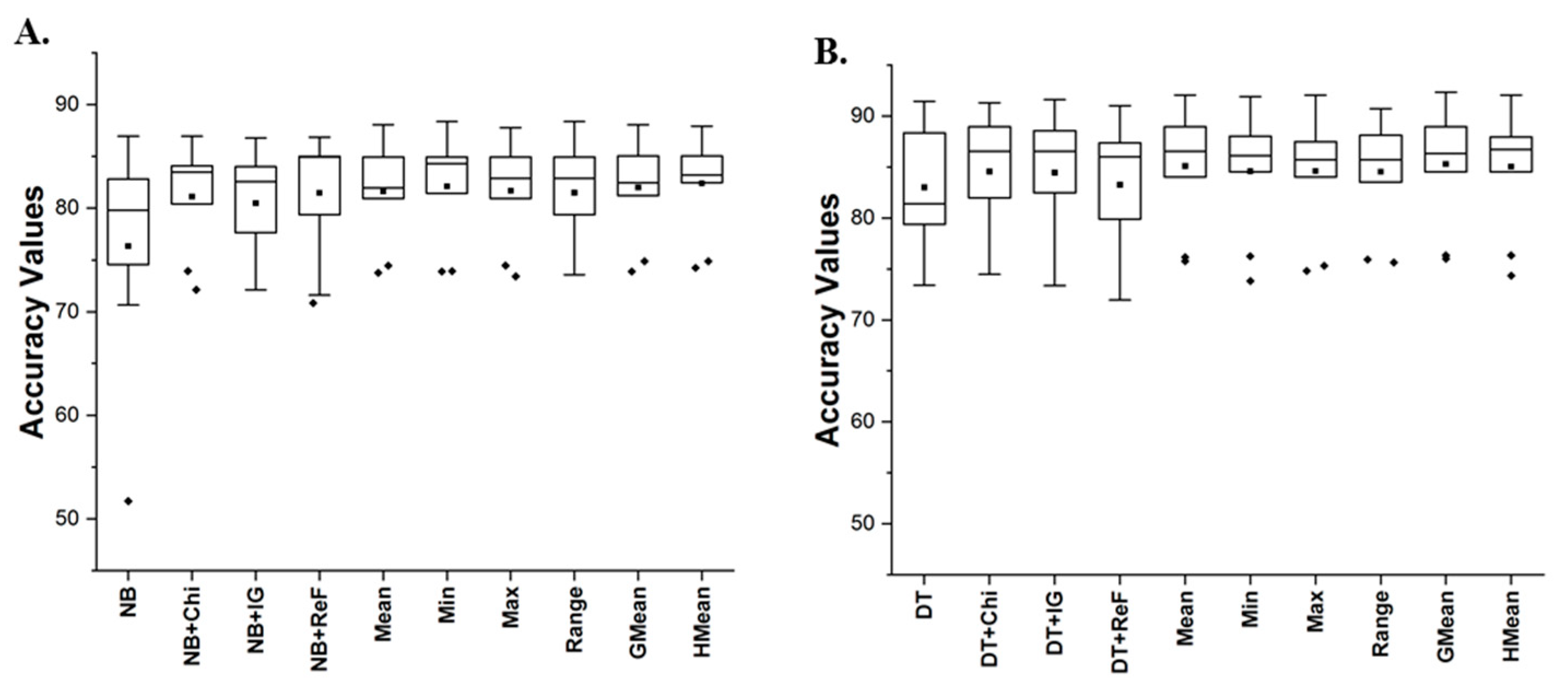
• Accuracy is the number or percentage of correctly predicted data out of all total amount of data.

  $$\mathrm{Accuracy}=\frac{TP+TN}{TP+FP+FN+TN}$$

  (5)
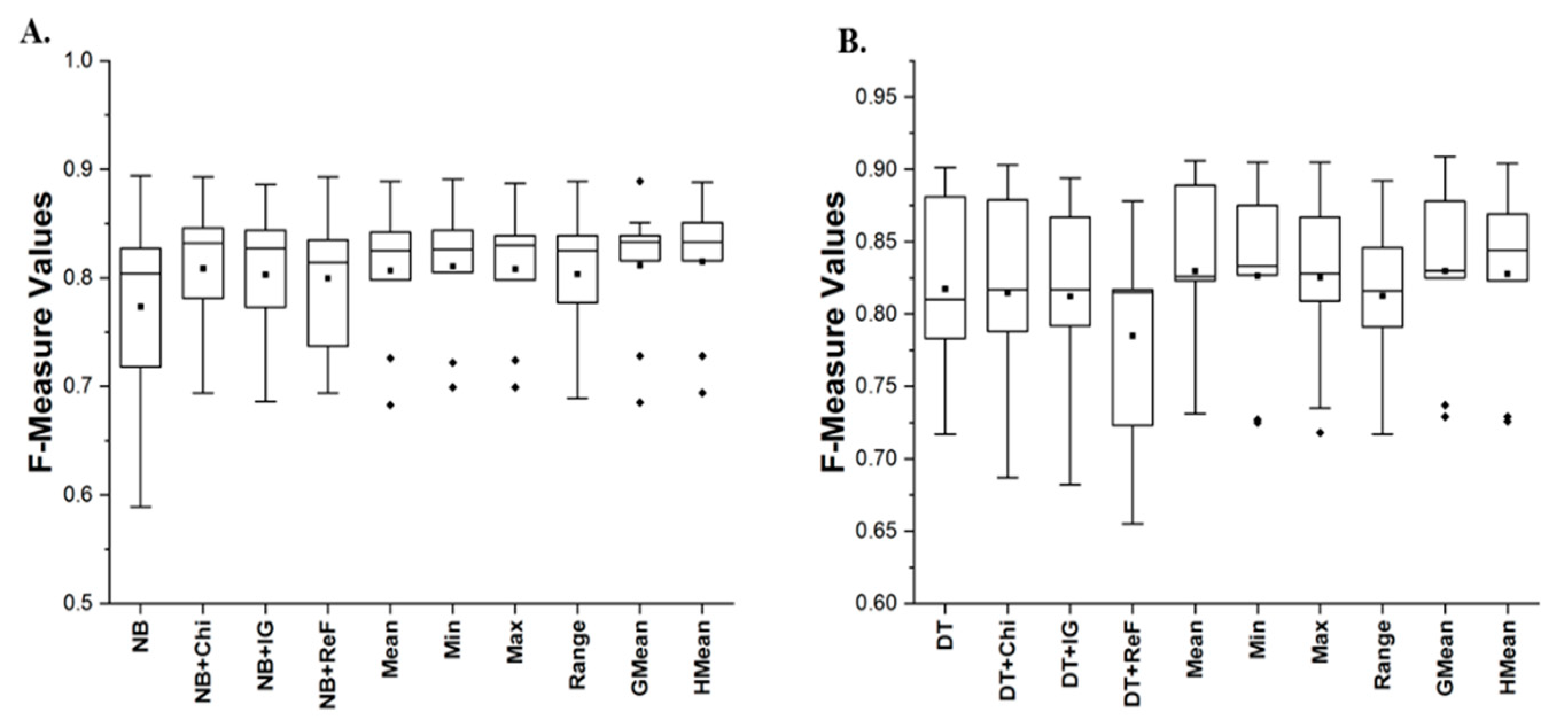
• F-Measure is defined as the weighted harmonic mean of the test’s precision and recall

  $$\mathrm{F}-\mathrm{Measure}=2\times \left(\raisebox{1ex}{$\mathrm{Precision}\times \mathrm{Recall}$}\!\left/ \!\raisebox{-1ex}{$\mathrm{Precision}+\mathrm{Recall}$}\right.\right)$$

  (6)
• The Area under Curve (AUC) indicates the trade-off between TP and FP. It shows an aggregate measure of performance across all possible classification thresholds.

$\mathrm{Recall}=\left(\frac{TP}{TP+FN}\right)$, $\mathrm{Precision}=\left(\frac{TP}{TP+FP}\right)$, TP = True Positive (implies the accurate classification); FP = False Positive (means inaccurate classification); TN = True Negative (implies accurate misclassification); FN = False Negative (implies inaccurate misclassification).

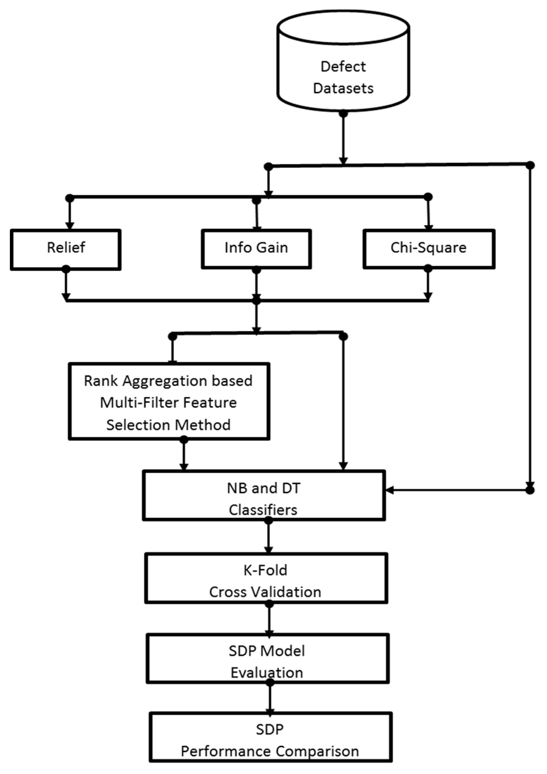
3.6. Experimental Framework

The experimental framework of this study as depicted in Figure 1 is presented and discussed in this section.

Figure 1. Experimental Framework.

To assess effects of proposed RMFFS methods on prediction performances of SDP models, software defect datasets (See Table 3) were used to build SDP models based on NB and DT classifiers (See Table 1). Different scenarios are experimented to have unbiased and standard performance comparison of the ensuing SDP models.

• Scenario 1 considered the application of the baseline classification algorithm (NB and DT) on the original defect datasets. In this case, NB and DT will be trained and tested with the original defect datasets. This is to determine the prediction performances of the baseline classifiers on the defect datasets.
• Scenario 2 is based on the application of each filter rank method (CS, REF, and IG) on the baseline classifiers. This is to determine and measure the individual effect of each filter rank methods on prediction performances of NB and DT over the selected defect datasets.
• Scenario 3 indicates the application of the proposed RMFFS method on the baseline classifiers. Just as in Scenario 2, this is to determine and measure the effectiveness of the proposed RMFFS method on prediction performances of NB and DT over the selected defect datasets.

Experimental results and findings based on the aforementioned scenarios will be used to answer the following research questions.

• RQ1. How effective are the proposed RMFFS methods compared to individual filter FS methods?
• RQ2. Which of RMFFS methods had the highest positive impact on the prediction performance of SDP models?

Ensuing SDP models from each scenario will be developed and evaluated based on 10-fold cross-validation (CV) technique. The application of 10-fold CV technique is to avoid data variability problems and to produce SDP models with low bias and variance [43,44,45,46]. Besides, CV techniques have been widely used in many existing studies with SDP being no exception. The prediction performances of ensuing models from each scenario will be measured using selected performance metrics (See Section 3.5) and their predictive performance will be analyzed and compared. All experiments are carried out using the WEKA machine learning tool [47].

4. Results and Discussion

In this section, experimental results based on the experimental framework as illustrated in Figure 1 is presented and discussed.

Figure 2, Figure 3 and Figure 4 presents box-plots representation of the prediction performances based on accuracy, AUC and f-measure of NB and DT models with No FS method, IG, REF, CS and proposed RMFFS methods. Figure 2 presents the accuracy values of NB and DT models with respective FS (IG, CS, REF and RMFFS) and No FS methods. Both NB and DT had good accuracy values on the software defect dataset. However, the application of individual FS methods (IG, CS and REF) further improves the accuracy values of NB and DT. This can be seen in their respective average accuracy values as depicted in Figure 2. Application of NB and DT models with No FS method recorded average accuracy values of 76.33 and 83.01%, respectively. However, CS averagely improved the accuracy values of NB (81.12%) and DT (84.56%) by +6.28 and +1.87%. A similar occurrence was observed on prediction models with REF (NB: 81.47% and DT: 83.26%) with improved average accuracy values of +6.73 and +0.3%, respectively. Additionally, IG averagely improved the accuracy values of NB (80.48%) and DT (84.45%) by +5.66 and +1.73%.

Figure 2. Box-plot representations (Accuracy values) of NB and DT classifiers with FS methods. (A) Average accuracy values of NB; (B) Average accuracy values of DT.

Figure 3. Box-plot representations (AUC values) of NB and DT classifiers with FS methods. (A) Average AUC values of NB; (B) Average AUC values of DT.

Figure 4. Box-plot representations (F-measure values) of NB and DT classifiers with FS methods. (A) Average f-measure values of NB; (B) Average f-measure values of DT.

Concerning prediction performance based on AUC values, Figure 3 presents the box-plot representations of NB and DT AUC values. Improved AUC values were observed on NB and DT models with IG, CS, and REF methods. IG averagely improved the AUC values of NB and DT models by +3 and +3.68%, respectively. In the case NB and DT models with the CS method, there was +2.75 and +5.12% increment in the average AUC values of ensuing models. Additionally, REF increased the average AUC values of NB and DT models by +3.44 and 0.8%, respectively. A similar observation was recorded on F-measure values. Specifically, NB models with IG, CS and REF methods had +3/88, +4.66, and +3.49% increase in their respective average f-measure values. Concerning DT models, although DT models with IG and CS had a slight increment of +0.12 and +0.36% in average f-measure values, DT models with REF method performed poorly with a −1.1% decrease in f-measure value. From these results, it can be observed and concluded that FS methods can enhance the predictive performance of SDP models. Particularly, studied FFS methods (CS, IG, and REF) improved the prediction performance of NB and DT models. This observation positively correlates with findings in existing studies where FS methods are applied in SDP [20,22,23,24]. However, it can be deduced that the efficacy of FFS methods (IG, REF, and CS) varies across datasets and depends on the choice of prediction models. Based on no free lunch theorem, since there is no overall best FFS method, selecting an appropriate FFS method for SDP becomes crucial and hence, the filter selection problem. Consequently, this observation further supports the aim of the study on the development of the multi-filter FS method for SDP.

As presented in Figure 2, Figure 3 and Figure 4, the proposed RMFFS methods (Mean, Min, Max, Range, GMean, HMean) not only had a superior positive impact on NB and DT models but also had a better positive impact than the individual CS, IG and REF FS methods. Particularly, Table 4 and Table 5 presents the prediction performances (average accuracy, average AUC, and average f-measure) of NB and DT models with proposed RMFFS methods and individual FFS methods, respectively.

Table 4. Comparison of NB models with proposed RMFFS methods, IG, CS, REF and No FS method.

Models	Average Accuracy	Average AUC	Average F-Measure
NB	76.33	0.726	0.773
NB + Chi	81.12	0.746	0.809
NB + IG	80.48	0.748	0.803
NB + ReF	81.47	0.751	0.800
Mean	81.65	0.756	0.807
Min	82.11	0.764	0.811
Max	81.69	0.761	0.808
Range	81.50	0.741	0.803
GMean	82.01	0.761	0.812
HMean	82.40	0.764	0.815

Table 5. Comparison of DT models with proposed FS methods, IG, CS, REF and No FS method.

Models	Average Accuracy	Average AUC	Average F-Measure
DT	83.01	0.625	0.816
DT + Chi	84.56	0.657	0.819
DT + IG	84.45	0.648	0.817
DT + ReF	83.26	0.630	0.807
Mean	85.10	0.680	0.830
Min	84.58	0.690	0.826
Max	84.62	0.686	0.825
Range	84.53	0.668	0.813
G-Mean	85.29	0.694	0.830
H-Mean	85.04	0.686	0.828

From Table 4, NB models with proposed RMFFS methods had superior average accuracy values than NB models with individual FFS (IG, CS and REF) methods. NB models with HMean-based RMFFS recorded the highest average accuracy value of 82.4%. Range-based RMFFS had the least average accuracy value out of all the proposed RMFFS methods. NB models with HMean-based RMFFS and Min-based RMFFS had the highest average AUC values of 0.764, respectively. NB models with Range-based RMFFS had worst average AUC values (0.741) amongst the proposed RMFFS methods and even worse than NB models with CS (0.746), REF (0.751) and IG (0.748). Concerning average f-measure values, NB models with HMean-based RMFFS was still superior to other experimented methods. These results show that the proposed RMFFS methods are superior to individual FSS (CS, IG, and REF) methods.

Additionally, Table 5 presents experimental results of DT models with proposed RMFFS methods and individual FSS (IG, CS and REF) methods. DT models with GMean-based RMFFS recorded the highest average accuracy value of 85.29%. Range-based RMFFS had the least average accuracy value out of all the proposed RMFFS methods. DT models with GMean-based RMFFS had the highest average AUC values of 0.694. DT models with Range-based RMFFS had the worst average AUC values (0.668) amongst the proposed RMFFS methods and it outperforms DT models with CS (0.657), REF (0.630) and IG (0.648). Concerning average f-measure values, DT models with GMean-based RMFFS was superior to other experimented methods. These results show that the proposed RMFFS methods are superior to individual FSS (CS, IG, and REF) methods.

Furthermore, Scott-KnottESD statistical rank tests, a mean comparison approach that uses hierarchical clustering to separate mean values into statistically distinct clusters with non-negligible mean differences was conducted [48,49] to show significant statistical differences in the mean values of experimented methods and results. Models that have the same color means they are in the same category and there are no statistically significant differences amongst them. Likewise, models with different color indications signify that models in that region are statistically significant to other methods.

Figure 5, Figure 6 and Figure 7 show the Scott-KnottESD Rank test of experimented FS methods on NB and DT models based on average accuracy, average AUC and average f-measure values, respectively. Table 6 summarized the statistical rank test of FS methods on NB and DT models.

Figure 5. Scott-Knott Rank Test Result of FS methods on NB and DT classifier models based on average Accuracy values. (A) Average accuracy values of NB; (B) Average accuracy values of DT.

Figure 6. Scott-Knott Rank Test Result of FS methods on NB and DT classifier models based on average AUC values. (A) Average AUC values of NB; (B) Average AUC values of DT.

Figure 7. Scott-Knott Rank Test Result of FS methods on NB and DT classifier models based on average F-measure values. (A) Average F-Measure values of NB; (B) Average F-Measure values of DT.

Table 6. Summary of the Scott-Knott Rank Test of experimented FS methods on NB and DT models.

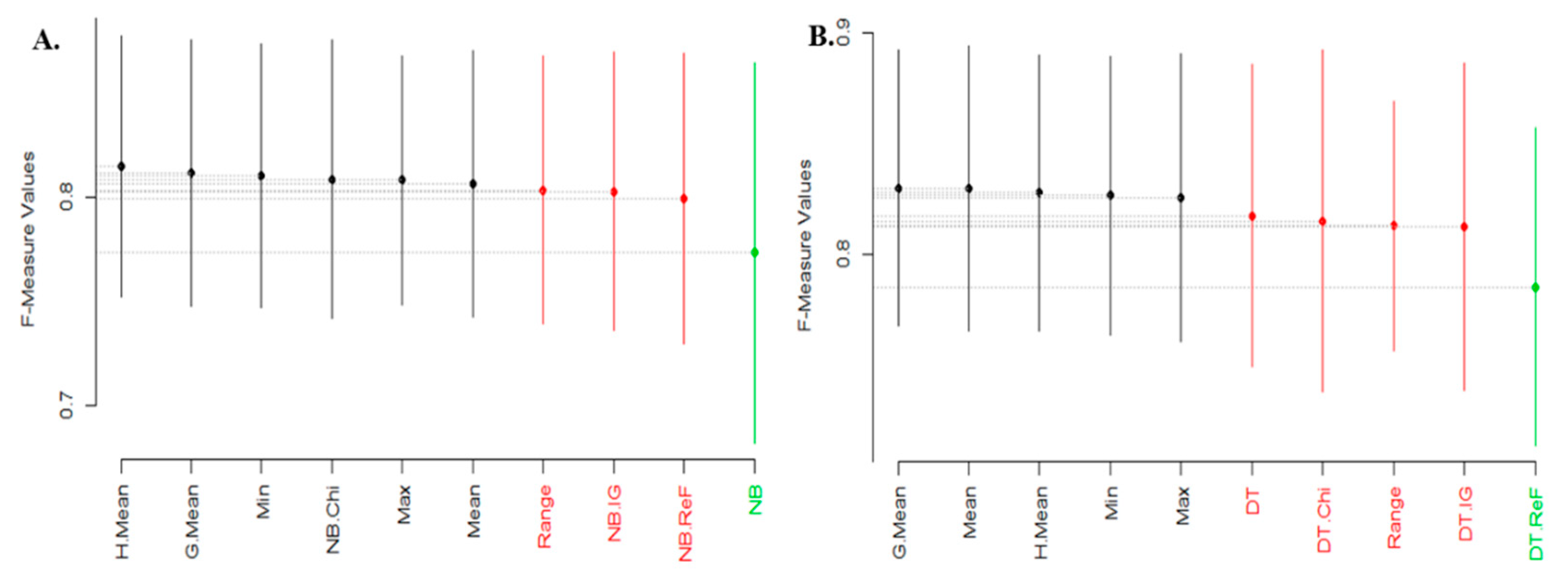
Statistical Rank	Average Accuracy		Average AUC		Average F-Measure
	NB	DT	NB	DT	NB	DT
1	HMean, Min, GMean, Max, Mean, Range, NB + REF	GMean, Mean, HMean, Max, Min, DT + CS, Range, DT + IG	Min, HMean, GMean, Max, Mean	GMean, Min, Max, HMean, Mean	HMean, GMean, Min, NB + CS, Max, Mean	GMean, Mean, HMean, Min, Max
2	NB + CS, NB + IG	DT + REF, DT	NB + REF, NB + IG, NB + CS, Range	Range, DT + CS	Range, NB + IG, NB + REF	DT, DT + CS, Range, DT + IG
3	NB	-	NB	DT + IG	NB	DT + REF
4	-	-	-	DT	-	-
5	-	-	-	DT + REF	-	-

From Figure 5A, concerning average accuracy values, NB models with HMean, Min, GMean, Max, Mean, Range-based RMFFS methods and NB + REF fall into the same category. These set of models are superior in performance and there are statistically significant differences in their means to other NB models. NB + CS and NB + IG models rank second while NB model with NO FS method ranks third. Additionally, from Figure 5B, DT models with GMean, Mean, HMean, Max, Min, DT + CS, Range, DT + IG are statistically superior and ranks higher than DT + REF and DT models. Additionally, the ordering of models from the statistical rank test is important and models which appear first (from left to right) are superior to the other models regardless of their groupings. Similarly, based on average AUC values as presented in Figure 6, NB models with Min, HMean, GMean, Max, Mean-based RMFFS ranks first, while NB + REF, NB + IG, NB + CS and Range-based RMFFS ranks second and NB with no FS method ranks last. DT models GMean, Min, Max, HMean, Mean-based RMFFS ranks first, Range-based RMFFS and DT + CS ranks second, DT + IG ranks third, DT with no FS methods ranks fourth and DT + REF ranks fifth.

Lastly, Figure 7 presents the Scott-Knott rant test results using average f-measure values. NB models with HMean, GMean, Min, NB + CS, Max, Mean-based RMFFS are superior and ranks first while NB models based on Range RMFFS, NB + IG and NB + REF ranks second and NB with NO FS method came last. DT models with GMean, Mean, HMean, Min and Max-based RMFFS ranks first, DT with NO FS method, DT + CS, Range-based RMFFS and DT + IG ranks second while DT + REF ranks third. Table 6 summarizes the analysis of the Scott-Knott Rank Test of experimented FS methods on NB and DT models.

Summarily, from the experimental results and statistical test, the proposed RMFFS methods recorded superior positive impact on the prediction performances of SDP models (NB and DT) than individual FSS (IG, REF and CS) methods on the studied defect datasets. Whereas, the GMean-based RMFFS method outperforms all experimented FS methods. These findings, therefore, answers RQ1 and RQ2 (see Section 3.6) as presented in Table 7. Additionally, the effectiveness of RMFFS addresses filter selection problem by combining the strength of individual filter FS methods in SDP. Hence, it is recommended as a viable option to combine filter (multi-filter) methods to harness the strength of respective FFS and capabilities of filter-filter relationships in selecting germane features for during FS methods as conducted in this study.

Table 7. Answers to Research Questions.

Research Questions	Answers
RQ1. How effective are the proposed RMFFS methods compared to individual filter FS methods?	The proposed RMFFS outperforms individual FFS methods with significant differences.
RQ2. Which of RMFFS methods had the highest positive impact on the prediction performance of SDP models?	GMean-based RMFFS method was superior to other RMFFS methods.

5. Conclusions

This study addresses high dimensionality and filter selection problems in software defect prediction by proposing novel rank aggregation-based Multi-Filter Feature Selection Methods (RMFFS). The selection of an appropriate filter rank method is often a hard choice as the performance of filter methods depends on datasets and classifier used. Consequently, RMFFS combines individual rank lists generated by independent FFS methods from the software defect dataset into a single rank list based on rank aggregation methods. Additionally, a geometric mean function was used to automatically select top-ranked features from the aggregated list. For assessment, features generated by RMFFS and other experimented filter methods (IG, CS, REF and No FS method) were applied with NB and DT classifiers on software defect datasets from NASA repository. Analysis from the experimental results showed the effectiveness and superiority of RMFFS methods as they had a superior positive impact on the prediction performances of NB and DT classifiers than other experimented FS methods in most cases. That is, the proposed RMFFS was able to generate a more stable and complete subset of features that best represent studied datasets. Hence, this makes the combining of individual filter rank methods a viable solution to the filter rank selection problem and enhancement of prediction models in SDP. In a broader perspective, findings from this study can be used in experts and researchers in SDP and other applicable research domains that require FS methods as a method of address high dimensionality and filter selection problem.

As a limitation to this study, we intend to explore and extend the scope of this study by investigating other ensemble configurations of FS method with more prediction models as future works. Additionally, the effect of threshold values on the efficacies of FFS is worth investigating as the adequate threshold value to an extent relies on the used dataset.

References

- Afzal, W.; Torkar, R. Towards benchmarking feature subset selection methods for software fault prediction. In Computational Intelligence and Quantitative Software Engineering; Springer: Berlin/Heidelberg, Germany, 2016; pp. 33–58. [Google Scholar]
- Akintola, A.G.; Balogun, A.O.; Lafenwa-Balogun, F.; Mojeed, H.A. Comparative analysis of selected heterogeneous classifiers for software defects prediction using filter-based feature selection methods. FUOYE J. Eng. Technol. 2018, 3, 134–137. [Google Scholar] [CrossRef]
- Basri, S.; Almomani, M.A.; Imam, A.A.; Thangiah, M.; Gilal, A.R.; Balogun, A.O. The Organisational Factors of Software Process Improvement in Small Software Industry: Comparative Study. In Proceedings of the International Conference of Reliable Information and Communication Technology, Johor, Malaysia, 22–23 September 2019; Springer: Berlin/Heidelberg, Germany, 2019; pp. 1132–1143. [Google Scholar]
- Bajeh, A.O.; Oluwatosin, O.-J.; Basri, S.; Akintola, A.G.; Balogun, A.O. Object-Oriented Measures as Testability Indicators: An Empirical Study. J. Eng. Sci. Technol. 2020, 15, 1092–1108. [Google Scholar]
- Balogun, A.; Bajeh, A.; Mojeed, H.; Akintola, A. Software defect prediction: A multi-criteria decision-making approach. Niger. J. Technol. Res. 2020, 15, 35–42. [Google Scholar] [CrossRef]
- Chauhan, A.; Kumar, R. Bug Severity Classification Using Semantic Feature with Convolution Neural Network. In Computing in Engineering and Technology; Springer: Berlin/Heidelberg, Germany, 2020; pp. 327–335. [Google Scholar]
- Jimoh, R.; Balogun, A.; Bajeh, A.; Ajayi, S. A PROMETHEE based evaluation of software defect predictors. J. Comput. Sci. Its Appl. 2018, 25, 106–119. [Google Scholar]
- Catal, C.; Diri, B. Investigating the effect of dataset size, metrics sets, and feature selection techniques on software fault prediction problem. Inf. Sci. 2009, 179, 1040–1058. [Google Scholar] [CrossRef]
- Li, L.; Leung, H. Mining static code metrics for a robust prediction of software defect-proneness. In Proceedings of the 2011 International Symposium on Empirical Software Engineering and Measurement, Washington, DC, USA, 22–23 September 2011; pp. 207–214. [Google Scholar]
- Mabayoje, M.A.; Balogun, A.O.; Bajeh, A.O.; Musa, B.A. Software Defect Prediction: Effect of feature selection and ensemble methods. FUW Trends Sci. Technol. J. 2018, 3, 518–522. [Google Scholar]
- Lessmann, S.; Baesens, B.; Mues, C.; Pietsch, S. Benchmarking classification models for software defect prediction: A proposed framework and novel findings. IEEE Trans. Softw. Eng. 2008, 34, 485–496. [Google Scholar] [CrossRef]
- Li, N.; Shepperd, M.; Guo, Y. A systematic review of unsupervised learning techniques for software defect prediction. Inf. Softw. Technol. 2020, 122, 106287. [Google Scholar] [CrossRef]
- Okutan, A.; Yıldız, O.T. Software defect prediction using Bayesian networks. Empir. Softw. Eng. 2014, 19, 154–181. [Google Scholar] [CrossRef]
- Rodriguez, D.; Herraiz, I.; Harrison, R.; Dolado, J.; Riquelme, J.C. Preliminary comparison of techniques for dealing with imbalance in software defect prediction. In Proceedings of the 18th International Conference on Evaluation and Assessment in Software Engineering, London, UK, 13–14 May 2014; pp. 1–10. [Google Scholar]
- Usman-Hamza, F.; Atte, A.; Balogun, A.; Mojeed, H.; Bajeh, A.; Adeyemo, V. Impact of feature selection on classification via clustering techniques in software defect prediction. J. Comput. Sci. Its Appl. 2019, 26. [Google Scholar] [CrossRef]
- Balogun, A.; Oladele, R.; Mojeed, H.; Amin-Balogun, B.; Adeyemo, V.E.; Aro, T.O. Performance analysis of selected clustering techniques for software defects prediction. Afr. J. Comp. ICT 2019, 12, 30–42. [Google Scholar]
- Rodriguez, D.; Ruiz, R.; Cuadrado-Gallego, J.; Aguilar-Ruiz, J.; Garre, M. Attribute selection in software engineering datasets for detecting fault modules. In Proceedings of the 33rd EUROMICRO Conference on Software Engineering and Advanced Applications (EUROMICRO 2007), Lubeck, Germany, 28–31 August 2007; pp. 418–423. [Google Scholar]
- Wang, H.; Khoshgoftaar, T.M.; van Hulse, J.; Gao, K. Metric selection for software defect prediction. Int. J. Softw. Eng. Knowl. Eng. 2011, 21, 237–257. [Google Scholar] [CrossRef]
- Rathore, S.S.; Gupta, A. A comparative study of feature-ranking and feature-subset selection techniques for improved fault prediction. In Proceedings of the 7th India Software Engineering Conference, Chennai, India, 19–21 February 2014; pp. 1–10. [Google Scholar]
- Xu, Z.; Liu, J.; Yang, Z.; An, G.; Jia, X. The impact of feature selection on defect prediction performance: An empirical comparison. In Proceedings of the 2016 IEEE 27th International Symposium on Software Reliability Engineering (ISSRE), Ottawa, ON, Canada, 23–27 October 2016; pp. 309–320. [Google Scholar]
- Balogun, A.O.; Shuib, B.; Abdulkadir, S.J.; Sobri, A. A Hybrid Multi-Filter Wrapper Feature Selection Method for Software Defect Predictors. Int. J Sup. Chain. Manag. 2019, 8, 916. [Google Scholar]
- Balogun, A.O.; Basri, S.; Abdulkadir, S.J.; Hashim, A.S. Performance Analysis of Feature Selection Methods in Software Defect Prediction: A Search Method Approach. Appl. Sci. 2019, 9, 2764. [Google Scholar] [CrossRef]
- Balogun, A.O.; Basri, S.; Mahamad, S.; Abdulkadir, S.J.; Almomani, M.A.; Adeyemo, V.E.; Al-Tashi, Q.; Mojeed, H.A.; Imam, A.A.; Bajeh, A.O.; et al. Impact of Feature Selection Methods on the Predictive Performance of Software Defect Prediction Models: An Extensive Empirical Study. Symmetry 2020, 12, 1147. [Google Scholar] [CrossRef]
- Ghotra, B.; McIntosh, S.; Hassan, A.E. A large-scale study of the impact of feature selection techniques on defect classification models. In Proceedings of the 2017 IEEE/ACM 14th International Conference on Mining Software Repositories (MSR), Piscataway, NJ, USA, 20–21 May 2017; pp. 146–157. [Google Scholar]
- Anbu, M.; Mala, G.A. Feature selection using firefly algorithm in software defect prediction. Clust. Comput. 2019, 22, 10925–10934. [Google Scholar] [CrossRef]
- Kakkar, M.; Jain, S. Feature selection in software defect prediction: A comparative study. In Proceedings of the 6th International Conference on Cloud System and Big Data Engineering, Noida, India, 14–15 January 2016; pp. 658–663. [Google Scholar]
- Cai, J.; Luo, J.; Wang, S.; Yang, S. Feature selection in machine learning: A new perspective. Neurocomputing 2018, 300, 70–79. [Google Scholar] [CrossRef]
- Li, Y.; Li, T.; Liu, H. Recent advances in feature selection and its applications. Knowl. Inf. Syst. 2017, 53, 551–577. [Google Scholar] [CrossRef]
- Chandrashekar, G.; Sahin, F. A survey on feature selection methods. Comput. Electr. Eng. 2014, 40, 16–28. [Google Scholar] [CrossRef]
- Iqbal, A.; Aftab, S. A Classification Framework for Software Defect Prediction Using Multi-filter Feature Selection Technique and MLP. Int. J. Mod. Educ. Comput. Sci. 2020, 12, 18–25. [Google Scholar] [CrossRef]
- Osanaiye, O.; Cai, H.; Choo, K.-K.R.; Dehghantanha, A.; Xu, Z.; Dlodlo, M. Ensemble-based multi-filter feature selection method for DDoS detection in cloud computing. EURASIP J. Wirel. Commun. Netw. 2016, 2016, 130. [Google Scholar] [CrossRef]
- Cynthia, S.T.; Rasul, M.G.; Ripon, S. Effect of Feature Selection in Software Fault Detection. In Proceedings of the International Conference on Multi-disciplinary Trends in Artificial Intelligence, Kuala Lumpur, Malaysia, 17–19 November 2019; Springer: Berlin/Heidelberg, Germany, 2019; pp. 52–63. [Google Scholar]
- Jia, L. A hybrid feature selection method for software defect prediction. IOP Conf. Ser. Mater. Sci. Eng. 2018, 394, 032035. [Google Scholar] [CrossRef]
- Jacquier, E.; Kane, A.; Marcus, A.J. Geometric or arithmetic mean: A reconsideration. Financ. Anal. J. 2003, 59, 46–53. [Google Scholar] [CrossRef]
- Wang, H.; Khoshgoftaar, T.M.; Napolitano, A. A comparative study of ensemble feature selection techniques for software defect prediction. In Proceedings of the 2010 Ninth International Conference on Machine Learning and Applications, Washington, DC, USA, 12–14 December 2010; IEEE: Washington, DC, USA, 2010; pp. 135–140. [Google Scholar]
- Xia, Y.; Yan, G.; Jiang, X.; Yang, Y. A new metrics selection method for software defect prediction. In Proceedings of the 2014 IEEE International Conference on Progress in Informatics and Computing, Shanghai, China, 16–18 May 2014; IEEE: Shanghai, China, 2014; pp. 433–436. [Google Scholar]
- Malik, M.R.; Yining, L.; Shaikh, S. The Role of Attribute Ranker using classification for Software Defect-Prone Data sets Model: An Empirical Comparative Study. In Proceedings of the 2020 IEEE International Systems Conference (SysCon), Montreal, QC, Canada, 24 August–20 September 2020; pp. 1–8. [Google Scholar]
- Yu, Q.; Jiang, S.; Zhang, Y. The performance stability of defect prediction models with class imbalance: An empirical study. IEICE TRANS. Inf. Syst. 2017, 100, 265–272. [Google Scholar] [CrossRef]
- Shepperd, M.; Song, Q.; Sun, Z.; Mair, C. Data quality: Some comments on the NASA software defect datasets. IEEE Trans. Softw. Eng. 2013, 39, 1208–1215. [Google Scholar] [CrossRef]
- Balogun, A.O.; Lafenwa-Balogun, F.B.; Mojeed, H.A.; Adeyemo, V.E.; Akande, O.N.; Akintola, A.G.; Bajeh, A.O.; Usman-Hamza, F.E. SMOTE-Based Homogeneous Ensemble Methods for Software Defect Prediction. In Proceedings of the International Conference on Computational Science and Its Applications, Cagliari, Italy, 1–4 July 2020; Springer: Berlin/Heidelberg, Germany, 2020; pp. 615–631. [Google Scholar]
- Balogun, A.O.; Bajeh, A.O.; Orie, V.A.; Yusuf-Asaju, W.A. Software Defect Prediction Using Ensemble Learning: An ANP Based Evaluation Method. FUOYE J. Eng. Technol. 2018, 3, 50–55. [Google Scholar] [CrossRef]
- Imam, A.A.; Basri, S.; Ahmad, R.; Wahab, A.A.; González-Aparicio, M.T.; Capretz, L.F.; Alazzawi, A.K.; Balogun, A.O. DSP: Schema Design for Non-Relational Applications. Symmetry 2020, 12, 1799. [Google Scholar] [CrossRef]
- James, G.; Witten, D.; Hastie, T.; Tibshirani, R. An Introduction to Statistical Learning; Springer: Berlin/Heidelberg, Germany, 2013. [Google Scholar]
- Kuhn, M.; Johnson, K. Applied Predictive Modelling; Springer: Berlin/Hedielberg, Germany, 2013. [Google Scholar]
- Alsariera, Y.A.; Adeyemo, V.E.; Balogun, A.O.; Alazzawi, A.K. Ai meta-learners and extra-trees algorithm for the detection of phishing websites. IEEE Access 2020, 8, 142532–142542. [Google Scholar] [CrossRef]
- Alsariera, Y.A.; Elijah, A.V.; Balogun, A.O. Phishing Website Detection: Forest by Penalizing Attributes Algorithm and Its Enhanced Variations. Arab. J. Sci. Eng. 2020, 45, 10459–10470. [Google Scholar] [CrossRef]
- Hall, M.; Frank, E.; Holmes, G.; Pfahringer, B.; Reutemann, P.; Witten, I.H. The WEKA Data Mining Software: An Update. ACM SIGKDD Explor. Newsl. 2009, 11, 10–18. [Google Scholar] [CrossRef]
- Tantithamthavorn, C.; McIntosh, S.; Hassan, A.E.; Matsumoto, K. Comments on “Researcher Bias: The Use of Machine Learning in Software Defect Prediction”. IEEE Trans. Softw. Eng. 2016, 42, 1092–1094. [Google Scholar] [CrossRef]
- Tantithamthavorn, C.; McIntosh, S.; Hassan, A.E.; Matsumoto, K. The Impact of Automated Parameter Optimization on Defect Prediction Models. IEEE Trans. Softw. Eng. 2018, 45, 683–711. [Google Scholar] [CrossRef]