PSO Based Optimized Ensemble Learning and Feature Selection Approach for Efficient Energy Forecast

Abstract

Swarm intelligence techniques with incredible success rates are broadly used for various irregular and interdisciplinary topics. However, their impact on ensemble models is considerably unexplored. This study proposes an optimized-ensemble model integrated for smart home energy consumption management based on ensemble learning and particle swarm optimization (PSO). The proposed model exploits PSO in two distinct ways; first, PSO-based feature selection is performed to select the essential features from the raw dataset. Secondly, with larger datasets and comprehensive range problems, it can become a cumbersome task to tune hyper-parameters in a trial-and-error manner manually. Therefore, PSO was used as an optimization technique to fine-tune hyper-parameters of the selected ensemble model. A hybrid ensemble model is built by using combinations of five different baseline models. Hyper-parameters of each combination model were optimized using PSO followed by training on different random samples. We compared our proposed model with our previously proposed ANN-PSO model and a few other state-of-the-art models. The results show that optimized-ensemble learning models outperform individual models and the ANN-PSO model by minimizing RMSE to 6.05 from 9.63 and increasing the prediction accuracy by 95.6%. Moreover, our results show that random sampling can help improve prediction results compared to the ANN-PSO model from 92.3% to around 96%.

1. Introduction

Due to the ever-escalating world’s population, energy consumption and its demand have also increased at an accelerated rate over the past few years [1]. According to the authors of [2], the energy demands for the residential building segment are expected to rise by 70%. Additionally, in the U.S., industrial and domestic buildings collectively consumed 74% of the total electricity generated in 2015 [3]. However, efficient energy management for households is of vital importance as this sector has a substantial possibility for energy saving compared to other industries [4]. Efficient energy management refers to optimally minimizing the energy consumption without affecting users’ comfort and daily tasks such as cooling, heating, ventilating, and other operations.

Artificial intelligence (AI) based techniques have played a significant role in efficient energy forecasting tasks. Many popular approaches have been considered previously, such as Artificial Neural Networks (ANNs), Support Vector Regression (SVR), Long-Short Term Memory networks (LSTMs), etc. Jain et al. used the SVM algorithm to predict multi-family residential buildings’ energy consumption in urban environments [5]. Howard et al. used multivariate linear regression to analyze the building energy end-use intensities in New York City [6]. ANNs have also been applied in initial design stages to enhance the prediction of energy utilization for residential buildings. In our previous study based on a hybrid approach, ANN has a vital role in optimal energy consumption forecasting [7].

Though established to bring few advancements and improvements over conventional statistical approaches, AI models have their own inadequacies and drawbacks. For example, issues like overfitting and local minima in ANN and sensitiveness to parameter selection in both SVR and ANN models. Given the limitations of traditional techniques and AI techniques for energy consumption forecasting, a novel approach is required for challenging forecasting tasks with high volatility and irregularity.

In this paper, based on the concept of decomposition and ensemble introduced by Yu [8], we have proposed a hybrid optimized-ensemble model that utilizes the strengths of the Particle Swarm Optimization (PSO) algorithm. As the name suggests, decomposition aims to simplify the complicated prediction tasks by dividing them into comparatively manageable sub-tasks; ensemble, on the other hand, considers multiple models and formulates prediction results. The proposed optimized-ensemble model aptly takes one step further after developing different ensemble combinations to optimize the results and find the optimal combination of models using PSO. We have performed random sampling on data before using it for the training and generated different subsamples of data. Random sampling was done to find the best sample size for training. To eliminate the risks of overfitting and multi-collinearity, we performed a PSO-based feature selection before developing the optimized-ensemble model and formulated an objective function for significant variables. We have used CatBoost, XGBoost, LightBoost, RandomForest, and GradientBoosting for ensemble modeling in various combinations. To explain the proposed methodology’s sufficiency, we analyzed the effects of feature selection and compared the predictive power between the proposed ensemble models and individual models. The main contributions of this study are as follows:

(i)

The proposed optimized-ensemble model is a hybrid that consists of random sampling, feature selection, and ensemble learning.

(ii)

In the proposed study, the use of PSO is two-fold; it both helps in feature selection and for achieving optimal prediction results among different ensemble combinations by using it to optimize hyper-parameters. We refer to it as an optimized-ensemble model.

(iii)

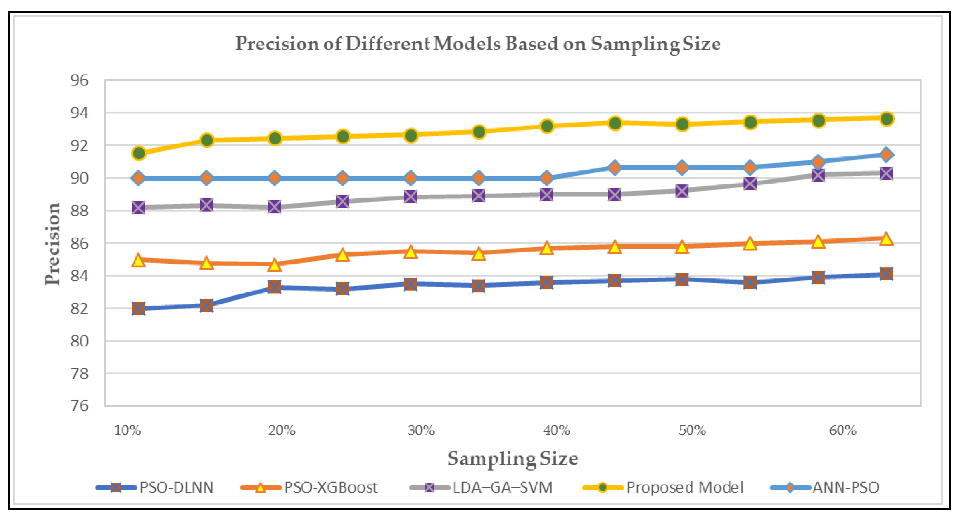
The effectiveness of the proposed optimized-ensemble model is compared to different individual models, varying models of the ensemble, and the previously proposed method, i.e., ANN-PSO. The results show that optimized ensemble has better performance than non-optimized ensemble, individual models, and previously presented models.

The remainder of this paper is organized as follows: Section 2 discusses the related works; Section 3 reviews the overall proposed methodology, and Section 4 presents implementation setup. The experiment results are presented in Section 5; Section 6 discusses the significant findings and limitations and concludes.

2. Related Works

This section presents related literature studies and is further divided into subsections. Section 2.1 presents and compares some general studies that have focused on energy consumption prediction using three different approaches. Section 2.2 presents a literature review of PSO-based feature selection approaches and Section 2.3 highlights approaches to tune and optimize hyper-parameters of different models.

2.1. Energy Consumption Forecasting Techniques

The methods used for forecasting involve different approaches such as machine learning-based approaches, non-machine learning-based approaches, ensemble machine learning-based approaches, etc. In Table 1, we have presented a summary of the pros and cons of each type of approach used for energy consumption forecasting. In the case of the non-machine learning model, the most frequently used techniques include linear regression [9], statistical methods [10], rule-based approaches [11], etc. However, due to their limitations, these approaches might not yield satisfactory results for energy forecasting in smart buildings. For optimal energy consumption forecasting, there is a need to train large, multi-dimensional, and historical data. That is why deep learning approaches are considered to yield satisfactory results in such scenarios.

Table 1. Common characteristics of classical (non-machine learning-based), individual, and ensemble ML models.

Techniques	Strengths	Weakness
Classical Methods	- Traditional and well known in the literature. - Can offer statistical implications of prediction. - Generally, these methods can measure uncertainty or ambiguity in predictions. - Provide easy and quick implementation for any problem at hand.	- These models can poorly perform in predicting short-term time series. - Element of unreliability exists due to reliance upon different assumptions. - These prediction models possess a restricted capacity to deal with supplementary variables. - The curse of dimensionality exists.
Individual Machine Learning Methods	- No assumptions are required for variables. - Show better performance and flexible nature to handle time series. - Additional variables can be accommodated easily in time-series predictions. - As compared to classical models, these models have effective generalization capability.	- It might have a higher computational cost as compared with classical methods. - Lack of understanding and explanation of fitting nature of different models. - The curse of dimensionality also exists. - Characteristic uncertainty in the learning and training, though observing and dealing with similar patterns.
Ensemble Machine Learning Methods	- Highly flexible and best fitting approaches. - Show higher stability in performance individual ML models. - Uncertainty can be explained. - Effectively minimizes the curse of dimensionality.	- It is a comparatively new approach. - It might be computationally costly in some cases. - It is still developing for regression-related problems. - Careful consideration is required to apply generic models to a specific field of study.

Several studies have suggested deep learning-based solutions for energy prediction, such as using SVMs [12], ANNs [13], Decision Trees (DTs) [14], LSTM [15], etc. Numerous studies have proved that machine learning models can substantially outperform state-of-the-art statistical models [16]. Salgado in [17] has proposed a DT-based hybrid approach to predict energy load. The model uses climate information to calculate the load. In [18], Li et al. have established an SVM-based prediction method for energy usage prediction in domestic buildings. In addition, in [19], SVMs and ANN-based models are reviewed for household energy consumption prediction. In a more specific study [20], an ANN-based forecasting tool is implemented to predict energy forecasts in a building. Here, nine different scenarios are considered, and different ANNs are developed according to a scenario. Despite many machine learning models in household energy prediction, there are still some challenges, such as misleading patterns. Therefore, specific model’s optimization can generate distinct patterns indicating that such unstable behaviors might negatively affect the generalization capability of ML models if there are different patterns or conditions observed in the training and validation data. Comparatively, ensemble learning happens to be a widely appreciated improvement to standard ML approaches. Thus, it is recommended over an extensive range of applications in different research studies [21,22,23].

Compared to individual models, the primary benefits of utilizing an ensemble model are portrayed in their enhanced generalization capability and adaptable, functional mapping among the system’s variables. The ensemble models are of two different kinds; homogenous models are usually an ensemble of similar processes; heterogeneous models consist of an ensemble of other techniques and are also known as hybrid models.

Ensemble learning is getting popular in the energy forecast domain as well. In [24], an ensemble bagging tree approach (EBT) is presented to forecast building electricity demand. Yang in [25] has proposed a deep ensemble learning-based load forecasting model, an end-to-end probabilistic model. It is a least absolute shrinkage and selection operator-based quantile prediction approach for deep ensemble learning framework.

2.2. PSO-Based Feature Selection

Feature selection is a critical preprocessing task in classification that eliminates irrelevant, redundant, and noisy features. Improving the model’s performance, decreasing the computational cost, and adjusting the “curse of dimensionality” are the key advantages of the feature selection task.

Optimal feature selection can play a significant role in accurate forecasting as using raw features may lead to an inefficient result. Therefore, many approaches use different feature selection methods to prepare their data to train the model. In [26], a new process is proposed where threshold based binary PSO is used for feature selection to enhance the performance of the face-recognition system. In another study [27], a PSO-based hybrid approach selects relevant features from raw features. A study in [28] presents the exploratory aftereffect of organization irregularity discovery utilizing PSO for feature selection and ensemble learning-based model that uses tree-based classifiers (C4.5, Random Forest, and CART) for classification. The proposed recognition model shows a promising outcome with recognition precision and a lower positive rate than existing ensemble methods. Another variation of the PSO-based feature selection technique is presented in [29] that utilizes features frequency for feature elitism. In [30], a new PSO-based multi-objective feature selection technique is presented. In this technique, raw features are considered a graph model, and the centralities for all the nodes are calculated, and a PSO-based search process is performed to select the final set of features.

2.3. PSO for Hyper-Parameter Optimization

Hyper-parameter tuning has been of great importance for learning algorithms as it can extensively affect their model optimization. Initially, hyper-parameter tuning was performed by using simple yet exhaustive approaches e.g., grid search and random search [31]. Unfortunately, these methods suffer from issues such as search space complexity and high variance [32]. Besides this, some other strategies for optimization were proposed such as sequential model-based optimization [33] and Bayesian optimization [34]. This has been a significant obstacle in deep neural networks (DNNs). Many studies have been proposed that use PSO to optimize hyper-parameters of DNNs. In [35], PSO proves to generate promising classification accuracy by efficiently exploring the solution space. In [36], a parallel method is introduced where the PSO’s population is evolved in parallel to their fitness evaluation. A novel variation of PSO named as cPSO-CNN in [37], aims to enhance CNN hyper-parameter tuning process and utilize a normal distribution-based confidence function. Similarly, several other works [38,39] are performed for DNNs to optimize the hyper-parameters. However, for ensemble models this task is quite challenging and with different settings and objectives the optimization goal of a model can change. In a recent study [40] a stacked ensemble model for software effort estimation used both GA and PSO are optimized hyper-parameters. In [41], a cascade swarm intelligence algorithm is proposed for image segmentation that also uses PSO for tuning hyper-parameters of deep CNNs.

In this study, we have proposed a dual-purpose PSO-based ensemble learning model used for feature selection and optimization by tuning the hyper-parameters of the ensemble model.

3. Proposed Methodology

In this section, we introduce our proposed methodology in detail. In Section 3.1, we present the conceptual view of this research. Section 3.2 introduces the detailed architecture of the system. This section is further divided into multiple subsections. Each subsection sheds some light on individual modules of the overall architecture including the hybrid ensemble model in detail with various subsections.

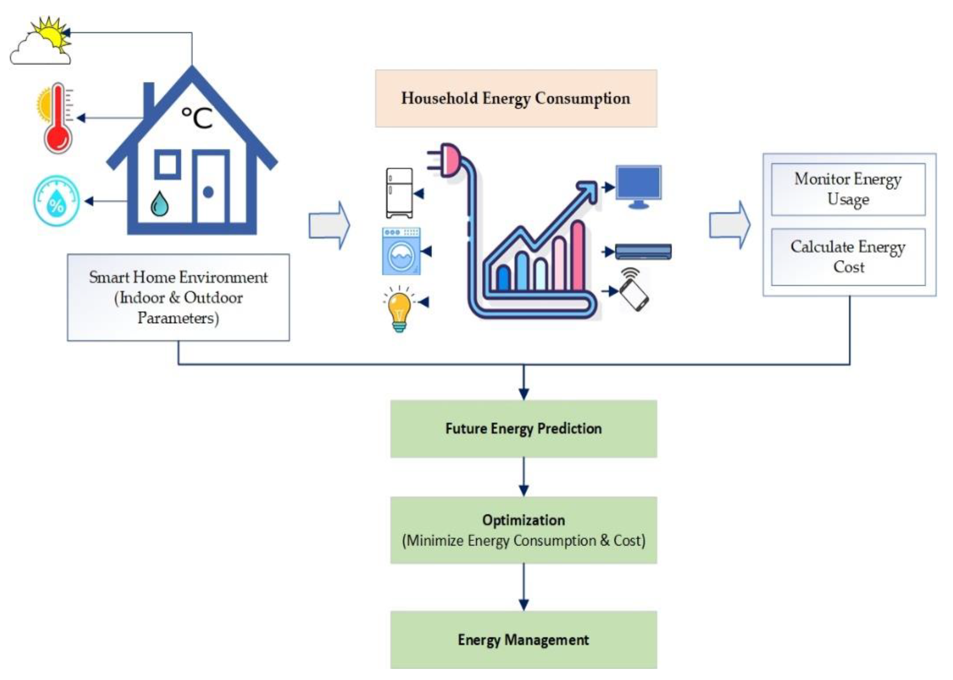
3.1. Conceptual View

This section presents a basic conceptual flow and abstract view of this research work in Figure 1. The simple idea is to manage the energy consumption of smart homes based on their energy usage patterns and forecasting to reduce energy costs. Energy consumption in a household depends on multiple factors, such as outdoor weather conditions, indoor environment, number of appliances and their usage frequency, etc.

Figure 1. Conceptual view of the system.

Therefore, outdoor parameters such as temperature, humidity, and weather conditions are considered, along with indoor parameters and the overall energy consumption. The data is trained to get the future energy consumption predictions and based on these predictions we aim to manage the energy inside a house by generating different control rules for various appliances.

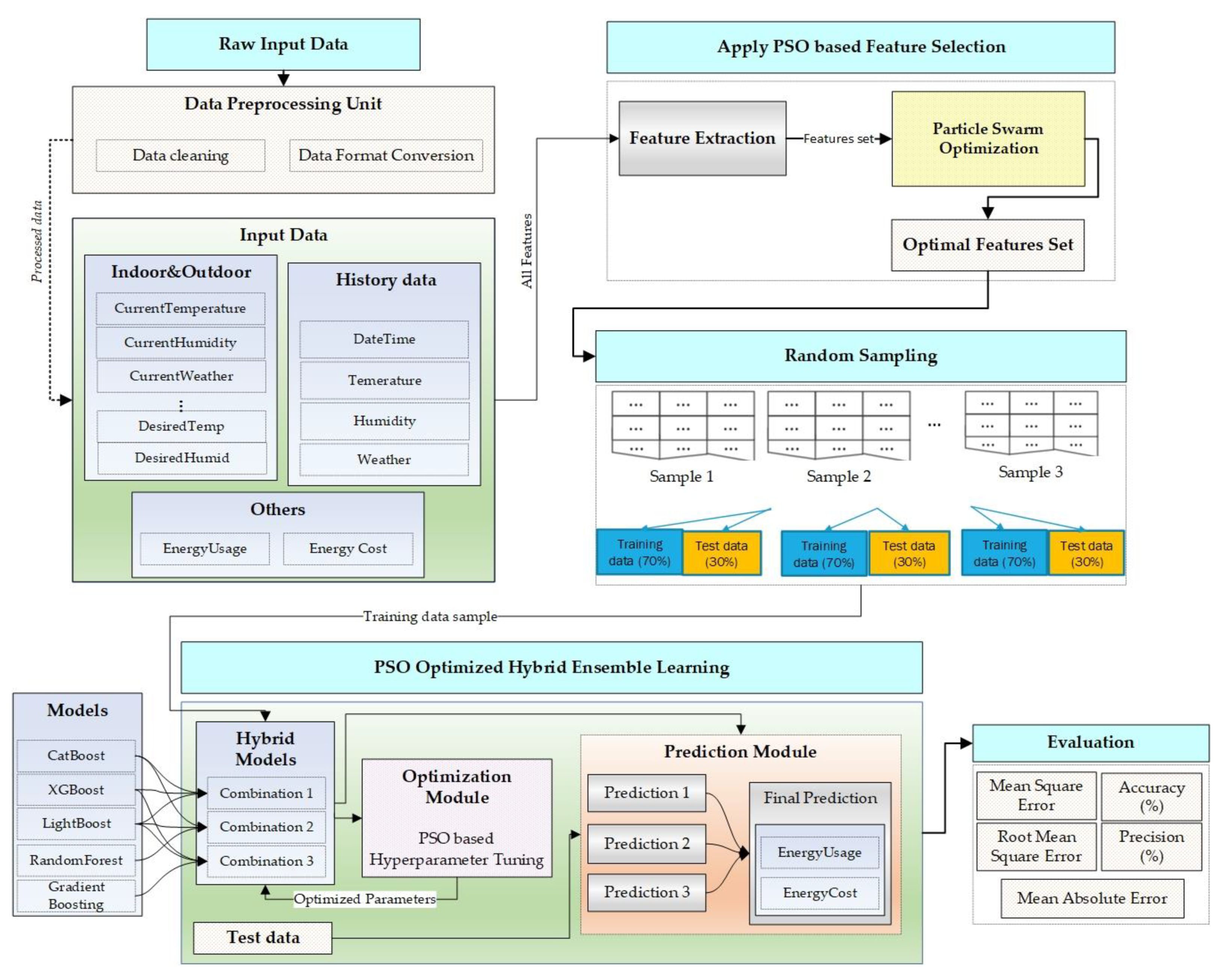
3.2. Architectural View

This section presents the architectural details of the proposed model. The proposed model integrates multiple modules, and each module plays a significant role in achieving the desired objective. As shown in Figure 2, there are five primary modules such as data module, a feature selection module, random sampling module, ensemble learning module, and evaluation module.

Figure 2. Overall architectural view of the proposed system.

The data module handles raw data, preprocesses it, and prepares a features list from all the relevant parameters. The feature selection module is based on PSO that uses the features list as input and returns an optimized set of features based on their respective scores calculated using the Gaussian Mixture Model (GMM). The random sampling module takes all the data based on essential and optimized elements and generates different random samples of data. Each random sample is trained separately. The most crucial module is our hybrid ensemble learning module, which again uses PSO for optimization by tuning the hyper-parameters of all the models. The last module is the evaluation module that uses different evaluation metrics to assess the performance of all the models.

3.2.1. Data

The data is comprised of both indoor and outdoor parameters such as temperature (indoor, outdoor), humidity (indoor, outdoor), weather, timestamp, dew point, energy consumption, energy consumption cost, precipitation, user desired ranges of temperature and humidity, etc. The timestamp column was decomposed into eight new columns such as hour, year, month, quarter, day of year, day of month, day of week, and week of year. We performed feature selection on a total of 20 columns in the input dataset. According to fitness estimation in PSO algorithm, the total number of selected features were 10. The selected features were indoor temperature, outdoor temperature, indoor humidity, outdoor humidity, energy consumption, energy consumption cost, month, weather, dew point, and precipitation. Figure 3 presents the fitness graph and feature size for our input dataset. We have divided the dataset into 70% training data, 10% validation, and 20% test data for our proposed model.

Figure 3. Fitness estimation through PSO feature selection.

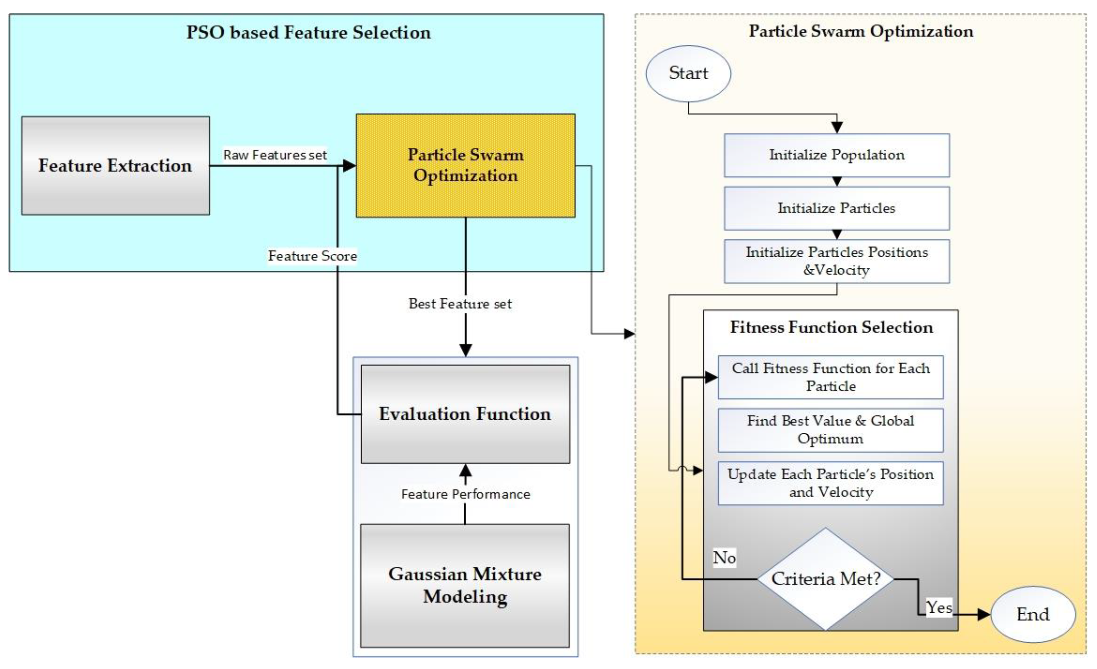
3.2.2. PSO-Based Feature Selection

Feature selection is the method for choosing a subgroup of significant features to construct a model. It aims to enhance the data quality by selecting the best features for the model performance. The process of feature selection by using PSO is shown in Figure 4.

Figure 4. PSO-based feature selection.

We have used a variation of the binary particle swarm optimization (BPSO) algorithm, which primarily is a binary version of PSO [42]. The primary functions are the same as PSO; in BPSO, both local best (pbest) and global best (gbest) solutions exist. Here, the positions of the particles are stated in two terms, i.e., 0 (not selected) and 1 (preferred). The position and velocity of a particle on d-dimensions at any given time t can be defined in Equations (1) and (2).

$$x_i^d\left(t+1\right)=x_1\left(t\right),x_2\left(t\right),x_3\left(t\right),\dots x_d\left(t\right)x_iƐ0,1$$

(1)

$$v_i^d\left(t+1\right)=w{v}_i^d\left(\mathrm{t}\right)+c_{1}ran{d}_1\left(pbes{t}_i^d\left(t\right)-x_i^d\left(t\right)\right)+c_{2}ran{d}_2\left(gbes{t}_i^d\left(t\right)-x_i^d\left(t\right)\right)$$

(2)

where $x_i$ is the position of a particle; $v_i$ is the velocity of the particle; acceleration factors are represented as $c_1$ and $c_2$; $ran{d}_1$ and $ran{d}_2$ represents two random numbers in the range [0,1]; d refers to the dimension in the search space, and t is the number of iterations.

For each particle, its velocity is updated and changed to probability. Additionally, the position of the particle is updated based on its updated velocity. The position and velocity of a particle can be updated by using Equations (3) and (4).

$$V_{update(v_i^d\left(t+1\right))}=\frac{1}{1+\exp -v_i^d\left(t+1\right)}$$

(3)

$$P_{update(x_i^d\left(t+1\right)}=\{\begin{array}{c}0, if random\ge V_{update(v_i^d\left(t+1\right))} \\ 1, if random<V_{update(v_i^d\left(t+1\right))}\end{array}$$

(4)

where, $V_{update(v_i^d\left(t+1\right))}$ and $P_{update(x_i^d\left(t+1\right)}$ refer to updated velocity and position of a particle, respectively; a random is a random number that has uniformly distributed values between 0 and 1.

The most vital role is played by pbest and gbest values that guide the particles toward the global optimum. Equations (5) and (6) are used to update pbest and gbest values, respectively.

$$pbes{t}_i\left(t+1\right)=\{\begin{array}{c}{x}_i^d\left(t+1\right), if f\left(x_i^d\left(t+1\right)\right)<f\left(x_i^d\left(t\right)\right)\\ pbes{t}_i^d\left(t\right), if f(x_i^d\left(t+1\right)\ge f\left(x_i^d\left(t\right)\right)\end{array}$$

(5)

$$gbes{t}_i\left(t+1\right)=\{\begin{array}{c}pbes{t}_i\left(t+1\right), if f\left(pbes{t}_i\left(t+1\right)\right)<f\left(gbest\left(t\right)\right)\\ gbest\left(t\right), if f(pbes{t}_i\left(t+1\right) \ge f\left(gbest\left(t\right)\right)\end{array}$$

(6)

where x is the position (solution), pbest is the local best solution, gbest is the global best solution, and f(.) is the fitness function defined as in Equation (7).

$$f\left(x\right)=\alpha \left(1-p\right)+\left(1-\alpha \right)(1-\frac{N_{subsetFeatures}}{N_{totalFeatures}})$$

(7)

where α is a hyper-parameter that decides the tradeoff between the classifier performance P, $N_{subsetFeatures}$ refers to the size of features subset, while $N_{totalFeatures}$ represents the total number of features in the dataset. Accuracy, precision, or F-score can be used to evaluate the classifier performance. We have used Gaussian Mixture Modeling for feature evaluation.

Inertia weight, being the most significant parameter in BPSO, handles exploitation and exploration behavior. It is critically essential to achieve a balance between exploitation and exploration. In the literature, several different types of inertia weight strategies are proposed to improve PSO performance. Here, we use our previously proposed velocity-boost-inertia-weight scheme in [43]. We start with a constant inertia weight valuev $II{W}_c$ = 0.729, and a velocity boost threshold (VBT) then, in each iteration, we observe the particle’s pbest, till VBT. If there is no enhancement in the pbest, we assign a new inertia weight to update the particles’ velocities. Based on previously proposed inertia weights in Equation (8) [44] and Equation (9) [45], we define our new inertia weight in Equation (10).

$$InitialInertiaWeigh{t}_{constant}=II{W}_c=0.7$$

(8)

$$RandomInertiaWeigh{t}_{constant}=RIW=0.5+\frac{Rand()}{2}$$

(9)

$$NewInertiaWeigh{t}_{constant}=NIW=II{W}_c+\frac{Rand()}{3}$$

(10)

3.2.3. Random Sampling

We performed random sampling on our dataset to generate different samples of data with different sizes. Random sampling was performed to improve the quality of input data for training, as overfitting might happen when the training data is too large. We experimented with different sample sizes and figured out the most optimal sample size for our model. All these samples were separately used for training. For each random example, we split the data into 70% training, 10% validation, and 20% test data.

We performed random sampling with the reservoir, which is a fast algorithm for selecting a random sample of n records without replacement from a pool of N records, where the value of N is unknown beforehand.

3.2.4. PSO Optimized Hybrid Ensemble Learning Model

The most critical objective of machine learning is to prepare a balanced model that operates perfectly in all circumstances; however, real-life examples and situations are not often ideal. Ensemble learning is the procedure of merging several models to achieve a more comprehensive and better-supervised model. The fundamental idea of ensemble learning is that if a specific weak regressor fails to provide accurate prediction, other regressors can take care of it and improve the results.

We have experimented with a novel machine learning-based hybrid approach, combining multiple combinations of various models such as CatBoost, XGBoost, LightBoost, RandomForest, and GradientBoosting. Then, we randomly selected three different varieties of these models for experiments.

(A)

Hyper-parameter Tuning Using PSO

The hyper-parameters of these combination or hybrid models were optimized using PSO. For any machine learning model with the highest performance, there is a dire need to tune the system for any given problem at hand; otherwise, it will fail to achieve the best performance. It is nearly impossible to adjust the system every time; therefore, manually, automated hyper-parameters tuning diminishes the labor-intensive work for experimenting with various machine learning model configurations. Hyper-parameter tuning enhances the precision of ML algorithms and increases reproducibility. It plays a vital role in producing more accurate results for any ML model [46]. Genetic Algorithms (GA) and PSO are elementary and are discovered to be more efficient in exploring huge hyper-parameter space [47]. However, PSO can obtain the same optimization level as GA but usually with less cost in terms of generations. In Table 2, the critical hyper-parameters for the base learner of ensemble selected are shown along with their value ranges.

Table 2. Hyper-parameters in an ensemble model.

#	Hyper-Parameters	Range
1	Hidden layers size	0–15
2	alpha (L2 regularizer)	0.0001–0.1
3	Number of estimators	0.1–0.8
4	Random state	5–100
5	C(Regularization parameter)	1–100
6	γ (Gamma)	1–300
7	ε (tolerance)	0.01–30

PSO requires several parameters to execute, and all the parameters’ values depend upon the problem. In our case, we are aiming to find optimal deals for all the hyper-parameters. PSO parameters, along with their respective values, are presented in Table 3.

Table 3. PSO parameters set and their corresponding values.

#	Parameters	Values
1	c1 (Local coefficient)	1.5
2	c2 (Global coefficient)	1.5
3	Inertia weight	0.7
4	No. of particles	8
5	Fitness criteria	RMSE

The fitness function depends on the RMSE of the regressor, which should be minimized. Hyper-parameters values are updated in such a way that solution advances toward local best and global best. These hyper-parameter values are then used to update the position of each particle. In each iteration of the algorithm, the fitness condition and the termination condition are verified before calculating pbest and gbest values. As shown in Table 3, RMSE is chosen as fitness criteria, and 200 iterations or RMSE difference among previous iterations <0.3% is selected as the termination criteria. The fitter and finer particles will have a minimum RMSE value for that configuration. The iterations are repeated till the terminal condition is reached, i.e., when the difference of RMSE between two iterations remains <0.3% or the number of iterations exceeds 200. Then the particle with the best fitness value is chosen as the most desired solution.

The reasons for choosing PSO include:

• Being an increasingly popular meta-heuristic algorithm, PSO has a more robust global-search ability.
• In most cases, PSO has substantially improved computational effectiveness.
• It is easier to implement as compared with other meta-heuristic algorithms.

(B)

Learners for optimized-ensemble model

We have introduced all the models that we used for ensemble learning below.

(1)

GradientBoosting

Decision trees-based Gradient Boosting Machine (GB) is a robust ensemble machine learning algorithm. Boosting is the most conventional ensemble approach where each model is added in sequence to the ensemble, and the later added model improvises the performance of the former models. The first algorithm that could potentially perform boosting is the AdaBoost algorithm, and Gradient Boosting is based on the generalization of AdaBoosting to enhance its performance. It also aims to further improve performance by bringing concepts of bootstrap aggregation, e.g., while fitting ensemble models, randomly choosing the samples and features.

The key reason for selecting GB is it performs well, and it is one of the general boosting algorithms. Later versions of GB such as XGBoost and LightBoost are powerful variations of GB that can play a vital role in various complex predictive learning-based problems.

(2)

CatBoost

Catboost is among the boosting algorithm family that includes XGBoost, LightGBM algorithms. Just like these algorithms, CatBoost is also an open-source machine learning library. It is an improvised implementation under the Gradient Boosting DT algorithm technique. This technique is developed upon symmetric DT algorithm with various advantages such as limited parameters involved, suitable for categorical and numerical variables, generalization capability, higher prediction speed and accuracy, etc.

The main reason to select CatBoost is that it is primarily used to handle challenges associated with categorical variables proficiently. Additionally, it is a time-efficient model as one requires spending little to no time on parameter adjustment as just with default features. Without introducing lots of changes, high-quality results can still be obtained.

(3)

XGBoost

Gradient Boosting (GB) is being used for both classification and regression-related problems, and it belongs to an ensemble machine learning-based class of algorithms. XGBoost aims for higher speed and better performance and implements Gradient Boosting decision trees upon which ensemble models are constructed. The prediction errors of the prior models are minimized by adding trees one by one to the ensemble model.

It has recently earned utmost popularity in applied machine learning, primarily for structured data. Using Python, the implementation and model for XGBoost in scikit-learn can easily be installed in your development environment.

(4)

LightBoost

Like CatBoost and XGBoost, Light Gradient Boosted Machine, shortly known as LightGBM, is among the boosting algorithm family. LightGBM is also an open-source machine learning library and is an improvised implementation of the GB algorithm.

Here, feature selection is automatically added, and also a significant focus is paid on boosting examples with higher gradients. It enables LightGBM with efficient training by reducing the training time and enhance prediction outcomes. It is the reason for selecting LightGBM for ensemble modeling. Besides that, it can work well with tabular and structural data in classification and regression-based modeling tasks. LightGBM, along with XGBoost algorithms, has undoubtedly accelerated the popularity of GB models.

(5)

RandomForest

It is an ensemble machine learning algorithm and uses bagging as an ensemble approach and decision trees as individual models. The key reason for selecting Random Forest is that it is most certainly an extremely popular and extensively applied machine learning algorithm. Besides that, it can be widely applied and show effective performance outcomes for classification and regression-based predictive modeling problems. Additionally, its dependence on a fewer number of hyper-parameters makes it easy to use and implement.

(C)

Predictions

We used all the random samples to train with three different combinations of optimized hybrid ensemble learning models. The prediction module generates separate predictions for each model in an ensemble combination. The final projections are developed by taking an average of all the projections.

3.2.5. Evaluation

The last module of the proposed architecture is evaluation module that is responsible for the assessment of the results and performance comparison. It uses different evaluation metrics to assess the overall performance of the proposed model, such as root mean square error (RMSE), mean square error (MSE), mean absolute error (MAE), accuracy (%), precision (%), etc.

4. Implementation Setup

Here, we present a detailed overview of our implementation setup. For basic programming logic, we used Python version 3.8.1. Python is a prevalent general-purpose programming language and is widely used for developing desktop and web-based applications. The implementation is mainly done on Jubyter Lab IDE (Integrated Development Environment) since Jupyter lab provides ease of implementation, better results visualization, and high-level features to adapt to processing needs. The additional details of system configuration are presented in Table 4.

Table 4. Details of the implementation environment.

Components	Specifications
Operating System	Windows 10 Professional Edition
Processor	Intel i5 9th Generation
Memory (RAM)	16 GB
Programming Language	Python 3.8.1
IDE	Jupyter (Conda 4.9.1)

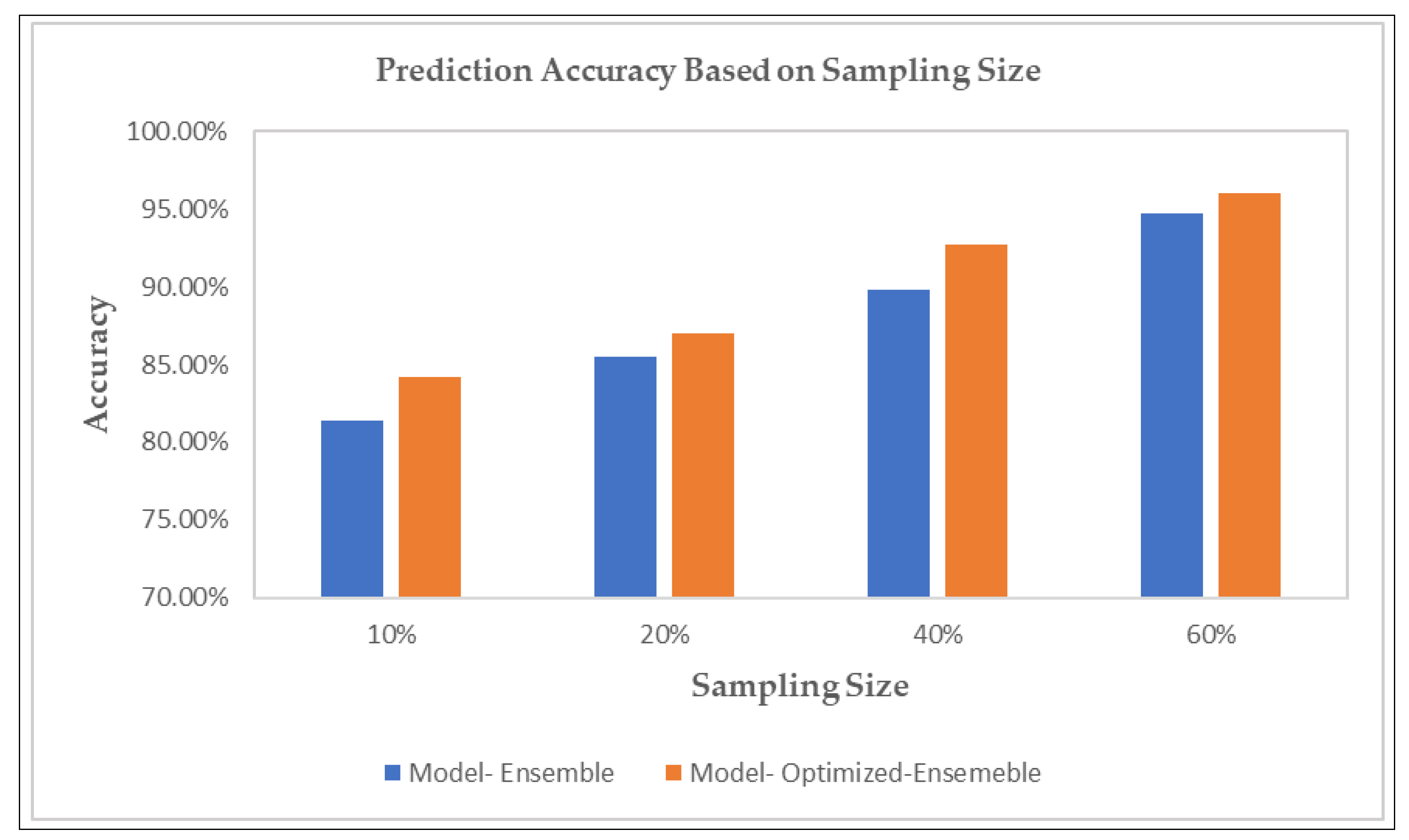
5. Performance Evaluation

In this section, we compare the performance of our proposed model with existing models. In Table 5, we consider individual models, optimized individual models, and ensemble and optimized-ensemble models to evaluate them based on root mean square error (RMSE), mean absolute error (MAE), and mean squared error (MSE). We have taken different combinations of models for the ensemble approach. We have experimented with models such as CatBoost, XGBoost, LightBoost, Random Forest, and Gradient Boosting.

Table 5. Evaluation results based on RMSE, MAE, and MSE for a different combination of models.

Techniques	Models	RMSE	MAE	MSE
Individual	CatBoost	27.89	25.76	789.34
	XGBoost	25.62	23.44	651.88
	LightBoost	26.33	24.90	883.92
	Random Forest	24.54	20.76	671.58
	Gradient Boosting	24.88	22.38	641.46
Optimized-Individuals	CatBoost	27.01	25.12	700.67
	XGBoost	24.94	23.40	619.81
	LightBoost	25.68	22.39	804.48
	Random Forest	23.47	18.91	632.45
	Gradient Boosting	24.61	20.15	621.91
Ensemble	CatBoost, XGBoost, GradientBoost	18.42	17.11	342.76
	CatBoost, LightBoost	20.96	18.78	480.61
	RandomForest, CatBoost	21.55	19.62	520.77
	RandomForest, XGBoost, CatBoost	16.81	15.28	389.51
	CatBoost, XGBoost, LightBoost	11.73	10.53	291.27
Optimized-Ensemble	CatBoost, XGBoost, GradientBoost	17.85	16.22	300.33
	CatBoost, LightBoost	17.99	16.01	451.35
	RandomForest, CatBoost	16.81	18.73	489.36
	RandomForest, XGBoost, CatBoost	10.68	11.83	310.84
	Proposed Model	6.05	5.76	161.37

It can be observed that the best results were achieved when we used optimized-ensemble learning for predictions. Ensemble learning has performed better as compared with the performance of individual models. With individual models, the RMSE range was 24–27, while ensemble models were reduced to the range of 11–22. A similar pattern can be observed for optimized ensembles and optimized individual models.

RMSE measures the deviation in data points or prediction values from the regression line of best fit or the original values. RMSE can be formulated as

$$\mathrm{RMSE}=\sqrt{n{\displaystyle \sum }_{i=1}^n{\left({\sigma }_i-P_i\right)}^2}$$

where P is the prediction and σ is the observed or known values.

MAE calculates the absolute average of all the errors. It refers to the average of absolute values of each prediction error in the test data set considering every instance. MAE is measured as

$$\mathrm{MAE}=\frac{1}{n}{\displaystyle \sum }_{i=1}^n\left|{\sigma }_i-P_i\right|$$

MSE sums the squared residuals and measures the average deviation of the predicted values from the observed values and can be formulated as

$$\mathrm{MSE}=\frac{1}{n}{\displaystyle \sum }_{i=1}^n{\left({\sigma }_i-P_i\right)}^2$$

In Table 6, we have presented the performance comparison of existing models with our proposed model. We have evaluated the current and proposed model on two datasets. Apart from our dataset, we also experimented with publicly available datasets to measure our proposed model’s credibility [48]. We have considered both PSO and GA-based models for comparison. As Table 5 and Table 6 depict, our proposed model generated less error and better performance than existing models on both datasets. The proposed model also outperformed our previously proposed model ANN-PSO [7].

Table 6. Performance comparison with existing models.

Models	Dataset	RMSE	MAE	MSE
PSO-DLNN [49]	Smart meter	18.73	20.86	650.74
	Our Dataset	17.52	20.01	655.33
PSO-XGBoost [50]	Smart meter	17.91	21.99	620.16
	Our Dataset	18.66	19.71	590.42
LDA–GA–SVM [51]	Smart meter	19.23	19.55	590.18
	Our Dataset	15.48	20.79	660.63
ANN-PSO [7]	Smart meter	9.23	11.79	367.49
	Our Dataset	7.82	12.35	401.77
Proposed Model	Smart meter	7.01	9.28	198.36
	Our Dataset	6.05	5.76	161.37

Figure 5 also presents the graphical representation of our prediction model. Yellow depicts the actual energy consumption and green signifies the predicted energy consumption values. We have displayed the results for two months for proper visualization.

Figure 5. Energy consumption prediction.

Prediction accuracy based on a different batch of random sampling sizes is presented in Figure 5. As we can see from Figure 6, prediction accuracy is highest for a sampling size of 60%. We have demonstrated the prediction accuracy for our proposed ensemble model with and without optimization.

Figure 6. Prediction accuracy of the proposed model with and without optimization based on sampling size.

In Figure 7, we have plotted the precision or how close the predictions are to the observed values for existing and our proposed model. As we can see, the precision for our proposed model is the highest, achieving better accuracy.

Figure 7. The precision of the existing and proposed model based on sampling size.

6. Discussion and Concluding Remarks

This paper presents a PSO-centered optimized-ensemble learning and feature selection-based strategy for the energy consumption prediction of smart homes to enhance the prediction outcome. The novelty of this study is in the proposed method based on random sampling and a two-way use of PSO in feature selection and ensemble learning. It enables each prediction model to analyze a different subset of data and generate comparatively highly accurate predictions than an individual model to fit all. Besides that, with inadequate data sizes, the suggested approach is capable of achieving higher prediction outcomes.

The key contributions of this study can be concisely discussed in three parts. Firstly, random sampling was performed on preprocessed data to enhance data quality. Different subsets of data were trained on other models. The purpose of doing this was to figure out an optimal sample size for training. We experimented with various randomly selected data subsets, and it did impact the prediction results with comparatively higher accuracy and lower prediction error. Secondly, according to PSO-based feature importance analysis and selection, the impacts of the energy consumption forecast features were compared. Then the selected features list was optimized, which provided help for the ensemble prediction model. Thirdly, the model of energy consumption prediction was established based on the optimized-ensemble learning. Experiments were performed to evaluate ensemble model performance both with and without PSO optimization of hyper-parameters. Results showed that the idea of using PSO for optimizing the ensemble model enhanced the performance. The reliability of analysis results was verified by testing the model on different publicly available datasets. Finally, the ensemble learning model consisting of five other models, i.e., XGBoost, LightBoost, CatBoost, RandomForest, and Gradient Boosting, was established for each data subset. We experimented with different combinations of the models mentioned earlier to find which hybrid model works best for given data. To evaluate the overall performance of the proposed model, we devised four different techniques where we compared our proposed optimized-ensemble model with the other three techniques. The first technique experiments individual models without any hybrid or combination and PSO optimization. The second technique experiments with PSO optimized individual models. The third technique considers different hybrids, such as a hybrid of CatBoost, XGBoost, GradientBoost, etc. The fourth technique experiments with our proposed optimized-ensemble model. The results are analyzed and compared based on RMSE, MAE, and MSE values. Results showed that compared with other techniques, the proposed method achieved the best prediction effects in each case.

Although our proposed optimized-ensemble learning algorithm has satisfactory energy prediction effectiveness, there is still much room for improvement. We plan to implement and experiment with other sampling techniques in our future work to see if there can be any improvement in the prediction result. The energy consumption patterns of different buildings and households might differ depending upon the individual needs; therefore, the prediction results are also dependent on the underlying usage patterns. Hence, with different circumstances and different usage patterns of various buildings, the proposed model might face some limitations at run time. However, it can incorporate additional features. When the research subject changes or a new running pattern appears, it cannot be updated in time. Therefore, we aim to concentrate on pattern classification of energy usage for different commercial or residential buildings under various environmental and climatic conditions in the future. We aim to recognize and classify new patterns with time automatically.

References

1. Available online: https://www.sciencedirect.com/science/article/pii/B9780128184837000020 (accessed on 22 July 2021).
2. Available online: https://www.irena.org/-/media/Files/IRENA/Agency/Publication/2018/Apr/IRENA_Report_GET_2018.pdf (accessed on 22 July 2021).
3. Available online: https://www.energy.gov/sites/prod/files/2017/01/f34/Electricity%20End%20Uses,%20Energy%20Efficiency,%20and%20Distributed%20Energy%20Resources.pdf (accessed on 22 July 2021).
4. Available online: https://www.iea.org/reports/energy-efficiency-2020/buildings (accessed on 22 July 2021).
5. Jain, R.K.; Smith, K.M.; Culligan, P.J.; Taylor, J.E. Forecasting energy consumption of multi-family residential buildings using support vector regression: Investigating the impact of temporal and spatial monitoring granularity on performance accuracy. Appl. Energy 2014, 123, 168–178. [Google Scholar] [CrossRef]
6. Howard, B.; Parshall, L.; Thompson, J.; Hammer, S.; Dickinson, J.; Modi, V. Spatial distribution of urban building energy consumption by end use. Energy Build. 2012, 45, 141–151. [Google Scholar] [CrossRef]
7. Malik, S.; Shafqat, W.; Lee, K.T.; Kim, D.H. A Feature Selection-Based Predictive-Learning Framework for Optimal Actuator Control in Smart Homes. Actuators 2021, 10, 84. [Google Scholar] [CrossRef]
8. Yu, L.; Wang, Z.; Tang, L. A decomposition–ensemble model with data-characteristic-driven reconstruction for crude oil price forecasting. Appl. Energy 2015, 156, 251–267. [Google Scholar] [CrossRef]
9. Ciulla, G.; D’Amico, A. Building energy performance forecasting: A multiple linear regression approach. Appl. Energy 2019, 253, 113500. [Google Scholar] [CrossRef]
10. Lü, X.; Lu, T.; Kibert, C.J.; Viljanen, M. Modeling and forecasting energy consumption for heterogeneous buildings using a physical–statistical approach. Appl. Energy 2015, 144, 261–275. [Google Scholar] [CrossRef]
11. Arora, S.; Taylor, J.W. Short-term forecasting of anomalous load using rule-based triple seasonal methods. IEEE Trans. Power Syst. 2013, 28, 3235–3242. [Google Scholar] [CrossRef] [Green Version]
12. Kavaklioglu, K. Modeling and prediction of Turkey’s electricity consumption using Support Vector Regression. Appl. Energy 2011, 88, 368–375. [Google Scholar] [CrossRef]
13. Rodrigues, F.; Cardeira, C.; Calado, J.M.F. The daily and hourly energy consumption and load forecasting using artificial neural network method: A case study using a set of 93 households in Portugal. Energy Procedia 2014, 62, 220–229. [Google Scholar] [CrossRef] [Green Version]
14. Tso, G.K.; Yau, K.K. Predicting electricity energy consumption: A comparison of regression analysis, decision tree and neural networks. Energy 2007, 32, 1761–1768. [Google Scholar] [CrossRef]
15. Bouktif, S.; Fiaz, A.; Ouni, A.; Serhani, M.A. Multi-sequence LSTM-RNN deep learning and metaheuristics for electric load forecasting. Energies 2020, 13, 391. [Google Scholar] [CrossRef] [Green Version]
16. Lago, J.; De Ridder, F.; De Schutter, B. Forecasting spot electricity prices: Deep learning approaches and empirical comparison of traditional algorithms. Appl. Energy 2018, 221, 386–405. [Google Scholar] [CrossRef]
17. Salgado, R.M.; Lemes, R.R. A hybrid approach to the load forecasting based on decision trees. J. Control Autom. Electr. Syst. 2013, 24, 854–862. [Google Scholar] [CrossRef]
18. Li, Q.; Ren, P.; Meng, Q. Prediction model of annual energy consumption of residential buildings. In Proceedings of the 2010 International Conference on Advances in Energy Engineering, Beijing, China, 19–20 June 2010; pp. 223–226. [Google Scholar]
19. Ahmad, A.S.; Hassan, M.Y.; Abdullah, M.P.; Rahman, H.A.; Hussin, F.; Abdullah, H.; Saidur, R. A review on applications of ANN and SVM for building electrical energy consumption forecasting. Renew. Sustain. Energy Rev. 2014, 33, 102–109. [Google Scholar] [CrossRef]
20. Gezer, G.; Tuna, G.; Kogias, D.; Gulez, K.; Gungor, V.C. PI-controlled ANN-based energy consumption forecasting for Smart Grids. In Proceedings of the 2015 12th International Conference on Informatics in Control, Automation and Robotics (ICINCO), Colmar, France, 21–23 July 2015; Volume 1, pp. 110–116. [Google Scholar]
21. Bi, Y.; Xue, B.; Zhang, M. An automated ensemble learning framework using genetic programming for image classification. In Proceedings of the Genetic and Evolutionary Computation Conference, Prague, Czech Republic, 13–17 July 2019; pp. 365–373. [Google Scholar]
22. Panthong, R.; Srivihok, A. Wrapper feature subset selection for dimension reduction based on ensemble learning algorithm. Procedia Comput. Sci. 2015, 72, 162–169. [Google Scholar] [CrossRef] [Green Version]
23. Yang, X.; Lo, D.; Xia, X.; Sun, J. TLEL: A two-layer ensemble learning approach for just-in-time defect prediction. Inf. Softw. Technol. 2017, 87, 206–220. [Google Scholar] [CrossRef]
24. Huang, Y.; Yuan, Y.; Chen, H.; Wang, J.; Guo, Y.; Ahmad, T. A novel energy demand prediction strategy for residential buildings based on ensemble learning. Energy Procedia 2019, 158, 3411–3416. [Google Scholar] [CrossRef]
25. Yang, Y.; Hong, W.; Li, S. Deep ensemble learning based probabilistic load forecasting in smart grids. Energy 2019, 189, 116324. [Google Scholar] [CrossRef]
26. Krisshna, N.A.; Deepak, V.K.; Manikantan, K.; Ramachandran, S. Face recognition using transform domain feature extraction and PSO-based feature selection. Appl. Soft Comput. 2014, 22, 141–161. [Google Scholar] [CrossRef]
27. Kumar, S.U.; Inbarani, H.H. PSO-based feature selection and neighborhood rough set-based classification for BCI multiclass motor imagery task. Neural Comput. Appl. 2017, 28, 3239–3258. [Google Scholar] [CrossRef]
28. Tama, B.A.; Rhee, K.H. A combination of PSO-based feature selection and tree-based classifiers ensemble for intrusion detection systems. In Proceedings of the Advances in Computer Science and Ubiquitous Computing, Cebu, Philippines, 15–17 December 2015; Springer: Singapore, 2015; pp. 489–495. [Google Scholar]
29. Amoozegar, M.; Minaei-Bidgoli, B. Optimizing multi-objective PSO based feature selection method using a feature elitism mechanism. Expert Syst. Appl. 2018, 113, 499–514. [Google Scholar] [CrossRef]
30. Rostami, M.; Forouzandeh, S.; Berahmand, K.; Soltani, M. Integration of multi-objective PSO based feature selection and node centrality for medical datasets. Genomics 2020, 112, 4370–4384. [Google Scholar] [CrossRef]
31. Bergstra, J.; Bengio, Y. Random search for hyper-parameter optimization. J. Mach. Learn. Res. 2012, 13, 281–305. [Google Scholar]
32. Available online: https://analyticsindiamag.com/why-is-random-search-better-than-grid-search-for-machine-learning/ (accessed on 16 July 2021).
33. Hutter, F.; Hoos, H.H.; Leyton-Brown, K. Sequential Model-Based Optimization for General Algorithm Configuration. In Learning and Intelligent Optimization; Springer: Cham, Switzerland, 2011; pp. 507–523. [Google Scholar]
34. Snoek, J.; Rippel, O.; Swersky, K.; Kiros, R.; Satish, N.; Sundaram, N.; Patwary, M.M.A.; Prabhat, M.; Adams, R.P. Scalable Bayesian Optimization Using Deep Neural Networks. In Proceedings of the 32nd International Conference on Machine Learning, Lille, France, 6–11 July 2015. [Google Scholar]
35. Lorenzo, P.R.; Nalepa, J.; Kawulok, M.; Ramos, L.S.; Pastor, J.R. Particle swarm optimization for hyper-parameter selection in deep neural networks. In Proceedings of the Genetic and Evolutionary Computation Conference, Berlin, Germany, 15–19 July 2017; pp. 481–488. [Google Scholar]
36. Lorenzo, P.R.; Nalepa, J.; Ramos, L.S.; Pastor, J.R. Hyper-parameter selection in deep neural networks using parallel particle swarm optimization. In Proceedings of the Genetic and Evolutionary Computation Conference Companion, Berlin, Germany, 15–19 July 2017; pp. 1864–1871. [Google Scholar]
37. Wang, Y.; Zhang, H.; Zhang, G. cPSO-CNN: An efficient PSO-based algorithm for fine-tuning hyper-parameters of convolutional neural networks. Swarm Evol. Comput. 2019, 49, 114–123. [Google Scholar] [CrossRef]
38. Nalepa, J.; Lorenzo, P.R. Convergence analysis of PSO for hyper-parameter selection in deep neural networks. In Proceedings of the International Conference on P2P, Parallel, Grid, Cloud and Internet Computing, Yonago, Japan, 28–30 October 2017; Springer: Cham, Switzerland, 2017; pp. 284–295. [Google Scholar]
39. Guo, Y.; Li, J.Y.; Zhan, Z.H. Efficient hyperparameter optimization for convolution neural networks in deep learning: A distributed particle swarm optimization approach. Cybern. Syst. 2020, 52, 36–57. [Google Scholar] [CrossRef]
40. Palaniswamy, S.K.; Venkatesan, R. Hyperparameters tuning of ensemble model for software effort estimation. J. Ambient Intell. Hum. Comput. 2021, 12, 6579–6589. [Google Scholar] [CrossRef]
41. Tan, T.Y.; Zhang, L.; Lim, C.P.; Fielding, B.; Yu, Y.; Anderson, E. Evolving ensemble models for image segmentation using enhanced particle swarm optimization. IEEE Access 2019, 7, 34004–34019. [Google Scholar] [CrossRef]
42. Khanesar, M.A.; Teshnehlab, M.; Shoorehdeli, M.A. A novel binary particle swarm optimization. In Proceedings of the 2007 Mediterranean Conference on Control & Automation, Athens, Greece, 27–29 June 2007; pp. 1–6. [Google Scholar]
43. Malik, S.; Kim, D. Prediction-learning algorithm for efficient energy consumption in smart buildings based on particle regeneration and velocity boost in particle swarm optimization neural networks. Energies 2018, 11, 1289. [Google Scholar] [CrossRef] [Green Version]
44. Cui, G.; Qin, L.; Liu, S.; Wang, Y.; Zhang, X.; Cao, X. Modified PSO algorithm for solving planar graph coloring problem. Prog. Nat. Sci. 2008, 18, 353–357. [Google Scholar] [CrossRef]
45. Chau, K.W. Particle swarm optimization training algorithm for ANNs in stage prediction of Shing Mun River. J. Hydrol. 2006, 329, 363–367. [Google Scholar] [CrossRef] [Green Version]
46. Feurer, M.; Klein, A.; Eggensperger, K.; Springenberg, J.; Hutter, F. Efficient and robust automated machine learning. In Proceedings of the Advances in Neural Information Processing Systems 28 (NIPS 2015), Montreal, QC, Canada, 7–12 December 2015. [Google Scholar]
47. Jiang, M.; Jiang, S.; Zhi, L.; Wang, Y.; Zhang, H. Study on parameter optimization for support vector regression in solving the inverse ECG problem. Comput. Math. Methods Med. 2013, 2, 158056. [Google Scholar] [CrossRef] [PubMed] [Green Version]
48. Available online: https://www.kaggle.com/taranvee/smart-home-dataset-with-weather-information (accessed on 5 July 2021).
49. Band, S.S.; Janizadeh, S.; Pal, S.C.; Saha, A.; Chakrabortty, R.; Shokri, M.; Mosavi, A. Novel ensemble approach of deep learning neural network (DLNN) model and particle swarm optimization (PSO) algorithm for prediction of gully erosion susceptibility. Sensors 2020, 20, 5609. [Google Scholar] [CrossRef] [PubMed]
50. Qin, C.; Zhang, Y.; Bao, F.; Zhang, C.; Liu, P.; Liu, P. XGBoost Optimized by Adaptive Particle Swarm Optimization for Credit Scoring. Math. Prob. Eng. 2021, 2021, 1–18. [Google Scholar]
51. Ali, L.; Wajahat, I.; Golilarz, N.A.; Keshtkar, F.; Chan Bukhari, S.A. LDA–GA–SVM: Improved hepatocellular carcinoma prediction through dimensionality reduction and genetically optimized support vector machine. Neural Comput. Appl. 2021, 33, 2783–2792. [Google Scholar] [CrossRef]
Publisher’s Note: MDPI stays neutral with regard to jurisdictional claims in published maps and institutional affiliations.
Article Metrics
Citations
Article Access Statistics
Multiple requests from the same IP address are counted as one view.