Abstract
A new configuration of a pseudo-correlation type radiometer is proposed for a microwave biomedical application, such as diabetic foot neuropathy. The new approach as well as its simulated performance are thoroughly assessed using commercial off-the-shelf components and custom designed subsystems. We configured a pseudo-correlation receiver, centred at 3.5 GHz, to validate the proposal, comparing its simulated response with a measured alternative based on a 90 hybrid coupler pseudo-correlation prototype. We custom designed a balanced Wilkinson power divider and a 180 hybrid coupler to fulfil the receiver’s requirements. The proposed configuration demonstrated an improved noise temperature response. The main advantage is to enable the recalibration of the receiver through simultaneous measurable output signals, proportional to each input signal, as well as the correlated response between them.
1. Introduction
Microwave Radiometry (MWR) is the measurement technique involved in the characterization of the natural electromagnetic radiation in the microwave spectrum. This technique has been commonly employed in many areas, encompassing physics, chemistry, and engineering [1]. In connection with the radio astronomy field, its typical receiver configurations have been applied to biomedical applications for the detection and diagnosis of pathologies in which an internal temperature gradient has been observed [2,3]. As a non-ionizing, non-invasive and inherently safe technique, MWR enables the measurement of internal body temperatures with or without contact for the early diagnosis of several pathologies [3,4,5].
Microwave technology has confirmed its effectiveness to provide temperature patterns at a depth of several centimetres [6,7]. The internal temperature of human body tissues can differ several degrees from that of the surface or skin [8]. Thus, monitoring both internal as well as superficial temperatures and analysing their differences constitutes a significant issue for a variety of medical diagnostic and treatment procedures [9]. In this regard, several medical applications have already implemented MWR systems for the detection of superficial breast cancer, atherosclerosis, rheumatoid arthritis, diabetic pathologies, urogenital diseases, as well as the measurement of internal brain temperatures [2,3,5,10,11,12,13,14,15,16,17,18]. MWR has been also demonstrated in preclinical research for the analysis of the thermal radiation of internal tissues, assessing temperature changes in malignant tumours that may serve as a diagnostic marker [19].
X-rays, ultrasound, and magnetic resonance imaging (MRI) are widespread techniques used in clinical applications. However, these techniques show some disadvantages or limitations, such as cost, sensitivity or discomfort depending on the application [10]. MRI and X-rays are generally expensive and non-portable, but show high spatial resolution [20]. In addition, X-rays are considered as ionizing radiation. On the other hand, internal thermometers are also employed to measure temperatures within the body, but they are invasive, not convenient for long-term monitoring and cause discomfort to patients [21]. Thus, the main goal of MWR is to provide a non-ionizing, non-invasive, fast, low-priced, and passive system that is able to penetrate into the tissues.
Microwave frequencies improve transmission features in comparison with infrared thermography when applied to human body tissues [22]. The infrared transmission depth within tissues is truly small, and the detected radiation essentially comes from the surface of the skin [22]. MWR is directed at detecting the thermal radiation originating from the internal layers or tissues, minimizing the effect of the skin. The penetration depth of microwave radiation depends on the dielectric properties and water content of the targeted tissues; however, lowering the frequency has demonstrated greater detection depths [2,23]. Human body tissues behave as partially transparent layers for the electromagnetic radiation at microwave frequencies, particularly below 6 GHz. Thus, microwave thermal radiation can be detected up to a few centimetres since penetration depth is in the same order of the radiation wavelength [6].
However, a significant difference is still noticed between the radiated energy at the infrared and microwave ranges. The radiation intensity at microwave frequencies is considerably lower than the one at the infrared spectrum, and close to detection limits [5]. Therefore, a very sensitive receiver is required to detect the tiny power levels naturally radiated from biological tissues.
MWR systems proposed for medical applications have been commonly implemented following a Dicke topology, using a switch at the input [9,24,25,26,27,28,29,30,31,32]. The incoming signal is, therefore, periodically switched with a known reference, providing a differential output of the detected signals in correspondence to each input. These systems usually provide long-term continuous measurements in which gain and noise fluctuations are removed by selecting an appropriate switching frequency.
Alternative solutions for biomedical applications based on pseudo-correlation topologies can be implemented [33]. This configuration is typically employed on astrophysical instrumentation [34,35,36] and presents an improved performance. The system offers a simultaneous observation of two signals with a smaller dependence on gain fluctuations [37], a longer observation time, as well as higher stability. The receiver should be calibrated to convert the input power to temperature and remove gain fluctuations to provide a continuous output signal during a long-term period of time.
Significant differences are found between astrophysical and medical applications. A narrow input dynamic range is required to measure body temperatures at short distances [26], opposite to the large bandwidths and huge distances relevant in astrophysical applications. MWR systems can be designed using commercial off-the-shelf (COTS) components that reduce the size of the receiver. In addition, long and continuous observation times are employed on astrophysical instrumentation to improve the minimum detectable temperature or sensitivity, enabling the detection of faint radio sources [1]. Thus, the receiver requires periodical calibrations to overcome and correct fluctuations on the receiver noise temperature and gain.
Although this effect is also important and calibration is required for MWR receivers aimed at biomedical applications, instantaneous measurements should be performed to avoid patient discomfort due to extended examination times. For these reasons, a new receiver configuration is required to provide a reduced contribution to the total noise temperature as well as additional output signals to calculate drift effects and recalibrate its response.
In this context, the final goal is to define a clinical workflow for diabetic foot neuropathies in which superficial and internal temperature measurements are combined. Initially, an infrared sensor acquires images from the skin surface [38,39,40], providing the superficial temperature. Subsequently, after image processing, anomalous temperature patterns are detected over specific areas, in which MWR is employed to provide complementary in-depth measurements for further analysis [33]. Thus, a MWR system able to detect significantly small radiated power differences from tissues is required, while adding the lowest achievable noise contribution.
The measured temperature is derived from the system calibration, which requires the extraction of the receiver response curve and the correction of any drift on its performance. The proposed system is dedicated to providing clinical practitioners a diagnostic tool to improve their capabilities, which, in combination to already established technologies, may provide significant advances in monitoring the targeted pathologies. In this particular case, the proof-of-concept technology provides a diagnostic tool intended for diabetic foot neuropathies [16,41], although other soft tissue pathologies, in which diagnosis, detection, and monitoring based on temperature measurements, can be targeted.
The diagnosis of lung complications derived from COVID-19 disease is also supported by internal measurements yielded by a MWR system [42]. The microwave system supplies internal temperature measurements of body tissues, which complements the superficial measurement given by infrared sensors [43]. MWR has already demonstrated a significant detection improvement when applied to diabetic patients, with satisfactory sensitivity and specificity rates [16], and new approaches are being modelled to early detect foot ulcers [41]. Thus, potential risks can be detected prior to a visible sign on the skin surface or irreversible damage is caused.
This paper is focused on the design of a new receiver configuration based on a pseudo-correlation type radiometer for a medical application, particularly diabetic foot neuropathies. The aim of the proposed balanced topology is to provide measurable detected signals to correct drifts in its performance, and to simultaneously reduce the noise introduced by the receiver. Thus, the main advantage is the possibility to obtain an unknown input temperature after the initial calibration is performed, employing the set of signals provided by the receiver, adjusting the calibration and correcting its drifts during the measurement. The output signals are proportional to the input ones and, simultaneously, to the combination between them, using 180 hybrid couplers together with power splitters.
Then, the analysis of this set of signals provides additional information to extract the noise contributions of each component in the receiver chain and possible fluctuations in the output signals that can be subsequently corrected. The receiver is designed using commercial COTS measured microwave devices and custom designs with electromagnetic simulations of hybrid couplers and power splitters. The proposed receiver is centred at 3.5 GHz for comparison to a previously implemented pseudo-correlation radiometer [33]. Additionally, at this frequency, a reasonable compromise is achieved between the spatial resolution and depth measurements in lossy tissues, as well as less electromagnetic interferences than at lower frequencies [28].
2. Background Overview of MWR Systems for Medical Applications
MWR systems are intended to detect very small temperature variations in subcutaneous layers. Thus, the radiometer should be configured to provide high sensitivity, low noise, and low gain drift for a continuous measurement [9]. In addition, the operation frequency of the receiver should be low enough to provide a penetration depth of several centimetres into tissues [6].
The Dicke topology has been typically employed in MWR systems for biomedical applications [9,24,25,26,27,28,29]. They have been designed using COTS components, centred at diverse frequency bands and focused on monitoring internal body temperatures of a single tissue or a stack of tissue layers. Figure 1 illustrates the commonly implemented configuration, in which a switch located at the antenna output alternates the incoming signal with a single- [28] or two-reference load [9,26].
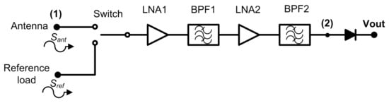
Figure 1.
A typical radiometer configuration for medical applications using a switched Dicke topology.
Thus, a two-level half-cycle output signal of the sequential input measurements is provided at the output port of the receiver. This topology is able to remove gain fluctuations by appropriately selecting the switching frequency [34]. Then, the receiver is calibrated at the sample rate defined by the switching signal, since the receiver periodically measures a known input signal and corrects the drifts in its response. The amplification stage should be designed considering the detectable power window at the detection stage, as well as the low noise power level radiated from body tissues. The noise power radiated from an object in the microwave spectrum is approximated by Rayleigh-Jean’s law and expressed as
where k is the Boltzmann constant, T (K) is the temperature, and B (Hz) is the effective bandwidth. Then, an equivalent power of around −174 dBm/Hz is radiated from body tissues at a temperature of 310 K (37 C).
The analysis of the Dicke receiver shown in Figure 1 provides two alternating half-cycle detected output signals, expressed as
and
where C is a proportionality constant, G is the gain of the receiver, k is the Boltzmann constant, B is the effective bandwidth, Tant is the noise temperature measured by the antenna, Tref is the noise temperature of the reference load, and Trec is the equivalent noise temperature of the receiver, which is calculated as
where TLNA1 and TLNA2 are the equivalent noise temperatures of LNA1 and LNA2 with gains GLNA1 and GLNA2 respectively. LSW, LBPF1, and LBPF2 are the losses of the switch, BPF1, and BPF2, respectively, all at a physical temperature Tph, equivalent to the ambient temperature.
Dicke radiometers cancel gain fluctuations in the system for a sufficiently high modulating frequency [34], despite the radiometric sensitivity being degraded since the target is only measured half of the time [44].
A Dicke configuration is not unique for biomedical applications. Other commonly used schemes implemented in astrophysical instrumentation, such as correlation or pseudo-correlation topologies [34,35], can be applied [33]. The main advantage of correlation schemes is to avoid the input switch to alternate between signals. A correlation radiometer multiplies different input signals coming from antennas employing identical receivers connected in parallel and providing a single correlated output [45]. The pseudo-correlation radiometer combines the comparison with a reference load from the Dicke radiometer with the combination of signals from the correlation radiometer but providing additional output signals [36].
Using the latter topology, a simultaneous observation of two voltage signals, antenna and reference load inputs, are available during the measurement process, providing a continuous output voltage proportional to the difference between the two input signals [33]. In addition, a higher stability, voltage sensitivity, and observation time are improved in comparison to the Dicke scheme [36,37,46]. Finally, correlation techniques reduce the impact of intrinsic gain and noise temperature fluctuations in comparison to conventional configurations [47]. Table 1 lists some microwave radiometers employed for biomedical applications for comparison purposes. Simulation results based on real measurements are compared with other MWR systems, and a significant noise temperature reduction is observed with the proposed new configuration.

Table 1.
Comparison between the proposed radiometer and other MWR systems for biomedical applications.
From a simplified analysis of the scheme proposed in [33], which considers a perfect isolation between hybrid coupler ports and avoids mismatching effects, two in-phase voltage signals are provided at output ports prior to combining them. These are proportional to the individual incoming signals at the reference load and the antenna ports, respectively [33].
For the calculation of the equivalent noise temperature of the pseudo-correlation receiver, Trec2, identical subsystems are considered in both branches, which means that, for example, the noise of the amplifiers are equal in magnitude, although they are not correlated [48]. Thus, it is expressed as
-4.6cm0cm
where TLNA1i is the equivalent noise temperatures, GLNA1i is the gains of each LNA1i (with i = 1, 2, 3), and Li is the losses associated with band-pass filters (i = BPF1j, with j = 1, 2, 3) or 90 hybrid couplers (i = H90j, with j = 1, 2), respectively, all of them at a physical temperature Tph, equivalent to the ambient temperature.
3. Microwave Receiver Analysis
3.1. 180 Hybrid Coupler Pseudo-Correlation Configuration
A new receiver topology is proposed for biomedical applications. This configuration is based on a pseudo-correlation scheme using 180 hybrid couplers, with added power splitters, prior to the second hybrid coupler stage. Figure 2 shows the proposed schematic. This proposal enables the receiver to provide a sample of both output signals proportional to the input ones and, at the same time, their combination.
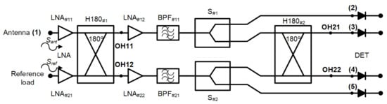
Figure 2.
The new pseudo-correlation schematic using 180 hybrid couplers to correlate the signals and Wilkinson power dividers.
Analysing the receiver configuration, the output voltages of the first hybrid coupler, H180#1 in Figure 2, are defined as
These outputs are equally split into two using Wilkinson power dividers. Then, one of the outputs of each power divider is directly detected, whereas the other one corresponds to an input signal of the second 180 hybrid coupler. This coupler correlates the split SOH11 and SOH12 signals, providing output voltage signals proportional to the input ones Sant and Sref. The output signals of the second hybrid are expressed as
Both signals SOH21 and SOH22 are detected using square-law microwave diode detectors and, simultaneously, the combinations of the input voltage signals are also provided and detected.
3.2. Noise Analysis
This section describes the equivalent noise temperature of the proposed receiver. The equivalent noise temperature when the system is under operation, Top, is defined as
where Tant is the noise temperature measured by the antenna, and Trec3 is the equivalent noise temperature of the receiver. Therefore, as both noise temperatures are additive, a minimum noise temperature contribution of the receiver is desired.
The equivalent noise temperature, Trec3, of the new proposed configuration, considering the same assumptions as for Equation (5), can be calculated as
where TLNA11 and TLNA12 are the equivalent noise temperatures of LNA11 and LNA12, GLNA11 and GLNA12 are the gains of LNA11 and LNA12, Li is the losses associated with the 180 hybrid couplers (i = Hj, with j = 1, 2), band-pass filter (i = BPF11) and power splitters (i = S1), respectively, all of them at a physical temperature Tph, equivalent to the ambient temperature.
This receiver topology provides a lower noise temperature than the Dicke receiver or the pseudo-correlation radiometer based on 90 hybrid couplers [33], since the first element is a low-noise amplifier with low noise temperature and high gain.
3.3. Receiver Analysis
The microwave receiver was analysed to obtain the output expressions at each output port [49]. The voltages Sant and Sref, coming from the antenna and reference load inputs, are the propagation inputs through the system. A simplified schematic of the receiver was employed to perform the analysis, without considering the detection. In addition, the amplification and filtering stage after H180#1 was considered as a single element, including the noise contributions of both LNA and BPF.
The schematic is shown in Figure 3. Each signal initially goes through two low-noise amplifiers LNA#11 and LNA#21, prior to accessign the 180 hybrid coupler H180#1. The voltages are further amplified and filtered before they are divided into two equal parts in S#1 and S#2. Finally, H180#2 provides the combination of the two output voltages coming from the first hybrid coupler.
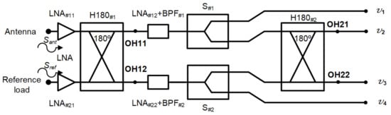
Figure 3.
Simplified schematic of the proposed receiver to perform its analysis.
The output signal of each subsystem in the receiver is obtained using the transfer function of each one that is defined and listed in Table 2. The low-noise amplifiers are considered to show a voltage gain gi > 1, whereas the passive subsystems have a voltage loss ai < 1, and ni the noise added by each subsystem.
Table 2.
The microwave receiver subsystem transfer functions for the proposed configuration, with k = 1 for the upper branch #1, and k = 2 for the lower branch #2 of the schematic in Figure 2.
The analysis considers that every pair of subsystems in each branch (amplifiers, band-pass filters, hybrids couplers, and power splitters) has identical voltage gain or loss and phase. This means that, for example, the amplifiers LNA#11 and LNA#21 show identical gains ga11 = ga21 and phases a11 = a21, but different noise contributions, na11 and na21, for each input LNA.
The output signals are a combination of the input signals, together with the noise added by the receiver subsystems. Therefore, the output voltages at the different ports can be expressed as
where
Subsequently, these signals are detected using square-law detectors, and the corresponding output voltages Vi are expressed as
As can be seen, a negligible contribution to the noise from the hybrid couplers, filters, and power splitters is considered since a high gain value in the low-noise amplifiers is expected. Therefore, the main noise contribution is assumed to be provided by the first amplifier as expected.
Finally, the equivalent electrical temperature at each output port, Teqi, can be calculated as
where Vi represents the output voltage at each port, k is the Boltzmann constant, and B si the effective bandwidth for each output.
Using Equations (12) to (15), the noise temperature at each output port, prior to detection, can be measured. Then, the system can be solved in terms of the output powers at each port to calculate the set of parameters of the receiver. The output powers are expressed as
where GT and Gh represent the power gains from input to power splitter output (equivalent to gT2) and to the second hybrid output (equivalent to gT2·aH22), respectively, and Tant, Tref, and Trec3 are the equivalent noise temperatures of the antenna, the reference load, and receiver, respectively. The detected voltages at each output are proportional to the powers described in Equations (22) to (24), applying the sensitivity value of the microwave detectors, expressed as
where is the voltage sensitivity (V/W) of the detectors.
The receiver noise temperature is obtained applying the Y-factor [50] using two loads with different temperatures, Thot and Tcold, at the receiver input, as
where Y=Phot/Pcold, with Phot and Pcold as the noise powers for both source states at the output of the receiver. As Tref is a known parameter, Gh can be calculated using Equation (23) as
Subsequently, Tant is calculated as
Lastly, once these parameters are obtained, GT can be calculated as
As the initial step to demonstrate Equations (22) to (24), an ideal noiseless simplified receiver, including ideal hybrid couplers and power splitters, is simulated to validate the noise analysis, without any amplification or filtering included. The simulated results in terms of noise temperatures are listed in Table 3, when three sets of input signals are applied to the receiver: Tant = 400 K and Tref = 100 K; Tant = 500 K and Tref = 250 K; and Tant = 310 K and Tref = 290 K.
Table 3.
Simulated temperatures at 3.5 GHz at each predetection point for different input signals for a noiseless receiver (Trec3 = 0 K) and without amplification and filtering stages.
The simulated values demonstrate the described performance in Equations (22) to (24), since the theoretical electrical temperatures obtained in the different predetection points are proportional to the input temperatures considering a completely balanced and noiseless receiver, as listed in the last column of Table 3.
4. Receiver Design and Results
4.1. System Design
The proposed receiver is partially designed using COTS components. They are listed in Table 4, in which their typical performances are summarized as provided by the manufacturer [51,52], and shown in Figure 4. However, some of the involved subsystems are custom designed to fulfill the requirements of the receiver.
Table 4.
COTS components employed in the receiver design.
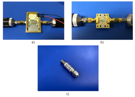
Figure 4.
Photographs of the COTS components: (a) Low-noise amplifier TAMP-362GLN+ (case style JQ1382) assembled on its evaluation board. (b) Band-pass filter BFCN-3600+ (case style FV1206) assembled on its evaluation board. (c) Schottky diode coaxial detector ACSP-2643NZC3.
The input power at the antenna port is estimated to be around −174 dBm/Hz for tissues at 310 K (37 C). Thus, each branch is composed of three-stage low-noise amplifiers to achieve the detectable window of microwave detectors. The first pair of LNAs are located prior to the first hybrid, just after the antenna and reference load inputs. After the hybrid coupler, a cascaded two-stage set composed of LNA+BPF are placed to provide further amplification and confining of the band. At this point, both signals are equally split using the power dividers. Finally, two samples of these signals are correlated again.
The custom designed subsystems correspond to the hybrid couplers and the power dividers. The 180 hybrid coupler is configured using a rat-race topology, whereas the power divider follows a two-way Wilkinson topology [53]. Further design details are explained in the next section.
4.2. Performance Results
This section shows the simulation results of the designed subsystems for the receiver, as well as its whole performance.
The 180 hybrid coupler, designed in a rat-race topology on a CLTE-XT substrate (a 0.254-mm thickness, r = 2.94, and 0.017-mm copper layer), is shown in Figure 5. This displays the optimized impedances and lengths of the microstrip lines to achieve an improved overall response in terms of the phase and amplitude balances as well as impedance matching. The CLTE-XT substrate was selected since it provides a reasonable trade-off between matching, coupling factor, losses, size, and ease in the manufacturing process compared with higher dielectric constant substrates.
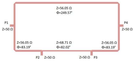
Figure 5.
180 hybrid coupler designed on a CLTE-XT substrate. Size: 31.5 mm × 15.6 mm.
Initially, the theoretical classical configuration was considered for the hybrid coupler [53], and thus the ports were placed at a quarter wavelength away from each other around the first half of the ring, whereas the second half of the ring had three-quarter wavelengths. The impedance of the transmission lines was selected as times the port impedance (50 ). This theoretical configuration provided a narrow band response; therefore, during the optimization process using the momentum from ADS software (Keysight Technologies), both the impedances and the lengths of the transmission lines within the ring were modified to achieve a better performance in a wider frequency band.
The optimization goals were simultaneously defined in the frequency range from 2 to 5 GHz in terms of low deviations in phase (±3) and amplitude (±0.5 dB) balances from the theoretical ones, as well as return loss higher than 15 dB at each port. Figure 6 depicts the results in terms of input matching at each port, transmission of direct and coupled branches from P1 and P3 as input ports, phase and amplitude imbalances, and A, between outputs.
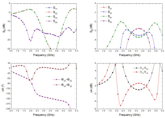
Figure 6.
180 hybrid coupler electromagnetic simulation.
The proposed Wilkinson power divider was designed on the same substrate and is shown in Figure 7. The 100 resistor is not included in the layout; however, the points in which it is placed are indicated. Considering the theoretical configuration of a Wilkinson power divider [53], the 50 input line is split into two quarter wavelength transformers with an impedance of times the port impedance (50 ), and the resistor connects the end point of both transformers as shown in the figure. This configuration simultaneously provides equal split, isolation, and matching.
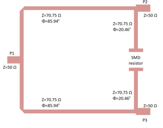
Figure 7.
Wilkinson power divider designed on the CLTE-XT substrate, showing the ports and the location of the 100 SMD resistor (imperial code 0805). Size: 13.5 mm × 10.4 mm.
The lines were slightly optimized using electromagnetic simulations (momentum) to fulfil the requirements in terms of phase and amplitude balances. The final impedances and the lengths of the lines are described in Figure 7. The electromagnetic simulation of the circuit was performed and, then, an electrical model simulation was performed, including the surface-mount-device (SMD) resistor using a model from ADS. The simulation results are depicted in Figure 8, showing input matching at each port, transmission between input and both output ports, as well as the phase and amplitude imbalances, and A respectively, between the transmitted signals from input to outputs.
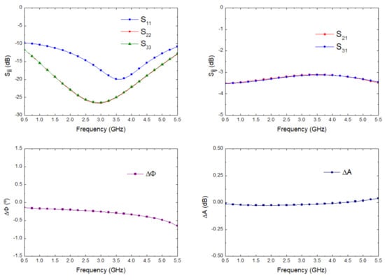
Figure 8.
Wilkinson power divider electromagnetic simulation.
Once these two subsystems were designed and their responses in terms of phase and amplitude balances were verified and validated, the whole proposed receiver was simulated in terms of scattering parameters and noise figure using ADS. Each subsystem in the schematic shown in Figure 2 was replaced with data including their performances. Both LNA and BPF, listed in Table 4, are COTS components, and their measurement results were employed, whereas the presented electromagnetic simulations described above were used for the hybrid couplers and power dividers.
The simulation of the input matching at each port, the transmission from antenna port to each output port correspondingly labelled in the schematic shown in Figure 2, and the noise figure and noise temperature, from antenna input to predetection port labelled as (4), are shown in Figure 9. The receiver noise simulation exhibited an average noise figure of 1.09 dB and noise equivalent temperature of 82.57 K within 2.5 GHz to 4.5 GHz. These values improved the described ones for the 3.5 GHz pseudo-correlation radiometer originally proposed, with 1.39 dB and 109.37 K as the average simulated values and 1.71 dB and 140.26 K as the average measurements within the same band for the noise figure and noise temperature, respectively [33].
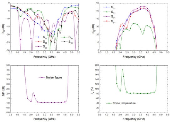
Figure 9.
The simulated scattering parameters from the antenna input to each output port, noise figure, and equivalent noise temperature of the proposed receiver.
The effective bandwidth B of a the radiometer can be expressed as [34,44,46]
where G(f) is the power gain prior to the detection stage. According to the simulated gain of the direct output port corresponding to the antenna input (OH22 in Figure 2 and S41 in Figure 9), an effective bandwidth of 1.26 GHz was calculated.
Subsequently, the receiver, including the scattering and noise performances of the subsystems and, therefore, the simulated noise of the receiver shown in Figure 9, was simulated for Tant = 400 K and Tref = 100 K; and Tant = 310 K and Tref = 290 K. In addition, Table 5 lists the measurable output power at each predetection point when Tant = 310 K and Tref = 290 K were employed as inputs, using the calculated effective bandwidth at each output.
Table 5.
The simulated output power at each predetection point in the schematic of Figure 2 for an input signal at antenna port equivalent to body tissues temperature Tant = 310 K (Tref = 290 K).
Furthermore, the analysis introducing a varying power level broadband noise-like signal at antenna port was also performed. Laboratory noise sources provided an excess noise ratio, ENR, which was modified using attenuators. Thus, a varying ENR was configured in the simulations, with values from 3 to 12 dB in 3 dB steps, to provide the input power of the noise signal TENR, calculated as
where T0 = 290 K and ENR (dB) is the simulated excess noise ratio value. The reference load port was properly matched with a 50 load. The results of the simulated output powers at each predetection point are listed in Table 6.
Table 6.
The simulated output power at each predetection point in the schematic of Figure 2 for varying power level noise-like input signals at the antenna port using a noise source (Tref = 290 K).
4.3. Receiver Calibration Procedure and Application
The described receiver in the previous section was composed of non-ideal components, showing limited isolation or amplitude and phase balances. Therefore, a calibration was required to correct its performance and calculate the output values in an accurate way. The proposed calibration procedure was based on applying a set of noise temperatures at each input port, whereas the other one was loaded with a fixed value. Then, two noise temperatures were applied at both receiver’s inputs, Tant and Tref, to calculate the power conversion considering the limitations of the receiver. At each output, the output powers were calculated and correction coefficients were obtained.
Ideally, the power associated with Tref is delivered to the predetection point labelled as (3) in Figure 2, in which PV2 is measured. However, a small contribution coming from Tant was present due to the isolation limitations of the hybrid couplers. Thus, when calibrating the output associated with this port, two noise temperatures were provided at the reference port, Tref, as well as at the antenna Tant, giving a combination of power levels obtained as
with i = 1, 2 for each input noise temperature at Tanti, and with j = 1, 2 for both noise temperatures at Trefj. The parameters 2 and 2 correspond to the direct and leakage contributions coming from each input port, respectively, and are calculated as
and
Then, the receiver noise temperature Trec3 is calculated using the Y-factor as
where Y=PV2 @ Tref2/PV2 @ Tref1 and Tant1 the fixed value for both temperature values at Trefj. This expression provides a corrected calculation for the equivalent noise temperature of the receiver instead of Equation (26), including the receiver’s limitations.
Similarly, the procedure was also applied to calibrate the predetection point (4) in Figure 2, in which PV3 is measured and ideally proportional to Tant, defined as
and calculating the parameters 3 and 3 as
and
PV1 and PV4 correspond to the output power levels at predetection points (1) and (5) in Figure 2, after being split by the first hybrid coupler. They are calibrated following the same procedure, employing the above calculated parameters, and the output powers are expressed as
and
with i = 1, 2 for each input noise temperature at Tant and j = 1, 2 for both noise temperatures at Tref.
The new set of parameters, 11, 12, 13, 41, 42, and 43, are required to calibrate the receiver. These parameters 11, 12, 13, 41, 42, and 43 are then calculated as
with k = 1, 4 for each output of the receiver corresponding to PV1 and PV4, respectively.
Considering a common parameter, the set of output powers can be expressed as a single equation, given by
with = 2, and Ak, Rk, and Nk are constant values for each parameter as defined in Equations (33), (34), (37), (38), and (42) to (44) normalized to 2 corresponding to each temperature at the antenna access, reference access, and equivalent noise temperature of the receiver, respectively. These normalized values are defined in Table 7.
Table 7.
The calibration parameters calculated for a set of temperatures of 290 and 500 K applied to both inputs normalized to 2 = 4.750 × 10⁻⁹ W/K.
The proposed procedure was applied to the system, with input temperatures of 290 K and 500 K employed at both inputs and swapped between them. Then, the power levels at each predetection point were simulated, and the calibration parameters were calculated and are listed in Table 7 for 2 = 4.750 × 10⁻⁹ W/K. In addition, an equivalent noise temperature of the receiver, Trec3, of 81.73 K was obtained applying Equation (35). This value takes into account the radiometer response integrating its whole gain and noise performances across the band.
Once these calibration parameters are obtained, any temperature at antenna port can be measured. Two reference loads at the reference port enable the correction of the parameter and Trec3 in real-time without requiring a new calibration. These values were applied to calculate Tant, correcting the receiver’s gain and noise temperature drifts. The two reference noise temperatures are provided by a noise source on its ON and OFF states, TrefH and TrefC, respectively. Then, two output power levels are measured for the unknown antenna temperature. The αmed parameter was obtained employing the output powers PV1 and PV4 at predetection points (1) and (5) in Figure 2, from Equation (45) as
whereas the output power at predetection point (2) in Figure 2, PV2, was employed to obtain the value of Trec3med as
where Ymed = PV2 @ TrefH/PV2 @ TrefC. Finally, the measured value of the antenna temperature, Tantmed, was calculated using PV3, the previous measured αmed, and Trec3med, and the calibration parameters as follows
The latter expression takes into account the correction of the leakages in the receiver. The R3 parameter defines the leakage of the added power from Tref to the predetection point (4) in Figure 2 (proportional to β3), while the A2 parameter corrects the leakage from Tant to the predetection point (3) in Figure 2 (proportional to β2).
4.4. Validation of the Measurement Procedure Employing the Foot’s Temperature Patterns
The MWR system is intended to be employed in the analysis of diabetic foot neuropathies, in a combined clinical workflow with thermal infrared sensors [38]. As a proof of concept, the validation of the proposed measurement procedure was performed employing known temperatures obtained from thermal images. Despite the values correspond to superficial temperatures, they can be used as reference values to validate the method since the temperature gradient observed is of the same order of magnitude as that expected for internal temperature measurements.
Then, images of two volunteers were acquired using a Thermal Expert TE-Q1 Plus infrared camera. After image processing to remove the background and segment the foot’s soles [39], the temperature patterns of the right foot for each volunteer were obtained and are shown in Figure 10. Heterogeneous temperature patterns were observed for both volunteers, thus, enabling the receiver to validate its response with different input values. Single dimension arrays of temperatures along the x- and y-axis lines were selected from each pattern as depicted in the figure in the form of a black line. Five temperature points were considered within each foot’s soles, in which a gradient was observed, and these are listed in Table 8 as Treal-1 and Treal-2 for each pattern.
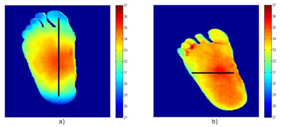
Figure 10.
The temperature patterns of the right foot acquired employing the infrared camera (temperature values in degrees Celsius, equivalent to T (C) = T (K) − 273.15). (a) Volunteer #1. (b) Volunteer #2.
Table 8.
The temperatures obtained from the simulation of the radiometer using the temperatures patterns of the volunteers.
Once the foot’s sole temperatures were known, they were employed as input temperatures for the microwave receiver at the antenna port to validate the measurement procedure and the radiometer’s simulations were performed. Subsequently, using the parameters obtained from the receiver calibration listed in Table 7, using Equations (35) and (39), the temperatures, Tant-1 and Tant-2 for both volunteers, were calculated from the receiver’s simulations using the proposed formulas and are also listed in Table 8. As can be observed, the listed temperatures show a precise calculation. The real values and those provided by the receiver show an error of 0.03 K, validating the measurement procedure to correct the non-ideal performance of the involved components.
5. Discussion
The described receiver presents an improved configuration in terms of noise temperature as compared with previously described systems aimed at biomedical applications. As noticed in the noise temperature equations, the main contribution was due to the low-noise amplifiers, placed at the front part of the receiver. Then, the contribution to the receiver noise of the input hybrid coupler and subsequent components in a pseudo-correlation topology were minimized by the gain of the first amplifier. Considering the Dicke configuration, the switch located at the antenna output introduced losses to the receiver, degrading the overall system noise temperature. Furthermore, the sensitivity of the receiver was also improved, since the object under test was measured during the whole observation time.
The proposed configuration focused on instantaneous measurements of body tissues; however, long-time operation of this kind of receiver involves a periodic calibration to avoid drifts in the receiver performance. The presented radiometer enables the end user to correct receiver drifts after a single calibration employing the set of output signals provided. The receiver is initially calibrated, and then, for further tests, it could remain switched on. Although the receiver could suffer from amplitude, phase, and noise temperature drifts, these could be corrected using the described method by employing the set of outputs.
The LNAs employed in the receiver were the model TAMP-362GLN+ from MiniCircuits [51,54], and its performance can be analysed using the data provided by the manufacturer. According to these data, typical gain and noise figure drifts lower than 0.008 dB/K and 0.004 dB/K, respectively, are expected for measurements performed at ambient temperatures of 233.15, 298.15, and 358.15 K. The radiometer presented is focused on biomedical applications, in which the measurement scenario is under controlled ambient temperature conditions, since it is a mandatory requirement for human body tissues characterization. Thus, the LNAs will be employed under small changes in the ambient temperature, and thus their drifts in gain or noise are expected to be small. In addition, the drifts in the LNAs performance are considered to be in the same way for the all units regarding the manufacturer’s data.
Noise, gain, or phase drifts can occur in any component of the receiver branches. The measurement of the antenna temperature is accurate when these changes occur proportionally for each pair of amplifiers, as the most critical subsystems, without imbalance between branches, that is, their responses vary in the same way. This means that an increase in the operating temperature would produce the same gain reduction, noise increase, or phase drift, respectively. Then, the initial calibration would be still valid, whereas the real-time measurements of αmed and Trec3med avoid a large error. Applying the proposed method and avoiding any gain or noise drift, the error in the antenna temperature is lower than 0.05 K.
On the other hand, a change up to 3 dB in the gain for both branches simultaneously would imply an error lower than 0.5 K in the antenna temperature using the initial calibration and real-time measurements. In addition, a gain or noise difference between amplifiers connected to antenna and reference ports can be corrected during the real time measurement, and the obtained error is below 1 K for a 0.5 dB gain imbalance. However, a gain imbalance of the amplifiers in the branches between 180 hybrid couplers provides relative errors larger than 1 K if it becomes greater than 0.2 dB during the simulations.
For phase drifts up to 4 between the branches between the couplers, an error of 0.6 K is obtained in the value of the antenna temperature. However, through the values obtained for the output powers PV1 and PV4, the imbalance can be evaluated to perform a new calibration. Therefore, by simply evaluating the power splitter outputs, different drift responses in each amplifier would imply that the radiometer should be calibrated again. Finally, further research will be performed after fabrication, assembly, and experimental characterization of a set of multifrequency radiometers designed with the proposed topology.
The limitations of the described configuration involve more devices compared with the Dicke receiver. This higher amount of COTS and custom designed components for the radiometer requires a precise and careful assembly. In addition, the receiver requiers the design of 180 hybrid couplers with balanced amplitude and phase responses. These circuits are typically commercially available in coaxial connectors. However, they do not allow a high level of integration and compactness of the radiometer, so a dedicated microstrip design is employed.
6. Conclusions
A new configuration of a pseudo-correlation type radiometer aimed at biomedical applications was presented. The proposed receiver was based on astrophysical instrumentation used at microwave frequencies for radio astronomy applications. The receiver is intended to perform instantaneous measurements in a short period of time to prevent patient discomfort, however, enabling a subsequent measurement after a short period of time without calibrating again. The theoretical analysis was thoroughly described and simulated to demonstrate its feasibility.
The described topology enables the simultaneous measurement of output signals proportional to the incoming signal at the antenna port, the reference one, and combinations between them. This set of signals enables the correction of the receiver’s performance, facilitating its recalibration as a consequence of drifts on its gain or noise temperature, whereas measurement of the object’s temperature was performed. Moreover, the proposed radiometer presented an improved sensitivity since its configuration provided a reduction in the noise contribution compared to other used topologies.
Author Contributions
Conceptualization, E.V.; methodology, E.V., B.A., L.d.l.F. and E.A.; software, E.V. and B.A.; validation, E.V., B.A. and L.d.l.F.; formal analysis, E.V. and B.A.; investigation, E.V., B.A., L.d.l.F. and E.A.; resources, E.V., B.A., L.d.l.F. and E.A.; data curation, E.V. and B.A.; writing—original draft preparation, E.V., B.A., L.d.l.F., E.A. and N.A.-M.; writing—review and editing, E.V., B.A., L.d.l.F., E.A., N.A.-M., S.G.-P. and J.R.-A.; visualization, E.V., B.A., N.A.-M. and S.G.-P.; supervision, E.V. and J.R.-A.; project administration, J.R.-A.; funding acquisition, E.V., N.A.-M., S.G.-P. and J.R.-A. All authors have read and agreed to the published version of the manuscript.
Funding
This research was funded by the IACTEC Technological Training program, grant number TF INNOVA 2016-2021.
Conflicts of Interest
The authors declare no conflict of interest. The funders had no role in the design of the study; in the collection, analyses, or interpretation of data; in the writing of the manuscript, or in the decision to publish the results.
References
- Webber, J.C.; Pospieszalski, M.W. Microwave instrumentation for radio astronomy. IEEE Trans. Microw. Theory Tech. 2002, 50, 986–995. [Google Scholar] [CrossRef]
- Carr, K.L. Microwave radiometry: Its importance to the detection of cancer. IEEE Trans. Microw. Theory Tech. 1989, 37, 1862–1869. [Google Scholar] [CrossRef]
- Goryanin, I.; Karbainov, S.; Shevelev, O.; Tarakanov, A.; Redpath, K.; Vesnin, S.; Ivanov, Y. Passive microwave radiometry in biomedical studies. Drug Discov. Today 2020, 25, 757–763. [Google Scholar] [CrossRef] [PubMed]
- Vesnin, S.; Sedankin, M.; Ovchinnikov, L. Microwave radiometer for medical application. In Proceedings of the 29th Annual Meeting of the European Society for Hyptherthermic Oncology, Torina, Italy, 11–14 June 2014. [Google Scholar]
- Baltag, O.; Banarescu, A.; Costandache, D.; Rau, M.; Ojica, S. Microwaves and infrared thermography–applications in early breast cancer detection. In Proceedings of the International Conference on Advancements of Medicine and Health Care through Technology, Cluj-Napoca, Romania, 23–26 September 2009; pp. 195–198. [Google Scholar]
- Ring, E.F.J.; Hartmann, J.; Ammer, K.; Thomas, R.; Land, D.; Hand, J.W. Infrared and microwave medical thermometry. In Experimental Methods in the Physical Sciences; Elsevier: Amsterdam, The Netherlands, 2010; Volume 43, pp. 393–448. [Google Scholar]
- Scheeler, R.P. A Microwave Radiometer for Internal Body Temperature Measurement. Ph.D. Thesis, University of Colorado at Boulder, Boulder, CO, USA, 2013. [Google Scholar]
- Eshraghi, Y.; Nasr, V.; Parra-Sanchez, I.; Van Duren, A.; Botham, M.; Santoscoy, T.; Sessler, D.I. An evaluation of a zero-heat-flux cutaneous thermometer in cardiac surgical patients. Anesth. Analg. 2014, 119, 543–549. [Google Scholar] [CrossRef] [PubMed]
- Momenroodaki, P.; Haines, W.; Fromandi, M.; Popovic, Z. Noninvasive internal body temperature tracking with near-field microwave radiometry. IEEE Trans. Microw. Theory Tech. 2018, 66, 2535–2545. [Google Scholar] [CrossRef]
- Aldhaeebi, M.A.; Alzoubi, K.; Almoneef, T.S.; Bamatraf, S.M.; Attia, H.; M Ramahi, O. Review of Microwaves Techniques for Breast Cancer Detection. Sensors 2020, 20, 2390. [Google Scholar] [CrossRef] [PubMed]
- Islam, M.; Mahmud, M.; Islam, M.T.; Kibria, S.; Samsuzzaman, M. A low cost and portable microwave imaging system for breast tumor detection using UWB directional antenna array. Sci. Rep. 2019, 9, 1–13. [Google Scholar] [CrossRef] [PubMed]
- Bocquet, B.; Van de Velde, J.; Mamouni, A.; Leroy, Y.; Giaux, G.; Delannoy, J.; Delvalee, D. Microwave radiometric imaging at 3 GHz for the exploration of breast tumors. IEEE Trans. Microw. Theory Tech. 1990, 38, 791–793. [Google Scholar] [CrossRef]
- Casu, M.R.; Vacca, M.; Tobon, J.A.; Pulimeno, A.; Sarwar, I.; Solimene, R.; Vipiana, F. A COTS-Based Microwave Imaging System for Breast-Cancer Detection. IEEE Trans. Biomed. Circuits Syst. 2017, 11, 804–814. [Google Scholar] [CrossRef] [PubMed]
- Drakopoulou, M.; Moldovan, C.; Toutouzas, K.; Tousoulis, D. The role of microwave radiometry in carotid artery disease. Diagnostic and clinical prospective. Curr. Opin. Pharmacol. 2018, 39, 99–104. [Google Scholar] [CrossRef] [PubMed]
- Toutouzas, K.; Grassos, C.; Drakopoulou, M.; Synetos, A.; Tsiamis, E.; Aggeli, C.; Stathogiannis, K.; Klettas, D.; Kavantzas, N.; Agrogiannis, G.; et al. First in vivo application of microwave radiometry in human carotids: A new noninvasive method for detection of local inflammatory activation. J. Am. Coll. Cardiol. 2012, 59, 1645–1653. [Google Scholar] [CrossRef]
- Spiliopoulos, S.; Theodosiadou, V.; Barampoutis, N.; Katsanos, K.; Davlouros, P.; Reppas, L.; Kitrou, P.; Palialexis, K.; Konstantos, C.; Siores, E.; et al. Multi-center feasibility study of microwave radiometry thermometry for non-invasive differential diagnosis of arterial disease in diabetic patients with suspected critical limb ischemia. J. Diabetes Its Complicat. 2017, 31, 1109–1114. [Google Scholar] [CrossRef]
- Hand, J.; Van Leeuwen, G.; Mizushina, S.; Van de Kamer, J.; Maruyama, K.; Sugiura, T.; Azzopardi, D.; Edwards, A. Monitoring of deep brain temperature in infants using multi-frequency microwave radiometry and thermal modelling. Phys. Med. Biol. 2001, 46, 1885. [Google Scholar] [CrossRef]
- Maruyma, K.; Mizushina, S.; Sugiura, T.; Van Leeuwen, G.; Hand, J.; Marrocco, G.; Bardati, F.; Edwards, A.; Azzopardi, D.; Land, D. Feasibility of noninvasive measurement of deep brain temperature in newborn infants by multifrequency microwave radiometry. IEEE Trans. Microw. Theory Tech. 2000, 48, 2141–2147. [Google Scholar]
- Zinovyev, S. New medical technology–functional microwave thermography: Experimental study. KnE Energy 2018, 3, 547–555. [Google Scholar] [CrossRef]
- Galiana, G.; Branca, R.T.; Jenista, E.R.; Warren, W.S. Accurate temperature imaging based on intermolecular coherences in magnetic resonance. Science 2008, 322, 421–424. [Google Scholar] [CrossRef]
- Childs, C.; Harrison, R.; Hodkinson, C. Tympanic membrane temperature as a measure of core temperature. Arch. Dis. Child. 1999, 80, 262–266. [Google Scholar] [CrossRef]
- Land, D. Medical microwave radiometry and its clinical applications. In Proceedings of the IEE Colloquium on Application of Microwaves in Medicine, London, UK, 28 February 1995. [Google Scholar]
- Barrett, A.H.; Myers, P.C.; Sadowsky, N. Microwave thermography in the detection of breast cancer. Am. J. Roentgenol. 1980, 134, 365–368. [Google Scholar] [CrossRef]
- Momenroodaki, P.; Haines, W.; Popović, Z. Non-invasive microwave thermometry of multilayer human tissues. In Proceedings of the 2017 IEEE MTT-S International Microwave Symposium (IMS), Honololu, HI, USA, 4–9 June 2017; pp. 1387–1390. [Google Scholar]
- Momenroodaki, P.; Popovic, Z.; Scheeler, R. A 1.4-GHz radiometer for internal body temperature measurements. In Proceedings of the 2015 European Microwave Conference (EuMC), Paris, France, 7–10 September 2015; pp. 694–697.
- Park, W.; Jeong, J. Total Power Radiometer for Medical Sensor Applications Using Matched and Mismatched Noise Sources. Sensors 2017, 17, 2105. [Google Scholar] [CrossRef]
- Klemetsen, ∅; Jacobsen, S. Improved radiometric performance attained by an elliptical microwave antenna with suction. IEEE Trans. Biomed. Eng. 2012, 59, 263–271. [Google Scholar] [CrossRef]
- Klemetsen, ∅; Birkelund, Y.; Jacobsen, S.K.; Maccarini, P.F.; Stauffer, P.R. Design of medical radiometer front-end for improved performance. Prog. Electromagn. Res. B Pier B 2011, 27, 289. [Google Scholar] [CrossRef]
- Ravi, V.M.; Akki, R.S.; Sugumar, S.; Venkata, K.C.; Arunachalam, K. Design and evaluation of medical microwave radiometer for measuring tissue temperature. In Proceedings of the 2019 URSI Asia-Pacific Radio Science Conference (AP-RASC), New Delhi, India, 9–15 March 2019; pp. 1–3. [Google Scholar]
- Land, D. An efficient, accurate and robust radiometer configuration for microwave temperature measurement for industrial and medical applications. J. Microw. Power Electromagn. Energy 2001, 36, 139–153. [Google Scholar] [CrossRef]
- Livanos, N.A.; Hammal, S.; Nikolopoulos, C.D.; Baklezos, A.T.; Capsalis, C.N.; Koulouras, G.E.; Charamis, P.I.; Vardiambasis, I.O.; Nassiopoulos, A.; Kostopoulos, S.A.; et al. Design and interdisciplinary simulations of a hand-held device for internal-body temperature sensing using microwave radiometry. IEEE Sens. J. 2018, 18, 2421–2433. [Google Scholar] [CrossRef]
- Vesnin, S.G.; Sedankin, M.K.; Ovchinnikov, L.M.; Gudkov, A.G.; Leushin, V.Y.; Sidorov, I.A.; Goryanin, I.I. Portable microwave radiometer for wearable devices. Sens. Actuators A Phys. 2021, 318, 112506. [Google Scholar] [CrossRef]
- Villa, E.; Arteaga-Marrero, N.; León, G.; Herrán, L.; Mateos, I.; Ruiz-Alzola, J. A 3.5-GHz pseudo-correlation type radiometer for biomedical applications. AEU Int. J. Electron. Commun. 2021, 130, 153558. [Google Scholar] [CrossRef]
- Tiuri, M. Radio astronomy receivers. IEEE Trans. Mil. Electron. 1964, 8, 264–272. [Google Scholar] [CrossRef]
- Jarosik, N.; Bennett, C.; Halpern, M.; Hinshaw, G.; Kogut, A.; Limon, M.; Meyer, S.; Page, L.; Pospieszalski, M.; Spergel, D.; et al. Design, implementation, and testing of the microwave anisotropy probe radiometers. Astrophys. J. Suppl. Ser. 2003, 145, 413. [Google Scholar] [CrossRef]
- Aja, B.; Artal, E.; de la Fuente, L.; Pascual, J.P.; Mediavilla, A.; Roddis, N.; Kettle, D.; Winder, W.F.; Cara, L.P.; de Paco, P. Very low-noise differential radiometer at 30 GHz for the PLANCK LFI. IEEE Trans. Microw. Theory Tech. 2005, 53, 2050–2062. [Google Scholar] [CrossRef]
- Harris, A.; Zonak, S.; Watts, G.; Norrod, R. Design Considerations for Correlation Radiometers. Available online: http://library.nrao.edu/public/memos/gbt/GBT_254.pdf (accessed on 22 October 2007).
- Villa, E.; Arteaga-Marrero, N.; Ruiz-Alzola, J. Performance Assessment of Low-Cost Thermal Cameras for Medical Applications. Sensors 2020, 20, 1321. [Google Scholar] [CrossRef] [PubMed]
- Arteaga-Marrero, N.; Hernández, A.; Villa, E.; González-Pérez, S.; Luque, C.; Ruiz-Alzola, J. Segmentation Approaches for Diabetic Foot Disorders. Sensors 2021, 21, 934. [Google Scholar] [CrossRef] [PubMed]
- González-Pérez, S.; Perea Ström, D.; Arteaga-Marrero, N.; Luque, C.; Sidrach-Cardona, I.; Villa, E.; Ruiz-Alzola, J. Assessment of Registration Methods for Thermal Infrared and Visible Images for Diabetic Foot Monitoring. Sensors 2021, 21, 2264. [Google Scholar] [CrossRef] [PubMed]
- Bait-Suwailam, M.M.; Bahadur, I. Non-Invasive Microwave CSRR-Based Sensor for Diabetic Foot Ulcers Detection. In Proceedings of the 2021 18th International Multi-Conference on Systems, Signals & Devices (SSD), Monastir, Tunisia, 22–25 March 2021; pp. 1237–1240. [Google Scholar]
- Osmonov, B.; Ovchinnikov, L.; Galazis, C.; Emilov, B.; Karaibragimov, M.; Seitov, M.; Vesnin, S.; Losev, A.; Levshinskii, V.; Popov, I.; et al. Passive Microwave Radiometry for the Diagnosis of Coronavirus Disease 2019 Lung Complications in Kyrgyzstan. Diagnostics 2021, 11, 259. [Google Scholar] [CrossRef] [PubMed]
- Lavery, L.A.; Higgins, K.R.; Lanctot, D.R.; Constantinides, G.P.; Zamorano, R.G.; Athanasiou, K.A.; Armstrong, D.G.; Agrawal, C.M. Preventing diabetic foot ulcer recurrence in high-risk patients: Use of temperature monitoring as a self-assessment tool. Diabetes Care 2007, 30, 14–20. [Google Scholar] [CrossRef] [PubMed]
- Ulaby, F.T.; Moore, R.K.; Fung, A.K. Microwave Remote Sensing: Active and Passive. Volume 1—Microwave Remote Sensing Fundamentals and Radiometry; Artech House, Inc.: Norwood, MA, USA, 1981; Volume 1. [Google Scholar]
- Fujimoto, K. On the correlation radiometer technique. IEEE Trans. Microw. Theory Tech. 1964, 12, 203–212. [Google Scholar] [CrossRef]
- Kraus, J.D.; Tiuri, M.; Räisänen, A.V.; Carr, T.D. Radio Astronomy; Cygnus-Quasar Books: Powell, OH, USA, 1986; Volume 69. [Google Scholar]
- Faris, J.J. Sensitivity of a correlation radiometer. J. Res. Natl. Bur. Stand. C 1967, 71, 153–170. [Google Scholar] [CrossRef]
- Kerr, A. On the noise properties of balanced amplifiers. IEEE Microw. Guid. Wave Lett. 1998, 8, 390–392. [Google Scholar] [CrossRef][Green Version]
- Aja, B.; de la Fuente, L.; Artal, E.; Villa, E.; Cano-de Diego, J.L.; Mediavilla, A. 10-to 19.5-GHz microwave receiver of an electro-optical interferometer for radio astronomy. J. Astron. Telesc. Instruments Syst. 2019, 5, 035007. [Google Scholar] [CrossRef]
- Note, A.A. Noise Figure Measurement Accuracy—The Y-Factor Method; Agilent Technology: Palo Alto, CA, USA, 2001. [Google Scholar]
- Mini-Circuits. Technical Datasheet Low Noise Amplifier TAMP-362GLN+. 2018. Available online: https://www.minicircuits.com/pdfs/TAMP-362GLN+.pdf (accessed on 1 May 2021).
- Mini-Circuits. Technical Datasheet Bandpass Filter BFCN-3600+. 2018. Available online: https://www.minicircuits.com/pdfs/BFCN-3600+.pdf (accessed on 1 May 2021).
- Pozar, D.M. Microwave Engineering; John Wiley & Sons: Hoboken, NJ, USA, 2011. [Google Scholar]
- Mini-Circuits. Typical Performance Data Amplifier TAMP-362GLN+. 2018. Available online: https://www.minicircuits.com/pages/s-params/TAMP-362GLN+_VIEW.pdf (accessed on 1 May 2021).


Publisher’s Note: MDPI stays neutral with regard to jurisdictional claims in published maps and institutional affiliations. |
© 2021 by the authors. Licensee MDPI, Basel, Switzerland. This article is an open access article distributed under the terms and conditions of the Creative Commons Attribution (CC BY) license (https://creativecommons.org/licenses/by/4.0/).