Strategic Approaches to Define the Production Rate in Conceptual Projects of Critical Raw Materials

Abstract

Mining projects are intricate, requiring significant time and investment for feasibility studies, despite a low likelihood of reaching execution. Accurate project factors can optimize costs across the study, execution, and operation phases. This work proposes a strategic approach to define the production rate in conceptual projects of critical raw materials, based on well-established formulae from Taylor, Long, and Singer, focusing on copper, zinc, and lead. Copper and zinc are crucial for renewable energy systems and low-carbon technologies, while lead supports energy storage applications. A dataset containing mine production and mineral resources from several mine projects, gathered from a specialized global company, was used to create a production rate equation and then compared using an adherence indicator to validate the formulae. The best adherence indicator from earlier studies was 59%. Copper projects did not show good adherence to the new formulae. Zinc and lead projects showed very good results, generating three formulae with good adherence numbers (above 70%), and they can be taken as a reference to calculate the production rate of new open-pit and underground mining projects. These findings offer a reliable strategic approach for estimating production rates in early-stage zinc and lead projects, enhancing the efficiency of the conceptual study phase in mining.

1. Introduction

Mining projects present great complexity compared to projects in other industries. Studying the feasibility of a mining project requires many steps and the examination of numerous variables. Still, it is very common to reach the end of a project’s feasibility study and have doubts as to whether the project will be viable or not, even though millions has been spent on analyses, tests, and studies.

In general, the first variable to be studied in conceptual studies is the production rate. This variable has a direct impact on the viability of projects, and mistaken estimates can lead to large financial losses and incorrect conclusions regarding the study of the mining project.

As mining projects have been studied for a long time, many researchers have already tried to find better tools to be able to estimate the production rates of a mineral deposit or resources.

The search for the best estimate of a project’s production rate began in the 1970s with Taylor’s work [1], which analyzed some mining operations and 30 projects to find a formula that would help calculate this rate. This equation considered the estimated mineral resources for calculating the production rate, used a small number of projects, did not consider the type of ore or the mining method and, despite having initially helped with these calculations, had a very high margin of error.

Many others have already tried different approaches and equations to better calculate this initial production rate and, consequently, enable the best possible project. Among those that used mineral resources as the basis for the calculation, we can highlight Singer, Menzie, and Long [2,3], Long and Singer [4], and Mariz and Peroni [5,6]. These authors sought to study equations for different types of mines based on the mineral reserve or resource. They studied specific equations for underground mines and open-pit mines, particularly open-pit mines for extracting gold and silver ores, underground mines for large sulfide deposits, open-pit copper mines, and underground mines with the block caving mining method. Those authors made some improvements compared with Taylor’s first equation, including the ore type and mining method as clusters to perform the regression. Some authors, such as Wells [7], used a different methodology to calculate the production rate, using economic factors such as NPV (Net Present Value), operational costs, and ore prices. Other authors, like Cavender [8], Lizotte and Elbrond [9], and Smith [10], employed stochastic mathematical models and dynamic programming based on economic factors to calculate the most appropriate production rate. According to Baruti [11], these methodologies yield biased results with high and unrealistic production rates. Abdel Sabour [12] used marginal analysis to find an optimal mine size considering microeconomic theory based on financial and economic factors. Souza et al. [13] proposed a mathematical formulation to optimize production rates and maximize profit based on costs and revenues.

Existing mines and projects are constantly changing. In the past, copper mines had higher grades, mining methods with less technology, and different production rates. The previously estimated formulae no longer apply to current projects, and the tendency is for them to become increasingly distant from today’s reality [14]. Additionally, to support the energy transition to more renewable sources such as wind energy, nuclear plants, and hydroelectric plants, among others, many new mines for these critical raw materials will be necessary. Furthermore, the projects will need to be carried out at a faster pace than currently. The demand for critical minerals will be much stronger for copper, which has no substitute for its role in the energy transition, as it is used in large quantities in the construction of most renewable energy sources [15].

Taking this into consideration, the present work proposes a strategic approach to define the production rate in conceptual projects of critical raw materials such as copper [16], zinc, and lead—minerals that are considered to be strategic and critical for several countries, such as Canada [17] and Brazil [18]—ensuring that the estimated rates are more representative and accurate compared to the well-established formulae generated by previous authors, which are currently commonly used in conceptual projects. This study uses an updated database, gathered from a private global company specialized in renewable energy and natural resources. Acquiring the mentioned database, with references to current projects under development, is crucial because these projects have more advanced engineering studies. This enables the consideration of a more detailed understanding of the geological body, estimated mineral grades, and technical factors such as mining methods and equipment sizing, as well as the financial and economic aspects of the project in the analysis. These factors represent relevant information and add significant value to this study, as it is based on robust assumptions for the regressions conducted, offering a clear advantage over previous studies. This study initially uses the mineral resource information from the collected database to test the formulae previously developed by authors who based their production rate calculations on mineral resources. This test enables the calculation of an adherence indicator, which measures how well these formulae align with the current database, setting the formula benchmarks. This indicator quantifies the deviation between the estimated daily production rates derived from the previous author’s equations and the actual rates observed in the project database, thereby validating the equation’s representativeness based on available mineral resources data. After testing the adherence of the formulae from previous authors, this study uses the database to perform new regressions and generate more representative formulae. The projects are categorized by commodity type and mining method (open-pit or underground). Additionally, this study evaluates the production rate ranges that demonstrate the highest adherence, ensuring that the new formulae are more accurate and relevant. These equations are expected to provide a reliable strategic approach to help future conceptual projects of these commodities to be more assertive in estimating their production rates and avoid rework and excessive expenses, bringing more sustainability to the business.

2. Materials and Methods

To accurately estimate the production rates for copper, zinc, and lead projects based on mineral resources, it is crucial to utilize an updated, reliable, and representative database. For this study, data on copper, zinc, and lead projects were sourced at various stages of development—including potential, probable, confirmed, and under-construction phases—from a global private company with expertise in renewable energy and natural resource databases.

The database encompasses 160 projects from diverse regions worldwide, with a significant concentration in North America and Latin America. As the database used includes all ongoing projects registered by the private company, this concentration may suggest that a significant portion of the copper, zinc, and lead projects that will emerge in the coming years will be concentrated in this region. However, it may also indicate that regions such as Africa, Asia, and Oceania—regions with significant mining relevance—do not use this company to register and publicize their projects. Despite this concentration in the database, it does not present a deficiency for this study. Regionality is not a factor that affects the production rate of mining projects; rather, it is the geological, technical, and economic specificities that are considered and studied in these evaluated projects. The database can be reviewed in Appendix A. The geographic distribution of these projects is detailed in

Table 1. Database of analyzed projects.

Continent	Number of Projects	Percentage (%)
Africa	8	5
North America	54	34
Latin America	52	33
Asia	13	8
Europe	15	9
Oceania	18	11
Total	160	100

Source: Authors.

.

An analysis of the database reveals significant differences in the daily production rates between open-pit and underground mines, as illustrated in

Table 2. Average daily production rates of copper, zinc, and lead projects.

Mining Method	Average Daily Production Rate (t)
Open-pit	20,939
Underground	3858
Open-pit and underground	4425

Source: Authors.

.

Previous studies have recognized the importance of distinguishing between open-pit and underground mines when calculating production rates to derive more accurate formulae. Upon analyzing the average production rates presented in Table 2, the necessity of segregating these two groups becomes evident. Combining them into a single sample space would skew the results due to the substantially higher production rates typically observed in open-pit mines. Consequently, separate analyses are essential for accurately estimating the production rates of each mining type.

Mining projects in their initial stages are fraught with uncertainties, as Hickson and Owen have shown [19,20] (

Table 3. Typical cost estimate accuracies at 90% confidence level.

Estimate Name	Percent Engineering	Accuracy at 90% Confidence
Order of magnitude (scoping)	0–2	±40% (Range −50% to +100%)
Pre-feasibility study	5–12	±25% (Range −30% to +40%)
Feasibility study budget	25–40	±15% (Range −20% to +25%)
Definitive (control)	60–80	±8% (Range −10% to +12%)
Detailed (final check/lump sum bid)	>85	±5% or better

Source: Adapted from Hickson and Owen [19].

).

These uncertainties exhibit varying levels of accuracy depending on the phase of the study in which the projects are situated. The higher the study phase, the greater the accuracy, as illustrated in Table 3. Projects in the scoping study phase generally have a preliminary level of engineering, relying on estimates and benchmarks. The mining methods are defined in a broad manner, leading to significant variability in cost and investment estimates. In contrast, projects in the pre-feasibility stage possess a conceptual level of engineering, providing more precise estimates of costs and investments, as shown in

Table 4. Summary comparison of study work efforts.

Scoping Evaluation	Pre-Feasibility Study	Feasibility Study
Drilling	Drilling	Drilling
Sufficient for a resource, mostly RC.	Initial infill of wide spaced drilling; includes core.	Holes spaced on a grid that satisfies CRIRSCO.
Resource	Resource	Resource
Mostly inferred;	Indicated mostly, some measured, lithology map;	80% measured and indicated; Full geological model;
Broad physical limits drawn.	Selected mineral samples; initial geological model.	Detailed mineralogical sampling study performed.
Reserve	Reserve	Reserve
No reserves.	Preliminary tons and grade meet Nl 43-101, SEC S K 1300 initial assessment quality requirements.	Mine plan 80% proven for Nl 43-101 SEC S-K 1300.
Mining	Mining	Mining
Generic mining method assigned;	Mining method selection based on geological data;	Detailed mining methods and mine plans configured;
Few or no data to support.	Rudimentary geotechnical and hydrology data.	Site-specific geotechnical and hydrogeological data.
Metallurgy	Metallurgy	Metallurgy
Minimal testing, recoveries estimated.	Core sampling, recoveries based on bench tests.	Test suite and pilot plant confirm recoveries and process.
Engineering and Process Design	Engineering and Process Design	Engineering and Process Design
Preliminary, based on similar plants;	Conceptual design initial plot plans, simple GAs;	Drawings/specs complete for full definition of scope;
Throughput capacity estimated;	Probable flowsheet, preliminary production rates;	Layout established, process frozen, production set;
Infrastructure allowance;	Trade-offs conducted, and critical infrastructure defined;	Trade-offs complete, infrastructure finalized;
Recommended total engineering ~1%.	3D CADD model initiated, total engineering +7%.	Basic engineering +85%, total engineering +30%.
Environment/Permits/Social	Environment/Permits/Social	Environment/Permits/Social
Review of existing data; environmental, permit and social concerns investigated.	Initiate gathering of requisite baseline data; List permits; Assess social; Preliminary Environmental Management Plan (EMP) created.	Baseline data complete; Permits prepped; Social strategy complete; EMP finalized
Field Construction	Field Construction	Field Construction
No material knowledge of construction issues.	Some geotechnical drilling undertaken.	Geotechnical data sufficiently complete for construction.
Contingency	Contingency	Contingency
Generic average +40%, range 30–70%.	Broad evaluation delivers +22%, range 15% to 30%.	Detail undertaken yields +15%, range 12% to 18%.
Accuracy at 90% Confidence	Accuracy at 90% Confidence	Accuracy at 90% Confidence
At best +40%; range +100% to −50%.	At best ±25%; range is from +40% to −30%.	Goal should be ±15%, although historial range is +25% to −20%.

Note: CADD = computer-aided design and drafting; CRIRSCO = Committee for Mineral Reserves International Reporting Standards; GA = general arrangement drawing; Nl 43-101 = Canadian National Instrument 43-101, Standards of Disclosure for Mineral Projects; RC = reverse circulation; SEC Rule S-K 1300 = U.S. Securities and Exchange Commission Rule S-K 1300. Source: Adapted from Hickson and Owen [19]

.

Table 4 shows that the variation in cost and investment estimates remains very high. Consequently, using these factors to estimate the production rate, as done by some authors, would only propagate uncertainties and reduce the accuracy of the production rate estimate. Therefore, the methodology defined for this study is to use the mineral resource as the basis for calculation. At the conceptual project stage, the quantification of the mineral resource should already be largely defined, requiring only the advancement of drilling to convert resources into reserves.

The mining project methodology widely adopted and illustrated by Hickson and Owen, as shown in Table 3, indicates that there is an acceptable variation in the modeled project costs during the scoping study and pre-feasibility stages, with variations of ±40% and ±25%, respectively. According to Abdel Sabour [12], there is a direct relationship between the production rate of mining operations and operating costs. Consequently, the acceptable variation in costs during the project stages should correspond to the acceptable variation in the production rate of the projects. Given this context, since the conceptual projects, which are the focus of this study, span the scoping and pre-feasibility stages, the methodology will use the average acceptable variation between these two stages, which is 40% and 25%, respectively. Therefore, it can be stated that the acceptable variation for the production rate in mining projects at the conceptual study stage is approximately ±30%. As stated, a discrepancy of up to 30% between the production rate calculated by the equations and the actual project value is deemed acceptable. Consequently, any variance of less than 30% will be classified as consistent with the formulae, or adherent.

The objective of this study is to provide a strategic approach for defining the production rates of conceptual projects. To achieve this, a comparative methodology will be applied to demonstrate that equations derived from power regressions based on a relevant database have greater adherence to current ongoing projects compared to widely used and well-established formulae from previous authors (Taylor, Long, and Singer). The focus is not on proposing a fundamentally new calculation method but, rather, on developing a strategy with high practical application that substantially contributes to improved estimates of project production rates. First, the adherence of the previous authors’ formulae to the database will be calculated. Subsequently, the adherence of the new formulae will be calculated. By comparing these results, the representativeness and applicability of the new formulae will be evaluated.

To further validate the adherence indicator, statistical measures will be calculated to verify the quality of the sample space used: mean, standard deviation, and standard error.

3. Results and Discussion

Many other researchers have already tried different approaches and equations to better calculate this initial production rate and, consequently, enable the best possible project. Among these, we can highlight Singer, Menzie, and Long [2,3], Long and Singer [4], and Mariz and Peroni [5,6], among others [21,22].

Table 5. Equations summary, by author.

Sources (Year)	Developed Equation	Type of Mine/Mining Method	Number of Evaluated Mines
Taylor (1977) [1]	Cst = 0.0143 × Tst0.75	Unknown	30
Camm (1991) [23]	Cst = Tst/Dwy × L	Unknown	-
Singer, Menzie, and Long (1998) [3]	Cst = 0.4159 × Tst0.5874	Open-pit (gold and silver)	46
Singer, Menzie, and Long (2000) [2]	Cst = 0.0248 × Tst0.704	Underground (large sulfide deposits)	28
Long and Singer (2001) [4]	Cst = 0.0236 × Tst0.74	Open-pit (copper)	45
Long (2009) [22]	C = 0.123 × T0.649	Open-pit and block caving	342
Long (2009) [22]	C = 0.297 × T0.563	Underground (except block caving)	197

shows a resume of the created formulae.

where

• Cst represents the productive capacity per day, in short tons;
• Tst represents the ore mass, in short tons;
• Dwy represents yearly working days;
• L represents the life of the mine;
• C represents the productive capacity per day, in tonnes;
• T represents the ore mass, in tonnes.

This study parameterizes the compiled database using formulae previously developed by these researchers.

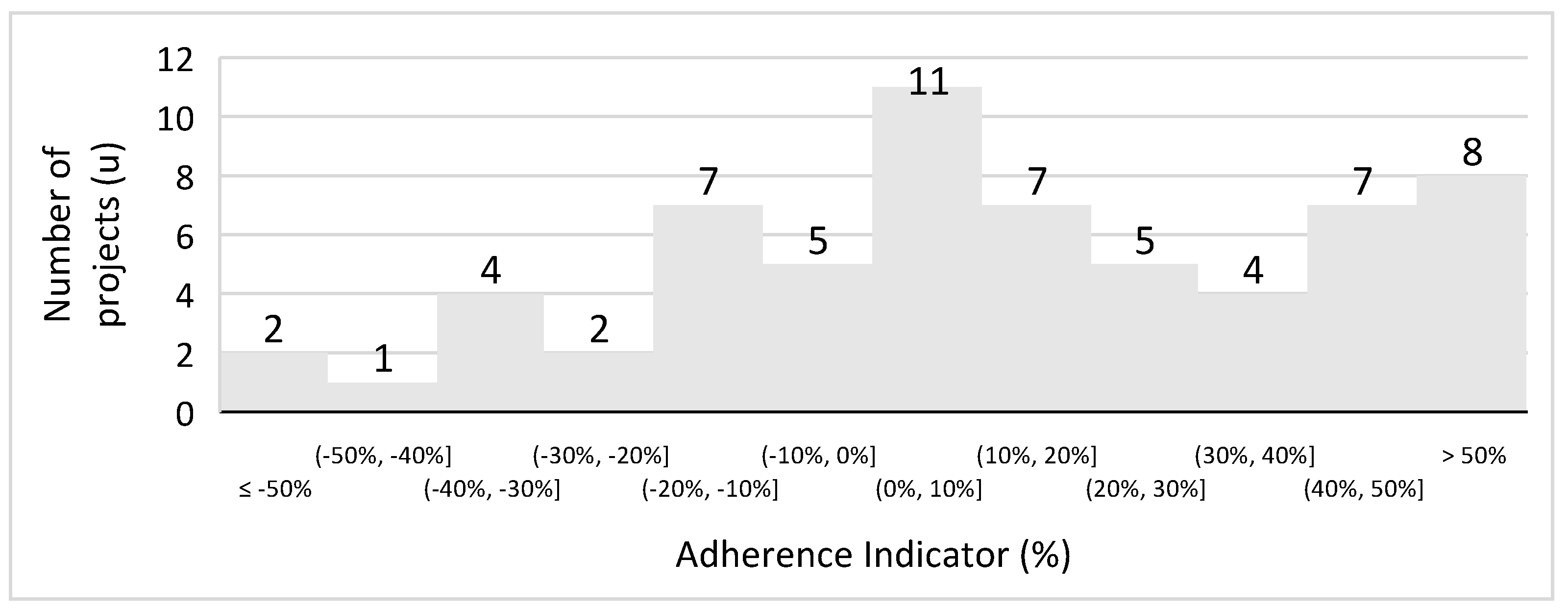
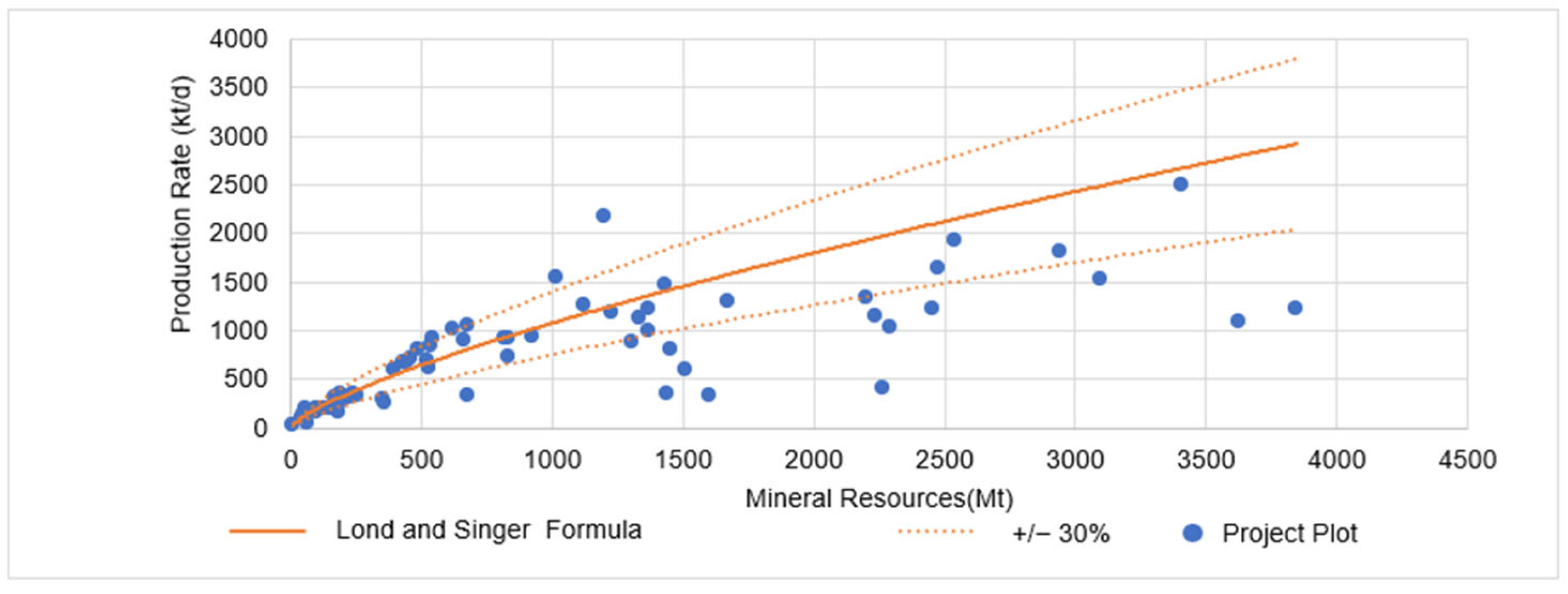
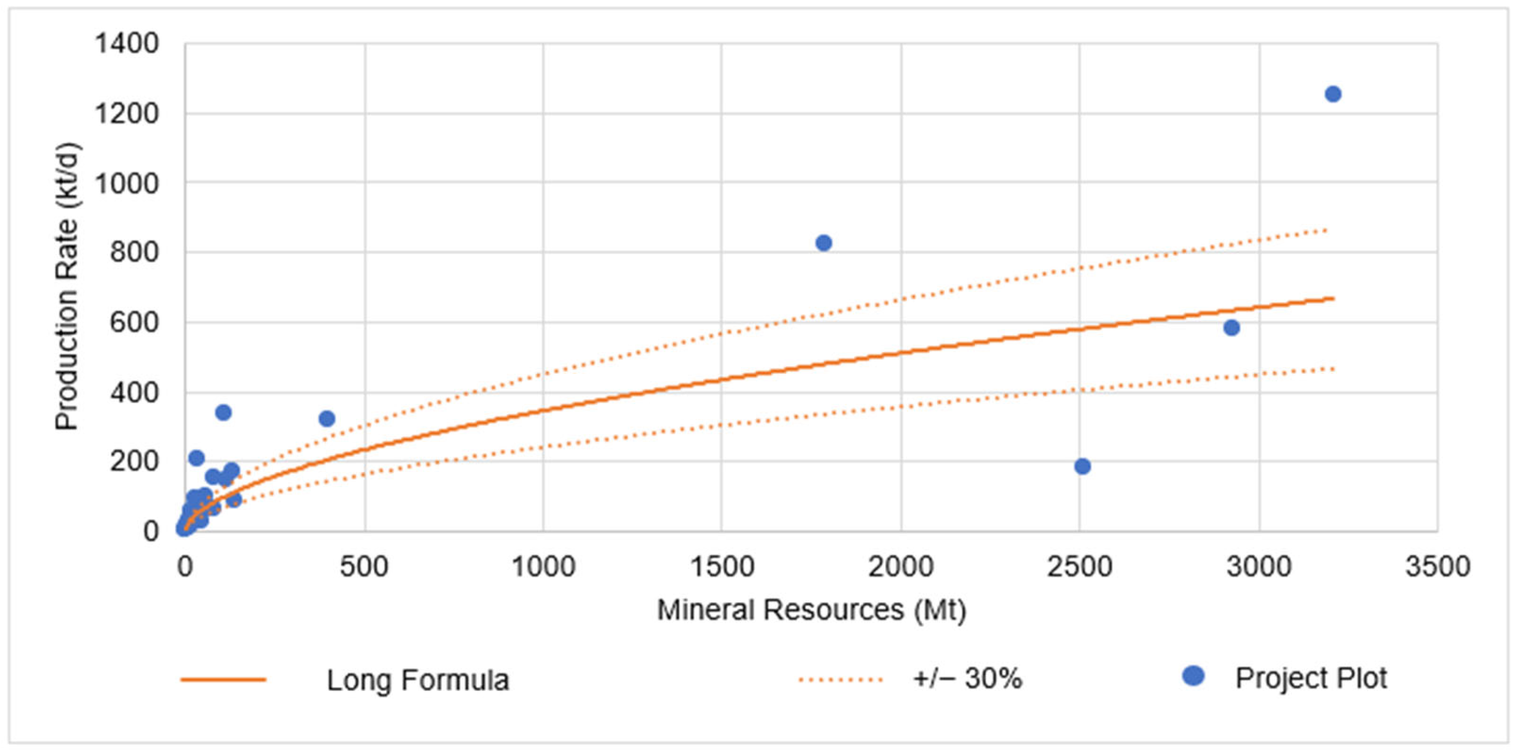
3.1. Long and Singer (2001) [4] Formula Adherence

The first validation to be performed was with the formula generated by Long and Singer [4], which estimates an equation for the production rate of open-pit copper mining projects. This formula was chosen for the adherence test because it considers open-pit copper mining projects, which are particularities included in the database used; thus, it provides a more correlated comparison. The formula created can be seen in Equation (1):

Cst = 0.0236 × Tst^0.74

(1)

where

• Cst represents the productive capacity, in short tons per day;
• Tst represents the ore mass, in short tons.

A total of 63 open-pit copper mining projects were selected to evaluate the formula. Despite Long and Singer’s [4] use of short tons in their formula, the conversion to metric tons does not affect the calculations, as the values are proportionally equivalent on both sides of the equation, preserving the outcome. The 63 projects can be reviewed in Appendix A. For these projects, we compared the daily production rates calculated using Long and Singer’s [4] formula with the actual rates from the project database. The percentage differences were then plotted in a histogram to analyze the performance of the equation. The histogram can be seen in Figure 1.

The histogram shows that many projects exhibited significant value differences compared to the formula created by Long and Singer [4]. To assess the adherence of Long and Singer’s [4] formula, a chart was created that distinctly identifies the projects that fall within the 30% variance threshold, both above and below the equation’s predictions. The results can be seen in Figure 2.

Figure 3 allows us to observe that a portion of the projects exhibit a value discrepancy greater than 30% relative to the production rate. To clarify the equation’s adherence, we calculated the number of projects with a difference of less than 30%. Out of the 63 projects analyzed, 37 exhibited a variance within this range. Consequently, Long and Singer’s [4] formula demonstrates a 59% adherence rate to the analyzed database for open-pit copper mining projects. The statistical measures calculated for this sample space were as follows: mean = 13%, standard deviation = 33%, and standard error = 4%. The standard deviation of close to 30% validates the adherence of around 59%, despite the mean being somewhat distant from zero.

3.2. Long (2009) [22] Formula Adherence—Open-Pit and Block Caving

The next formula tested for adherence against the database was Long’s [22] equation. This formula was applied to evaluate open-pit mining projects in general, without differentiating by mineral type, and also included underground projects employing block caving—a method characterized by its large-scale production, comparable to open-pit mining in terms of output. Consequently, the researchers believed that it could be relevant for estimating production rates across both mining types. This particular formula was selected to gauge the adherence of open-pit mining projects within the database, and it can be seen in Equation (2):

C = 0.123 × T^0.649

(2)

where

• C represents the productive capacity per day;
• T represents the ore mass.

To calculate a representative adherence, projects involving open-pit mining of copper, zinc, and lead were chosen and can be reviewed in Appendix A. A total of 88 open-pit copper, zinc, and lead mining projects were selected to evaluate the formula. A histogram, as represented in Figure 3, was created to analyze the comparison of Long’s [22] formula and the database.

The histogram reveals that a significant number of projects exhibit a discrepancy exceeding 30% between the values calculated using Long’s [22] equation and the actual project values. Despite incorporating zinc and lead projects into the analysis, the new equation did not result in improved adherence. Furthermore, as illustrated by the scatter plot in Figure 4, numerous projects do not fall within the defined 30% adherence margin.

After analyzing the graph, the adherence of Long’s [22] formula to the calculated production rates of the projects was assessed. Compared to the previous formula, there was a decrease in adherence: the former formula had an adherence of 59%, while the latter showed 53%, representing a 6% reduction. This difference from the previous analysis can also be explained by the statistical measures. For this sample space, the values were as follows: mean = 4%, standard deviation = 38%, and standard error = 4%. The increase in standard deviation corresponds to the reduction in the adherence indicator.

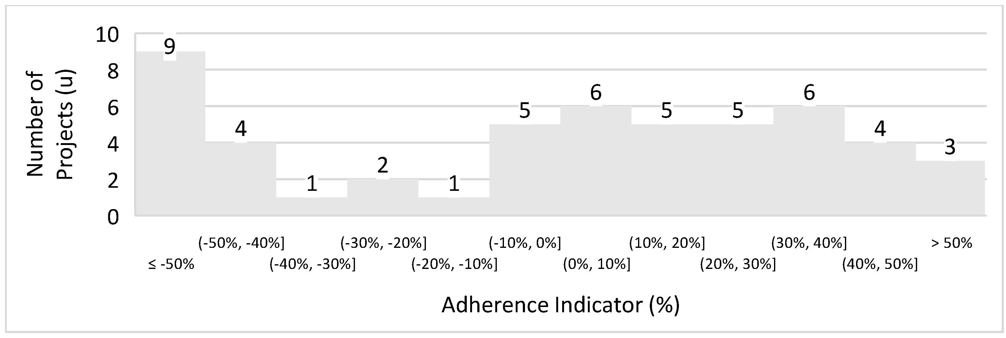
3.3. Long (2009) Formula Adherence—Underground Mining

The final equation to be assessed for adherence was Long’s [22] formula for underground mining. This formula does not include block caving mining projects, which have production rates similar to those of open-pit mining. The researchers did not specify any restrictions regarding the type of mineral for this equation. To maintain consistency, all underground mining projects from the compiled database were considered, encompassing copper, zinc, and lead minerals. The equation used for the adherence calculation is shown in Equation (3):

C = 0.297 × T^0.563

(3)

where

• C represents the productive capacity per day;
• T represents the ore mass.

A total of 51 underground copper, zinc, and lead mining projects were selected to evaluate the formula and can be reviewed in Appendix A. A histogram was created to analyze the comparison of Long’s [22] underground projects formula and the database. Figure 5 displays the histogram.

The histogram clearly shows that a large number of projects have a discrepancy greater than 30%, indicating low adherence. The scatter plot in Figure 6 illustrates how the project production rates compare to Long’s [22] formula for underground projects and how they align with the 30% margin considered for this study.

The graph analysis reveals a concentration of projects with mineral resources up to 100 million tons and few projects with a large quantity of mineral resources. The graph also enables the calculation of the adherence of Long’s [22] equation for underground mining to the projects. It can be concluded that the adherence of the underground mining projects for copper, zinc, and lead to Long’s [22] equation is 47%. This represents the lowest adherence rate calculated among all comparisons. This low adherence can also be explained by the statistical measures. This sample space had the worst statistical correlation among the samples, with the following values: mean = −11%, standard deviation = 67%, and standard error = 9%. These calculations indicate that the lower the standard deviation, the higher the adherence indicator to the formula.

With the adherence calculations performed using the three existing formulae—Long and Singer’s [4] for open-pit copper mining, Long’s [22] for open-pit and block caving mining, and Long’s [22] for underground mining—a comparison was made against the entire database, which includes both open-pit and underground mining projects for copper, zinc, and lead. These analyzed formulae are commonly used in conceptual projects to estimate the production rate. Therefore, adherence indicators with values higher than those found in the initial parametrization can be considered representative and applicable to the industry, according to the methodology defined for this study as a strategic approach.

Taylor’s [1,23] and Camm’s [23] formulae were not used because they are very generic, encompassing all types of mining methods and commodities, and would not provide the expected representativeness for the database. Singer, Menzie, and Long’s [3] formula was also excluded because it was based on gold and silver mines, and these commodities were not included in the database. Finally, Singer, Menzie, and Long’s [2] formula was not applied because it is specific to underground mining of large sulfide deposits and cannot be compared or related to the database used.

3.4. Estimation of Production Rates for Copper, Zinc, and Lead Projects

Taylor formulated an approach to estimate production rates without considering specific factors such as ore type, project scale, or mining method, in contrast to Long and Singer, who tailored their equation to particular mining methods and commodities. This study conducted a comprehensive analysis across all available variables in the database to discern patterns of adherence with varying mining types, commodities, and production volumes. The projects can be reviewed in Appendix A.

The initial analysis encompassed all projects from the database, without discrimination based on mining method, commodity type, or production volume. This step aimed to assess the consistency of adherence with previously estimated equations. By examining mineral resources in tons and daily production rates in tons, a scatter plot was generated to explore the relationships between these variables. The intent was to establish whether they exhibit statistical correlation and can inform the development of a power regression equation that improves adherence for the projects under review, surpassing the accuracy of prior formulae. The chart can be viewed in Figure 7.

In Figure 7, the distribution of projects is depicted, with mineral resources plotted on the x-axis in millions of tons and the daily production rates on the y-axis in tons. Additionally, the figure shows the trend curve resulting from a power regression analysis of the data, which includes a 30% allowable variation above and below the equation. This power regression was calculated using the least squares method. The trend curve is derived from Equation (4):

C = 0.0172 × T^0.7384

(4)

where

• C represents the productive capacity per day;
• T represents the ore mass.

The regression analysis produced a coefficient of determination (R² value), which measures the fit of the trend curve to the data. The R² value of 0.7066 means that approximately 70.66% of the variability in the dependent variable (C) can be explained by the model’s independent variable (T). This is a relatively high R² value, indicating a good fit of the model to the data. To assess the magnitude of these differences and their adherence to the study’s acceptable variation, they were represented in a histogram. This visualization helps determine whether the differences fall within the study’s acceptable 30% variation range. The histogram can be reviewed in Figure 8.

The histogram reveals that a significant number of projects deviate beyond the 30% variance threshold considered for formula adherence. Of the 160 projects evaluated, 89 remained within the acceptable 30% margin of the production rate differences calculated by the equation compared to the project’s reported values. This equates to an adherence rate of 56%. While this rate is comparable to those achieved with previous formulae, it falls short of being considered satisfactory by the adherence comparison methodology. The analysis of the statistical measures reinforces the low statistical relationship of the sample space. The values are as follows: mean = −13%, standard deviation = 76%, and standard error = 6%.

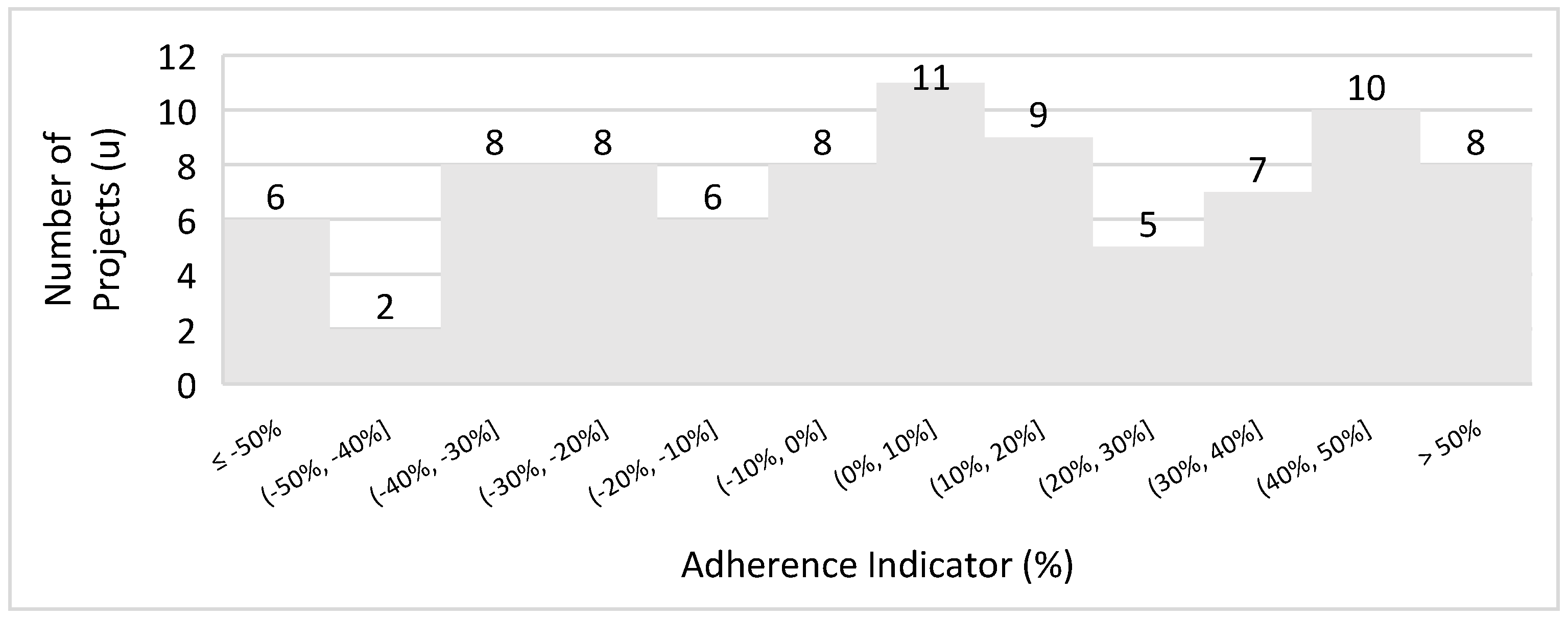
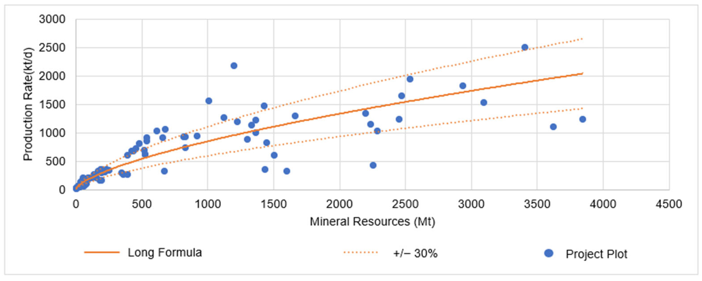
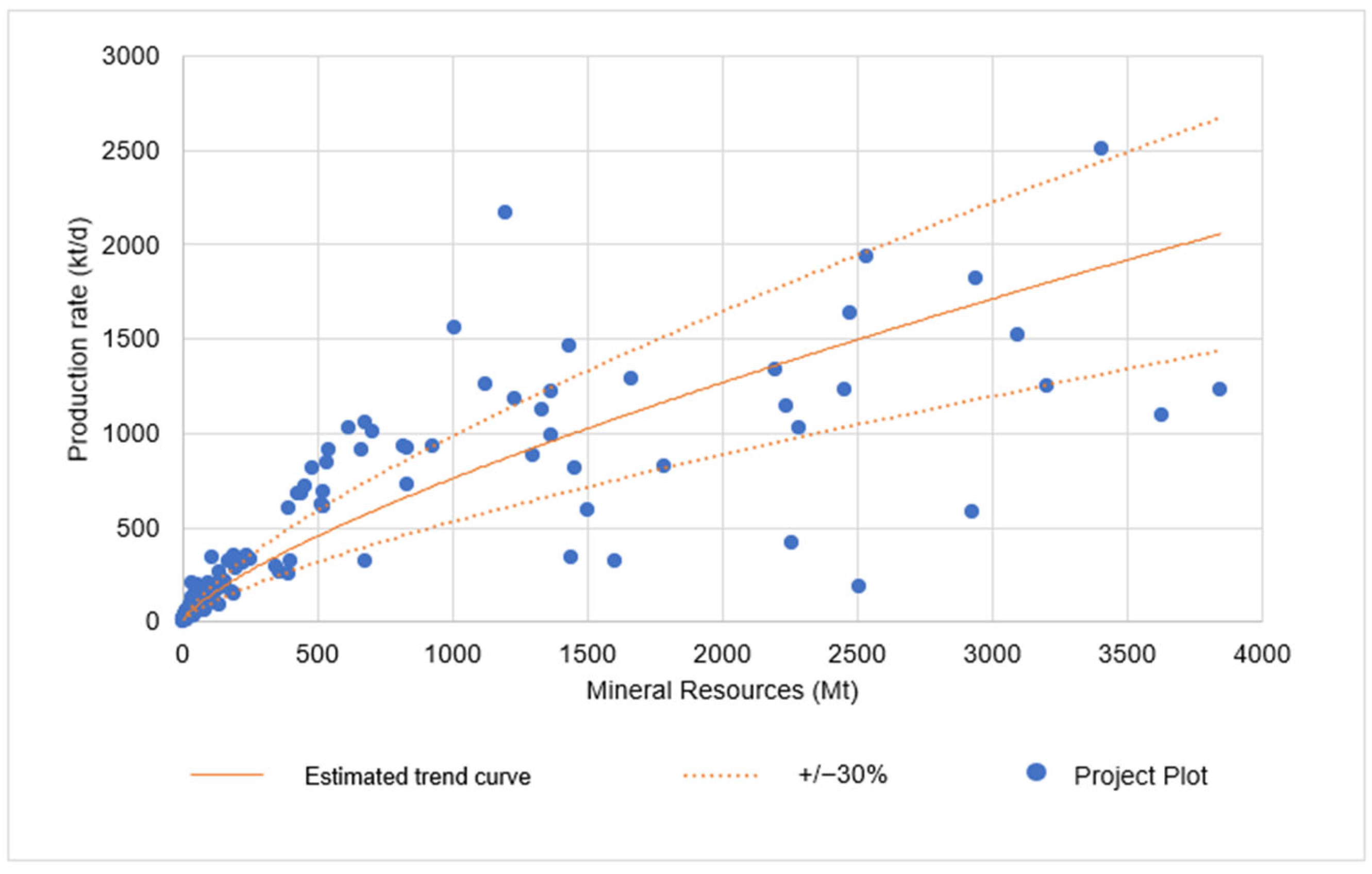
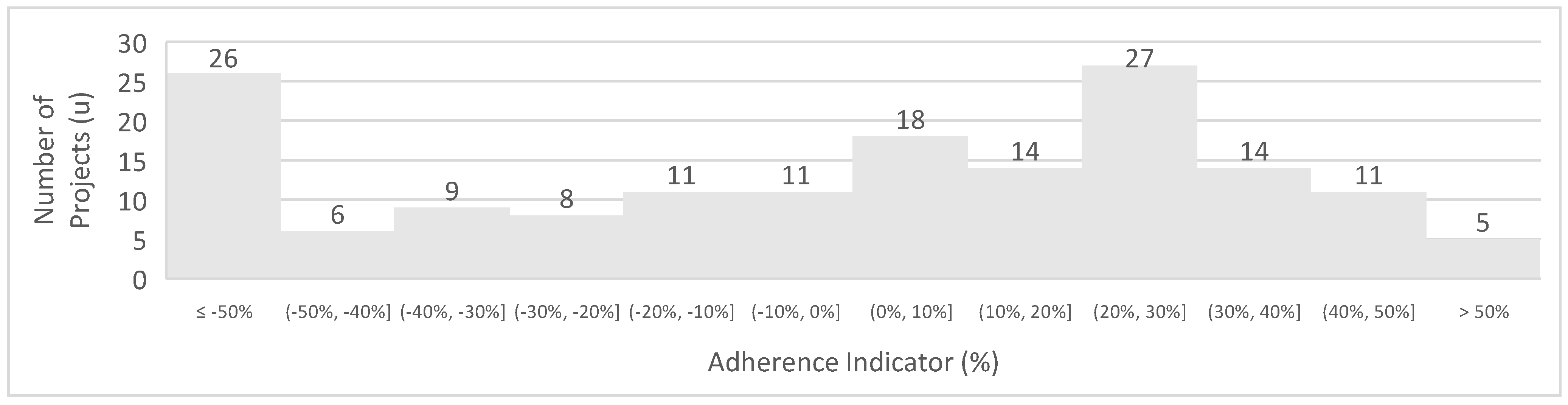
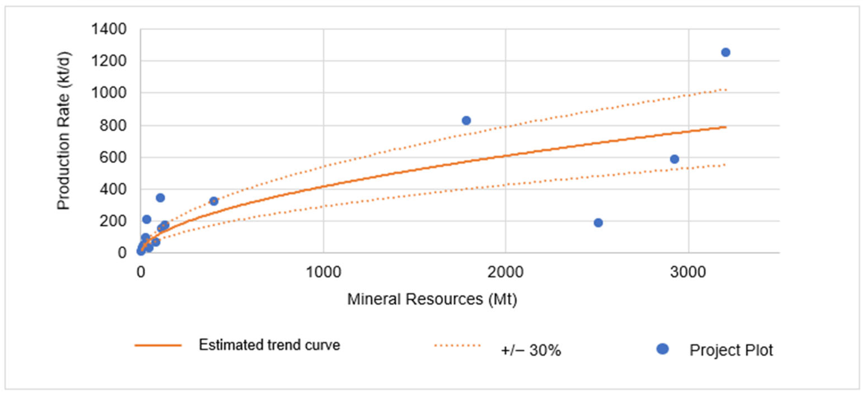
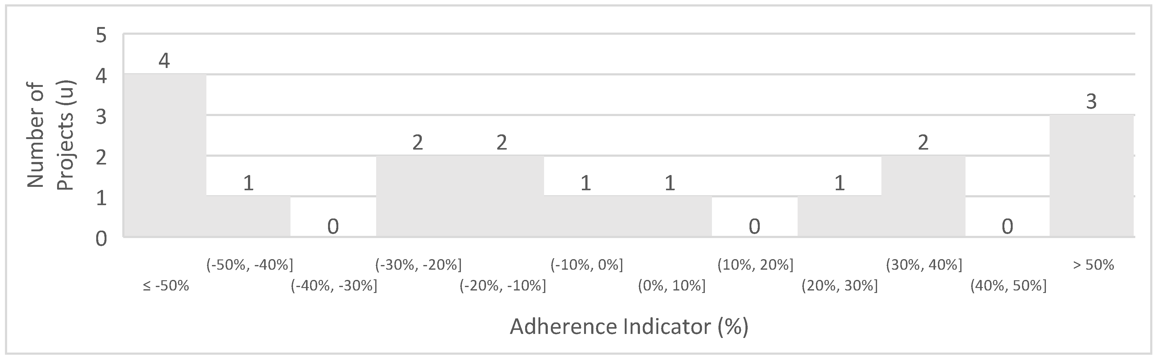
3.5. Estimation of Production Rates for Open-Pit Copper Projects

To enhance the fit of the formulae to the database for copper, zinc, and lead mining projects, power regression modifications were performed. These adjustments aimed to refine the database categorization by mining method and mineral type, resulting in a more consistent and less variable regression curve.

The initial regression modification examined open-pit copper mining projects. A subset of 63 projects fitting these criteria was analyzed and can be reviewed in Appendix A. For these projects, a scatter plot was created using the variables of mineral resources in tons and production rates in tons per day. The graph facilitated an analysis of the correlation between the samples, leading to the generation of a trend curve through power regression, from which an equation was derived. Figure 9 illustrates the trend curve produced by the power regression, allowing for the identification of projects that fall within the adherence range, accounting for a 30% variation above or below the calculated value.

The regression analysis produced a coefficient of determination (R² value). The R² value of 0.5978 indicates reasonable accuracy; though not as high as the previous equation’s value, the equation remains statistically significant despite its variability. The trend is represented by Equation (5):

C = 0.1449 × T^0.639

(5)

where

• C represents the productive capacity per day;
• T represents the ore mass.

Applying Equation (5), we recalculated the daily production rates using the projects’ mineral resources. The resulting percentage differences from the projects’ original production rates were then plotted in a histogram to visualize the distribution of these variances. The histogram can be analyzed in Figure 10.

Analysis of the histogram reveals that numerous projects fall outside the acceptable 30% variation threshold. Adherence was assessed for 63 projects; 35 met the 30% variation criterion, yielding a 56% adherence rate. This rate is consistent with the adherence calculated for the entire database, indicating no significant improvement in the formula’s reliability, even when focusing exclusively on open-pit copper mining projects. The statistical analysis proves that, for this sample space, the adherence is low. Despite the improvement in the standard deviation, it still remains high. The data are as follows: mean = −8%, standard deviation = 40%, and margin of error = 5%. Given that the equation did not improve adherence, the analysis was further refined by limiting the scope to projects with a maximum daily production of 140,000 tons, aiming for a more consistent curve and enhanced formula reliability.

Out of the 63 projects initially analyzed, 55 met the daily production limit of 140,000 tons. This subset underwent a new power regression analysis, leading to the derivation of an updated formula. Figure 11 illustrates the project distribution on the scatter plot, indicating which projects align with the study’s established 30% variation range for acceptable daily production rates.

The trend is represented by Equation (6):

C = 0.2691 × T^0.6056

(6)

where

• C represents the productive capacity per day;
• T represents the ore mass.

The graph reveals that a considerable number of projects do not meet the acceptable variation range, reflecting poor adherence. The calculated adherence rate was lower than the one derived from Equation (5), which suggests that the new curve is less representative of the database values. The histogram in Figure 12 was constructed to facilitate the adherence calculation, illustrating the variance distribution and the number of projects within each interval.

Analysis of the histogram indicates that out of the 55 projects considered for the power regression-derived Equation (6), only 28 remained within the acceptable range of variation from the calculated to the actual daily production rates. Consequently, the adherence rate to Equation (6) stands at 51%, which is lower than the rate achieved when including all projects. The statistical analysis showed a slight improvement compared to the previous analysis by reducing the standard deviation, but it still had high values, as follows: mean = −5%, standard deviation = 35%, and standard error = 9%. This finding suggests that the new equation does not offer an improvement in formula reliability. Data analysis from this study on open-pit copper mining projects did not yield any enhancement in the equation’s reliability over the previous research by Taylor and Long.

3.6. Estimation of Production Rates for Underground Copper Projects

The production rate estimates for open-pit copper projects did not yield better adherence than previous studies’ formulae, prompting an investigation into production rate estimates for underground copper mining. The utilized database comprises 17 copper projects with underground mining operations. Using these data, a scatter plot was generated to analyze the relationship between the mineral resources and the calculated production rates, leading to the development of a new trend curve and formula. The curve can be analyzed in Figure 13.

The graph yielded a regression curve. From this curve, it is possible to analyze the discrepancies between the project’s actual daily production rates in tons and those predicted by the regression. The R² value of 0.656 indicates reasonable accuracy and that the equation remains statistically significant. The regression curve is represented by Equation (7):

C = 0.4736 × T^0.5492

(7)

where

• C represents the productive capacity per day;
• T represents the ore mass.

A histogram was constructed to facilitate the adherence calculation, illustrating the variance distribution and the number of projects within each interval. This histogram can be analyzed in Figure 14.

The histogram indicates that among the 17 evaluated projects, only 7 meet the acceptable 30% variation range when comparing the calculated daily production rates to the project’s actual rates. This results in an adherence rate of 41%, which is lower than previous studies and suggests limited representativeness of Equation (7). The statistical analysis also shows a low representativeness of the sample space, presenting the following values: mean = −21%, standard deviation = 78%, and standard error = 19%. Observations from the scatter plot highlighted substantial fluctuations in the production rates. To improve the correlation between the studied variables, the analysis was refined to include only projects with daily production rates of up to 10,000 tons. The updated scatter plot is depicted in Figure 15.

The trend curve depicted in Figure 15 corresponds to Equation (8):

C = 0.7741 × T^0.5044

(8)

where

• C represents the productive capacity per day;
• T represents the ore mass.

Equation (8) lacks statistical significance, as the data points are notably distant from the resulting curve, despite the small sample size and the R² value of 0.2704.

Analysis revealed that among the eight underground copper mining projects with daily production under 10,000 tons, only half adhered to the acceptable 30% variance between the actual project values and those predicted by the developed equation. This resulted in an adherence rate of 50%, which is lower than the rates achieved in previous studies. Despite showing a slight improvement in the statistical analyses, the standard deviation remained high. The values were as follows: mean = −10%, standard deviation = 52%, and standard error = 18%. Considering these results, neither open-pit nor underground copper mining projects demonstrated adherence improvements over those found in prior research, and these equations should not be used as reference for future studies.

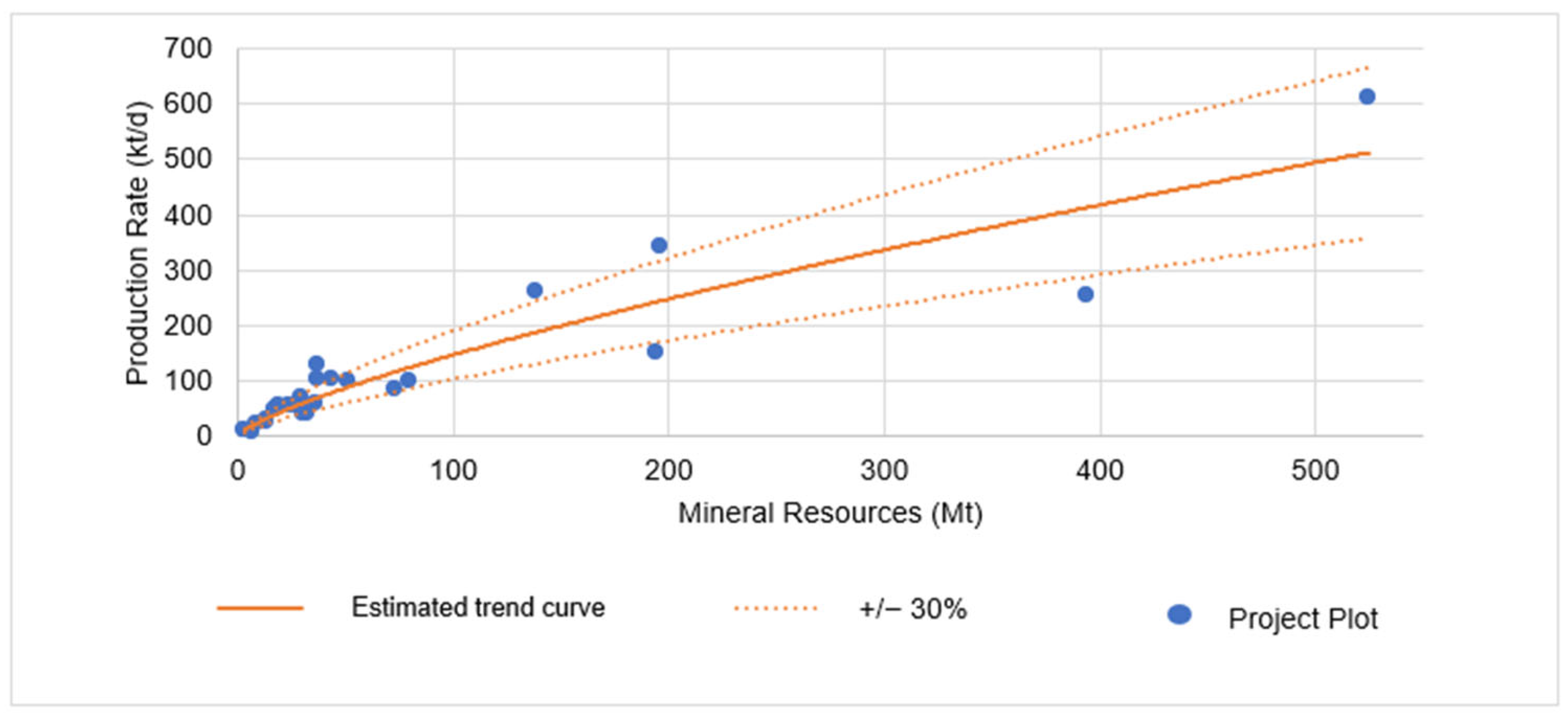
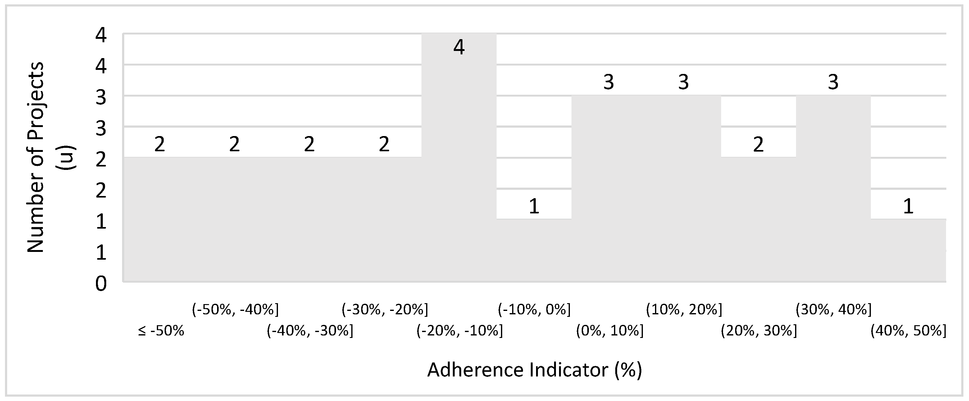
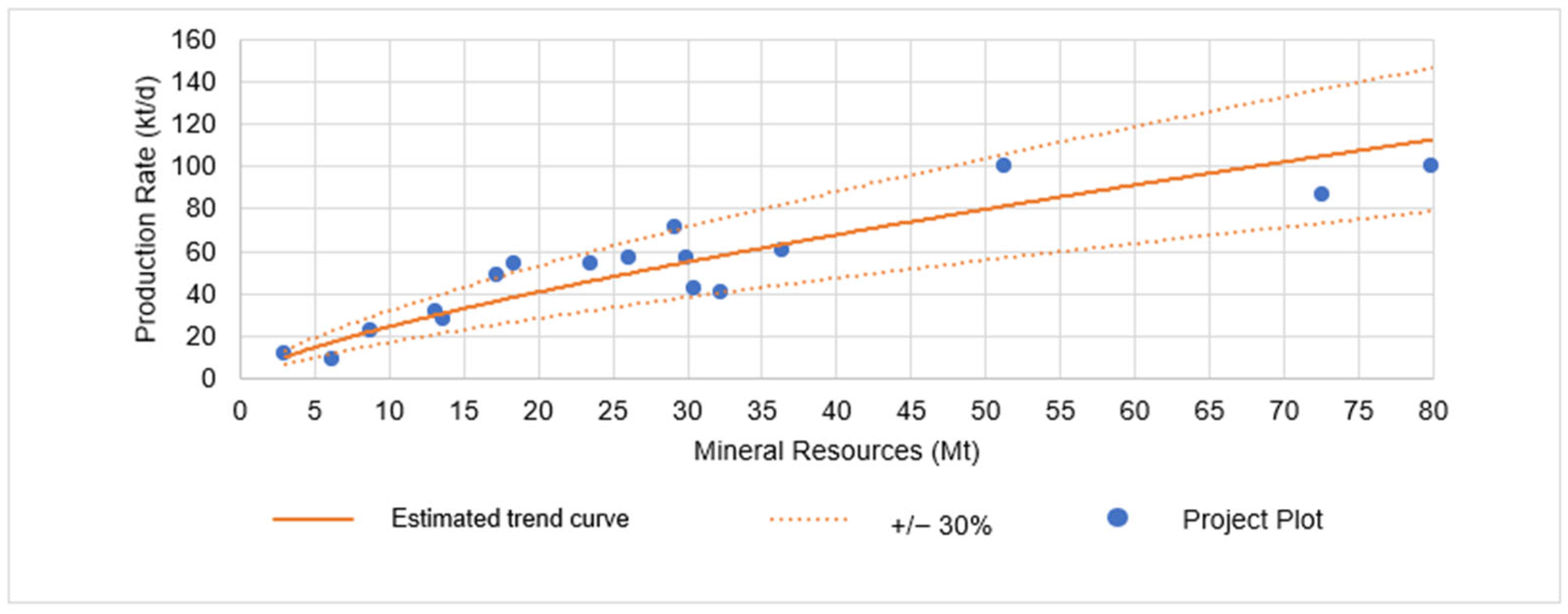
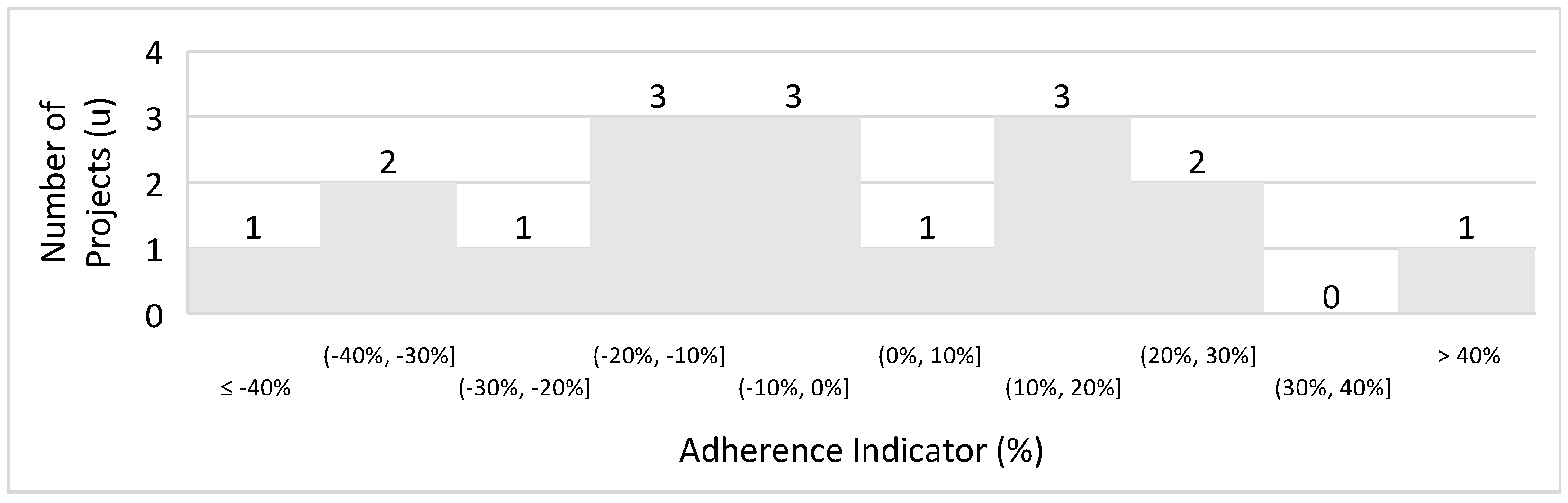
3.7. Estimation of Production Rates for Open-Pit Zinc and Lead Projects

Most zinc projects are commonly linked with lead mineralization, and in the database used, numerous projects involve both zinc and lead. Mudd et al. [24] noted the frequent co-occurrence of these minerals in deposits. Therefore, the decision was made to analyze zinc and lead together due to their production rate similarities. Projects for both minerals were separately examined for open-pit and underground mining, mirroring the approach taken for copper. The analysis of production rate estimates for open-pit zinc and lead projects encompassed 25 projects, focusing on two key variables: mineral resources in tons, and daily production rates in tons. The analysis of the 25 projects resulted in a scatter plot, presented in Figure 16 for review.

The graph analysis reveals that numerous projects are within the acceptable 30% variance from the equation-derived values. The R² value of 0.8426 indicates a robust regression, demonstrating a strong correlation between the data and the formulated equation.

The trend is represented by Equation (9):

C = 0.0141 × T^0.7423

(9)

where

• C represents the productive capacity per day;
• T represents the ore mass.

The difference was calculated between the daily production rates, as predicted by Figure 16 using the projects’ reported mineral resources, and the projects’ originally calculated production figures. A histogram was constructed to clearly display the distribution of the calculated differences among the projects, as shown in Figure 17.

The histogram shows a majority of the projects falling within the acceptable variance range, demonstrating strong adherence to the equation. With 15 out of 25 projects meeting the adherence criteria, the adherence rate stands at 60%. Figure 15 surpasses the adherence rates of previous studies, underscoring the equation’s relevance and its ability to correlate the data across projects. The statistical analyses confirm the good adherence of the formula to the sample space. For this case, the values obtained are as follows: mean = −5%, standard deviation = 33%, and standard error = 7%. The calculations show that both the mean and the standard deviation have satisfactory values. The standard deviation is very close to the adherence variation of 30%.

Upon examining the scatter plot in Figure 16, a notable concentration of projects with daily production rates under 10,000 tons is observed, exhibiting improved adherence to the equation, as noted in Figure 17. In pursuit of a formula with superior adherence, the projects were filtered to include only those with production rates of up to 10,000 tons per day.

These selected projects were then depicted in a scatter plot, with mineral resources in tons on the x-axis and daily production rates in tons on the y-axis. The graph features a trend curve from a power regression analysis, which led to the formulation of Equation (10), and also illustrates the 30% variance intervals around the y-values. The scatter plot can be visualized in Figure 18.

Figure 18 shows that the majority of projects align with the 30% variance interval curves. The coefficient of determination (R² value) measures the accuracy of the curve against the database and yielded a value of 0.8296. This value denotes a strong regression, implying a close alignment between the data and the derived equation. The trend is represented by Equation (10):

C = 0.0191 × T^0.7302

(10)

where

• C represents the productive capacity per day;
• T represents the ore mass.

The daily production rates of the 17 zinc and lead projects, each with a production below 10,000 tons, were re-estimated using the new equation based on their reported mineral resources. A histogram, shown in Figure 19, illustrates the variance between the original production rates of the projects and the rates derived from the new equation.

The histogram indicates that 13 of the 17 projects adhere to the acceptable variance range, yielding an impressive 76% adherence rate to the formula. This rate surpasses those found in prior studies, reflecting a robust correlation with the trend curve. The new equation is thus shown to be relevant, with a significant correlation between mineral resources and daily production rates. To confirm the good correlation of the formula, the following statistical measures were calculated: mean = −3%, standard deviation = 24%, and standard error = 6%. Open-pit zinc and lead mining projects exhibited higher adherence rates than those of copper projects and surpassed the findings of earlier research by other scholars.

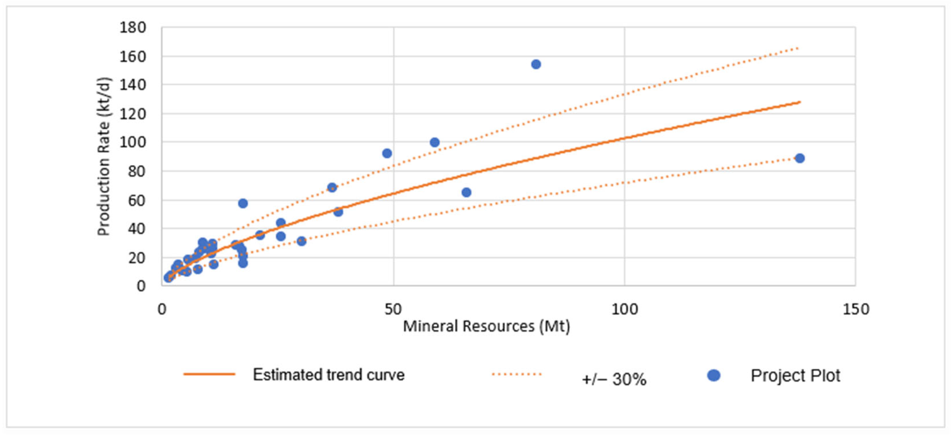
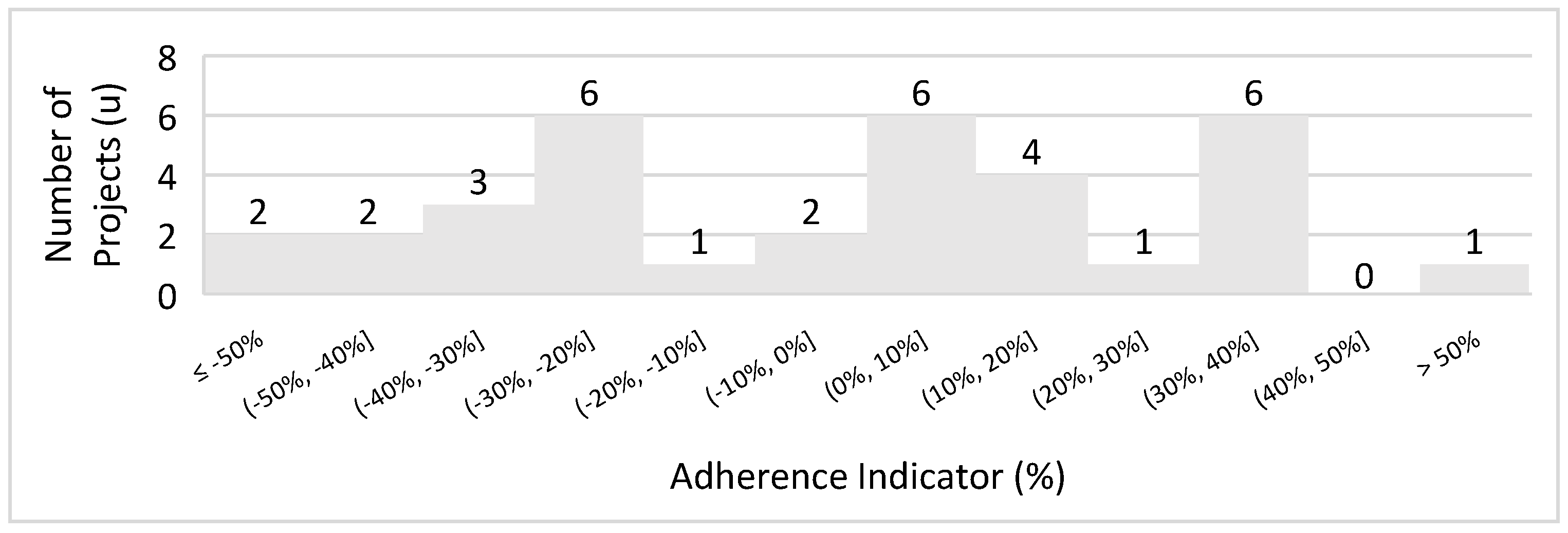
3.8. Estimation of Production Rates for Underground Zinc and Lead Projects

Zinc and lead projects showed good adherence to the formulae derived from open-pit mining data. Similarly, an analysis was conducted for the production rate estimates of underground zinc and lead mining projects, which totaled 34. The two key variables to be examined were the mineral resources in tons and the projects’ daily production rates in tons. These variables were plotted on a scatter plot, represented in Figure 20, with the mineral resources in tons on the x-axis and the daily production rates in tons per day on the y-axis.

The graph features a trend curve for the projects, encompassing a 30% variation for the production rates. It highlights the projects within the acceptable variation range. The majority of projects align with the acceptable range, indicating good adherence to the curve. Figure 20 presents the trend curve, defined by Equation (11):

C = 0.0408 × T^0.6751

(11)

where

• C represents the productive capacity per day;
• T represents the ore mass.

This curve enables the estimation of daily production rates and the assessment of project adherence by comparing the original and recalculated production rate values. The R² value or coefficient of determination of 0.722 confirms a solid regression, showing that the data are well correlated with the equation and are statistically sound. The histogram in Figure 21 was constructed to better illustrate the variance distribution.

The histogram enables the calculation of adherence for the new equation; of the 34 projects, 20 fall within the acceptable range for this study. This results in an adherence rate of 59%, which is considered good, as it yields more satisfactory outcomes than the equations from previous studies. The statistical analysis is consistent with the adherence results, presenting the following values: mean = −5%, standard deviation = 33%, and standard error = 6%. It can be noted that when the standard deviation is below 33%, the adherence values are satisfactory.

Analysis of Figure 18 indicates a clustering of projects with production rates of up to 5200 tons per day. In pursuit of a more adherent formula, the projects were filtered to cap daily production at 5200 tons. These selected projects are depicted in a scatter plot in Figure 22, where the x-axis represents mineral resources in tons and the y-axis shows daily production rates. The plot includes a trend curve from a power regression that produced an equation, along with 30% variance intervals around the y-values.

Figure 22 presents the trend curve defined by Equation (12):

C = 0.1954 × T^0.5743

(12)

where

• C represents the productive capacity per day;
• T represents the ore mass.

The daily production rates of the 27 underground zinc and lead projects, each with outputs under 5200 tons, were re-estimated using the mineral resources data and the trend curve. The histogram shown in Figure 23 illustrates the variance between the original production rates of the projects and the rates derived from the new equation for clearer comparison.

The histogram indicates that 19 of the 27 projects are within the acceptable range of variance, yielding a high adherence rate of 70% to the formula. This rate is an improvement over previous studies, reflecting a strong correlation with the trend curve. The new equation proves to be significant, showing a meaningful relationship between mineral resources and daily production rates. The analysis of the statistical measures reinforces the good adherence of the sample space to the formula. The values found were as follows: mean = −3%, standard deviation = 26%, and standard error = 5%.

Underground zinc and lead projects have shown that their formulae align well with the projects’ actual data, indicating that these trend curves could be effectively used for initial production rate estimations. This study aimed to develop a reliable equation to accurately size production rates and the lifespan of early-stage mining projects for copper, zinc, and lead. Copper and zinc are currently considered strategic due to their importance in the new energy matrix focused on decarbonization and renewable energies, while lead plays a supporting role, particularly in energy storage applications.

Furthermore, this work seeks to assist other mining companies and consultancies in quantifying production rates and project lifespans appropriately during the initial study phases, thereby avoiding unnecessary expenses and time loss in the development of conceptual projects. Using the proposed methodology, this study successfully parameterized the database with the previous formulae created by Long and Singer [4] and Long [22] for open-pit and underground mines. The database adherence to these formulae ranged from 47% to 59%, with the highest value pertaining to Long and Singer’s formula [4]. Therefore, any value equal to or less than these would indicate an unsatisfactory and irrelevant formula for future projects. This study also determined the relationships between the adherence indicator and the standard deviation of the analyzed sample spaces. The higher the adherence value, the lower the standard deviation. Additionally, it can be concluded that the set of projects with a standard deviation below 30% or very close to this value will have good adherence.

Table 6. Adherence of Long and Singer’s (2001) and Long’s (2009) formulae to the copper, zinc and lead projects in the database.

Source (Year)	Equation	Mining Method	Number of Evaluated Projects	Adherence (%)	Standard Deviation
Long and Singer (2001) [4]	Cst = 0.0236 × Tst0.74	Open-pit (copper)	63	59%	33%
Long (2009) [22]	C = 0.123 × T0.649	Open-pit/block caving	88	53%	38%
Long (2009) [22]	C = 0.297 × T0.563	Underground (except block caving)	51	47%	67%

Source: Authors.

summarizes the values found per formula.

This study concluded that using a more generic database without considering separation by mining method and/or commodities does not yield good adherence results. This was evident with the equation including all 160 evaluated projects, which, despite being based on a large number of projects to generate the curve, only achieved an adherence rate of 56%, falling short of the rate achieved by Long and Singer’s formula [4]. It was also determined that segmenting the sample space by intervals of production rate values enhances the accuracy of adherence calculations.

Furthermore, it was demonstrated that the copper projects in the database do not correlate well with the generated equations, resulting in low R² values from the regressions, poor adherence of the formulae to the database, and unsatisfactory statistical measures as the standard deviations were too high. The low adherence of copper to the formulae may be linked to the more complex geological context of these projects. However, to make this assertion, further studies on this topic are necessary and could be an area for future research.

Table 7. Adherence of developed equations for copper.

Developed Equation	Mining Method	Number of Evaluated Projects	Coefficient of Determination (R2)	Adherence (%)	Standard Deviation
C = 0.1449 × T0.639	Open-pit (copper)	63	0.5978	56%	40%
C = 0.2691 × T0.6056	Open-pit (copper) up to 140 ktons/day	55	0.5762	51%	35%
C = 0.4736 × T0.5492	Underground (copper)	17	0.656	41%	78%
C = 0.7741 × T0.5044	Underground (copper) up to 10 ktons/day	8	0.27	50%	52%

Source: Authors.

provides a summary of these findings.

Zinc and lead projects, unlike copper ones, showed outstanding adherence to the developed equations, validating their use as reliable references for estimating production rates in future open-pit and underground mining projects. It is important to note that the standard deviation for zinc and lead projects remained below 33%, reaching as low as 24%. This indicates that the standard deviation of the samples is related to good adherence and aligns with this study’s methodology, which considers values within the 30% range as indicative of good adherence. The adherence rates achieved by these projects are detailed in

Table 8. Adherence of developed equations for zinc and lead.

Developed Equation	Mining Method	Number of Evaluated Projects	Coefficient of Determination (R2)	Adherence (%)	Standard Deviation
Cst = 0.0141 × Tst0.7523	Open-pit (zinc and lead)	25	0.8426	60%	33%
C = 0.0191 × T0.7302	Open-pit (zinc and lead) up to 10 ktons/day	17	0.8296	76%	24%
C = 0.0408 × T0.6751	Underground (zinc and lead)	34	0.722	59%	33%
C = 0.1954 × T0.5743	Underground (zinc and lead) up to 5.2 ktons/day	27	0.7184	70%	26%

Source: Authors.

. Additionally, it was noted that refining the database by excluding outliers significantly improved the adherence outcomes.

4. Conclusions

Firstly, a parametric analysis of the utilized database was conducted using well-established formulae from previous authors, which are widely used in the industry for this type of investigation, in order to build a baseline for the adherence indicator. This analysis revealed a direct correlation with the indicator and the standard deviation calculated for specific sample spaces, as presented in Table 6. Following this parameterization, the calculations performed for copper projects did not yield satisfactory indicators or better results than those presented by the formulae of previous authors. The calculated standard deviation also demonstrated this correlation, as specified in Table 7. This result indicates that copper projects exhibit significant variability in the relationship between the two studied variables—mineral resources and production rate—and that a satisfactory estimation of the production rate would require the inclusion of additional variables in the study. In contrast, the calculations for zinc and lead projects showed an excellent correlation between the variables mineral resources and production rate. They presented good adherence indicators and a standard deviation below 33%, as observed in Table 8.

Some additional considerations can be analyzed. The present study did not consider some variables that were evaluated by other authors, such as investment value, operational cost, mineral grades, and the specific geological context of each deposit, which aimed at estimating the production rates of mining projects. The exclusion of such factors could introduce some uncertainty regarding the new equations obtained. However, the use of an updated database with ongoing projects supports the investigation of these factors, as each analyzed project was subject to an evaluation of all of these variables to estimate the production rate presented in the database. Another important factor that was not investigated in this study, and has not been widely evaluated by other authors, is the thickness and shape of the mineral bodies. This specific factor is highly relevant for determining the production rate of new mines, but it is difficult to find in available databases, requiring case-by-case investigation. The authors of this study consider that the low adherence of copper projects is due to the variability in the thickness and shape of copper mineral bodies. Copper has disseminated and veiny formations, very thick and narrow bodies, and oxidization and sulfide mineralization, which, considering the same quantity of mineral resources, could considerably vary the production rate. Zinc and lead also exhibit these variations, but zinc and lead projects and mines predominantly have veins and sulfide mineral deposits that substantially reduce the variation in the production rate considering the same mineral resource. To substantiate these assertions, a deeper investigation into these concepts is necessary and should be conducted in future works. The authors consider the use of machine learning and artificial intelligence essential for more complex analyses of the variables and the development of more accurate estimates, and these should be present in future works to be developed.

In conclusion, the present work successfully developed a strategic approach to define the production rate in conceptual projects of critical raw materials such as zinc and lead, minerals that are very relevant to the new energy matrix. The analyzed database of the mentioned minerals generated a production rate equation with a good adherence indicator and statistical relevance in comparison with well-established formulae from previous authors using mineral resources as the basis of their estimations. These formulae will help future conceptual zinc and lead projects to be more assertive in estimating their production rates and avoid rework and excessive expenses, bringing more sustainability to the business.

References

- Taylor, H.K. Mine Evaluation and Feasibility Studies. In Mineral Industry Costs; Hoskins, J.R., Green, W.R., Eds.; Northwest Mining Association: Reno, Nevada, 1977; pp. 1–17. [Google Scholar]
- Singer, D.A.; Menzie, W.D.; Long, K.R. A Simplified Economic Filter for Underground Mining of Massive Sulfide Deposits; USGS: Pt. Reyes, CA, USA, 2000. [Google Scholar]
- Singer, D.A.; Menzie, W.D.; Long, K.R. A Simplified Economic Filter for Open-Pit Gold-Silver Mining in the United States; USGS: Pt. Reyes, CA, USA, 1998. [Google Scholar]
- Long, K.R.; Singer, D.A. A Simplified Economic Filter for Open-Pit Mining and Heap-Leach Recovery of Copper in the United States; USGS: Pt. Reyes, CA, USA, 2001. [Google Scholar]
- Mariz, J.L.V.; de Lemos Peroni, R. Estimativa de Taxa de Produção Em Fases Prematuras de Projeto Através de Dados Segmentados Por Substância Mineral, Método de Lavra e Porte Dos Empreendimentos. In Proceedings of the 19° Simpósio de Mineração,parte integrante da ABM Week, São Paulo, Brasil, 2–4 October 2018; pp. 423–434. [Google Scholar]
- Mariz, J.L.V.; de Lemos Peroni, R. Adaptação Da Regra de Taylor à Realidade Brasileira Para Determinação Inicial Da Taxa de Produção Em Projetos Mineiros. Tecnol. Metal. Mater. Mineração 2019, 16, 1–6. [Google Scholar] [CrossRef]
- Wells, H.M. Optimization of Mining Engineering Design in Mineral Valuation. Min. Eng. 1978, 30, 1676–1684. [Google Scholar]
- Cavender, B. Determination of the Optimum Lifetime of a Mining Project Using Discounted Cash Flow and Option Pricing Techniques. Min. Eng. 1992, 44, 1262–1268. [Google Scholar]
- Lizotte, Y.; Elbrond, J. Choice of Mine-Mill Capacities and Production Schedules Using Open Ended Dynamic Programming. CIM Bull. 1982, 75, 154–163. [Google Scholar]
- Smith, L.D. A Critical Examination of the Methods and Factors Affecting the Selection of an Optimum Production Rate. CIM Mag. Bull. 1997, 90, 48–54. [Google Scholar]
- Baruti, K.R. Developed Regression Models of Mining Rate Fit on Resource and Reserve Variations in Gold Mining. Int. J. Eng. Innov. Res. 2018, 7, 159–165. [Google Scholar]
- Sabour, S.A.A. Mine Size Optimization Using Marginal Analysis. Resour. Policy 2002, 28, 145–151. [Google Scholar] [CrossRef]
- Souza, F.R.; Câmara, T.R.; Torres, V.F.N.; Nader, B.; Galery, R. Optimum Mine Production Rate Based on Price Uncertainty. REM—Int. Eng. J. 2019, 72, 625–634. [Google Scholar] [CrossRef]
- Northey, S.; Mohr, S.; Mudd, G.M.; Weng, Z.; Giurco, D. Modelling Future Copper Ore Grade Decline Based on a Detailed Assessment of Copper Resources and Mining. Resour. Conserv. Recycl. 2014, 83, 190–201. [Google Scholar] [CrossRef]
- Michaux, S.P. Estimation of the Quantity of Metals to Phase out Fossil Fuels in a Full System Replacement, Compared to Mineral Resources. Bulletin 2024, 416, 1–293. [Google Scholar] [CrossRef]
- Tabelin, C.B.; Park, I.; Phengsaart, T.; Jeon, S.; Villacorte-Tabelin, M.; Alonzo, D.; Yoo, K.; Ito, M.; Hiroyoshi, N. Copper and Critical Metals Production from Porphyry Ores and E-Wastes: A Review of Resource Availability, Processing/Recycling Challenges, Socio-Environmental Aspects, and Sustainability Issues. Resour. Conserv. Recycl. 2021, 170, 105610. [Google Scholar] [CrossRef]
- Natural Resources Canada. The Canadian Critical Minerals Strategy from Exploration to Recycling: Powering the Green and Digital Economy for Canada and the World; Natural Resources Canada: Ottawa, ON, Canada, 2022; ISBN 9780660463391.
- de Castro, F.F.; Peiter, C.C.; Góes, G.S. TD 2768—Minerais Estratégicos e Críticos: Uma Visão Internacional e Da Política Mineral Brasileira. Texto para Discussão 2022, 2768, 1–40. [Google Scholar] [CrossRef]
- Hickson, R.J.; Owen, T.L. Project Management for Mining: Handbook for Delivering Project Success, 2nd ed.; Society for Mining Metallurgy and Exploration (SME): Englewood, CO, USA, 2022; ISBN 9780873354943. [Google Scholar]
- Hickson, R.J.; Owen, T.L. Project Management for Mining: Handbook for Delivering Project Success; Society for Mining Metallurgy and Exploration (SME): Englewood, CO, USA, 2015; ISBN 9780873354035. [Google Scholar]
- Mariz, J.L.V. Análise Da Aderência Dos Métodos de Previsão Da Taxa de Produção Em Fases Prematuras de Projetos Mi-Neiros à Realidade Brasileira; Universidade Federal do Rio Grande do Sul: Rio Grande, Brazil, 2018. [Google Scholar]
- Long, K.R. A Test and Re-Estimation of Taylor’s Empirical Capacity-Reserve Relationship. Nat. Resour. Res. 2009, 18, 57–63. [Google Scholar] [CrossRef]
- Camm, T.W. Simplified Cost Models for Prefeasibility Mineral Evaluations; USGS: Pt. Reyes, CA, USA, 1991. [Google Scholar]
- Mudd, G.M.; Jowitt, S.M.; Werner, T.T. The World’s Lead-Zinc Mineral Resources: Scarcity, Data, Issues and Opportunities. Ore Geol. Rev. 2017, 80, 1160–1190. [Google Scholar] [CrossRef]
Disclaimer/Publisher’s Note: The statements, opinions and data contained in all publications are solely those of the individual author(s) and contributor(s) and not of MDPI and/or the editor(s). MDPI and/or the editor(s) disclaim responsibility for any injury to people or property resulting from any ideas, methods, instructions or products referred to in the content. |
© 2025 by the authors. Licensee MDPI, Basel, Switzerland. This article is an open access article distributed under the terms and conditions of the Creative Commons Attribution (CC BY) license (https://creativecommons.org/licenses/by/4.0/).