Performance of the Generalized-α (G-α) Algorithm for Discontinuous Dynamics by the Numerical Manifold Method

Abstract

Performance of the generalized-α (G-α) time integration scheme using the numerical manifold method was examined for the continuous and discontinuous rock dynamic problems in the present paper. Influence of the generalized-α time integration scheme on the numerical stability and accuracy were studied using the dynamic equation of motion, in which various parameters such as control parameters and kinetic damping were compared by the amplification matrix A. Furthermore, convergence productiveness of the open–close iterations for the generalized-α time integration with the case of contact was also investigated. The validations of the generalized-α algorithm were conducted by a transient response analysis of an elastic strip subjected to harmonic function loading, contact analysis of layered rock deflection, and mechanical behavior of dynamical tunneling of jointed rock masses, respectively. It can be concluded from the numerical results that the proposed generalized-α scheme used in the present study has superior qualities compared to the original algorithm in solving rock dynamic problems involving more nonlinear contacts using the numerical manifold method.

1. Introduction

For rock dynamic simulations, a step-by-step time integration scheme can be employed to obtain a numerical solution of the problems. Furthermore, to achieve expected numerical accuracy, an integration of unconditional stability and algorithmic damping is required and widely recognized [1]. Normally, the commonly used time integration schemes in numerical simulations include the family of Newmark algorithms [2], the Wilson-θ method [3], the Hilber–Hughes–Taylor method by Hilber et al. [4], the Wood–Bossak–Zienkiewicz method of Wood et al. [5], the Houbolt method [6], the ρ method [7], the θ₁ method [8], and the generalized-α (G-α) method by Chung and Hulbert [9]. These methods both have unconditional stability and possess numerical dissipation properties of high-frequency dynamics along with second-order accuracy. However, the pathological overshooting property is found in the Wilson-θ method [1], thus the Houbolt and HHT-α have been preferred and widely used in continuum-based finite element analysis. As discontinuous-based methods such as the discontinuous deformation analysis (DDA) use the Newmark method, which allows for a larger time step and have unconditional stability and are dissipative to consider the penalty formulation of the contact analogies [10,11]. Nevertheless, the calculation of complex nonlinear contacts is often very time-consuming because of the expensive decomposition required and the converging repeated open and closed iterations (OCIs) to solve the integrated equations of the system. Meanwhile, a bifurcation phenomenon of the Newmark method in the spectrum is also found when a larger time step is applied with an integral period. Furthermore, if numerical dissipation is adopted to damp the spurious oscillations, it is also found that the Newmark method is no longer second-order accurate [12,13].

The G-α algorithm used in the present study is also extraordinary popular in the field of structural dynamic simulations as a new family of time integration algorithms [13,14]. It possesses numerical dissipation, which can be controlled by the only parameter of α, which contains the HHT-α and WBZ-α algorithms, and achieves an optimal combination of high-frequency and low-frequency dissipation [15]. In particular, the G-α method is particularly convenient to formulate, since the algorithmic parameters are defined in terms of the desired amount of high-frequency dissipation. It has been proven that the G-α method provides the excellent performance of the numerical simulations comprising other numerically dissipative algorithms [16]. Furthermore, the G-α algorithm can be easily implemented into programing code compared with the previous Newmark, HHT-α, and WBZ-α time integration methods [17,18]. Dynamic simulation of the G-integral operator and design theory was also developed in [19]. It was observed that the behavior of the aforementioned algorithms was theoretically well established for continuous problems in the previous studies. However, the theoretical and simulated study of the integration schemes in nonlinear discontinuous dynamics using the numerical manifold method (NMM) is not yet fully comprehensively understood.

The NMM [20,21] was originally proposed by Dr. Shi, which is based on topological and differential manifolds. It combines the merits of both the continuum-based finite element method (FEM) and the discontinuous-based DDA. It has been widely recognized that the NMM is rich in huge potential in structural dynamic simulations involving massive discontinuities, since a dual cover system is used. A set of mathematical cover (MC) overlaps the whole domain of interest, one other physical cover (PC) formulates the physical field, combining with a criteria of open–close iterations (OCIs) to simulate the complicated dynamic contact problems. In the previous two decades, various efforts have been carried out to push forward the development of the NMM, which is referred in [22,23,24,25,26,27,28,29,30]. Inheriting the advantages of both the FEM and DDA, the high computational costs have blocked the progress of NMM since the original Newmark time integration algorithm and the OCIs for contact are employed. Since the no-tension and no-penetration criteria are applied to simulate the nonlinear dynamic contact problems, the computational cost of convergence is correspondingly enhanced within an integral time step. Moreover, the computational efficiency of the OCIs used in the NMM for a complicated dynamic block system is still not clear, which restricts the further improvement of the 3-D NMM.

In the current study, the referred time integration scheme (i.e., the generalized-α, G-α in the following descriptions) method and Newmark method (i.e., NMK-α in the following descriptions) were taken into consideration to make a thorough study for discontinuous dynamic simulations under the NMM framework. Then, the performance of the G-time integration algorithm was verified according to a transient response analysis of an elastic strip subjected to harmonic function loading, a contact analysis of layered rock deflection only considered the self-weigh of the beam. To enhance the performance of the G-schemes for the structural dynamics, a tunneling analysis of jointed rock masses was conducted, in which the mechanical behavior of a tunnel under excavation was also investigated using the NMM with different time steps as were the G- combined with the Hilber–Hughes–Taylor (i.e., HHT in the following descriptions) and Wood–Bossak–Zienkiewicz (i.e., WBZ in the following descriptions). The efficiency of the convergence of the OCIs for dynamic contacts was examined using NMM with a time-integration scheme. We showed that algorithms such as G-α methods implemented in NMM codes can well solve the structural dynamic problem compared to known Newmark methods involving nonlinear contacts.

2. The Foundational Theory of the NMM

Compared with the existing numerical methods such as the finite element method and discrete element method (DEM), the most significant feature of NMM is the use of a dual coverage system, and the details of the finite coverage system and coverage segmentation technology can be found in [31,32]. In the current section, the NMM theory is briefly illustrated through the division of unified (PU) functions and the OCI criteria for structural dynamic analysis.

2.1. Dual Cover System

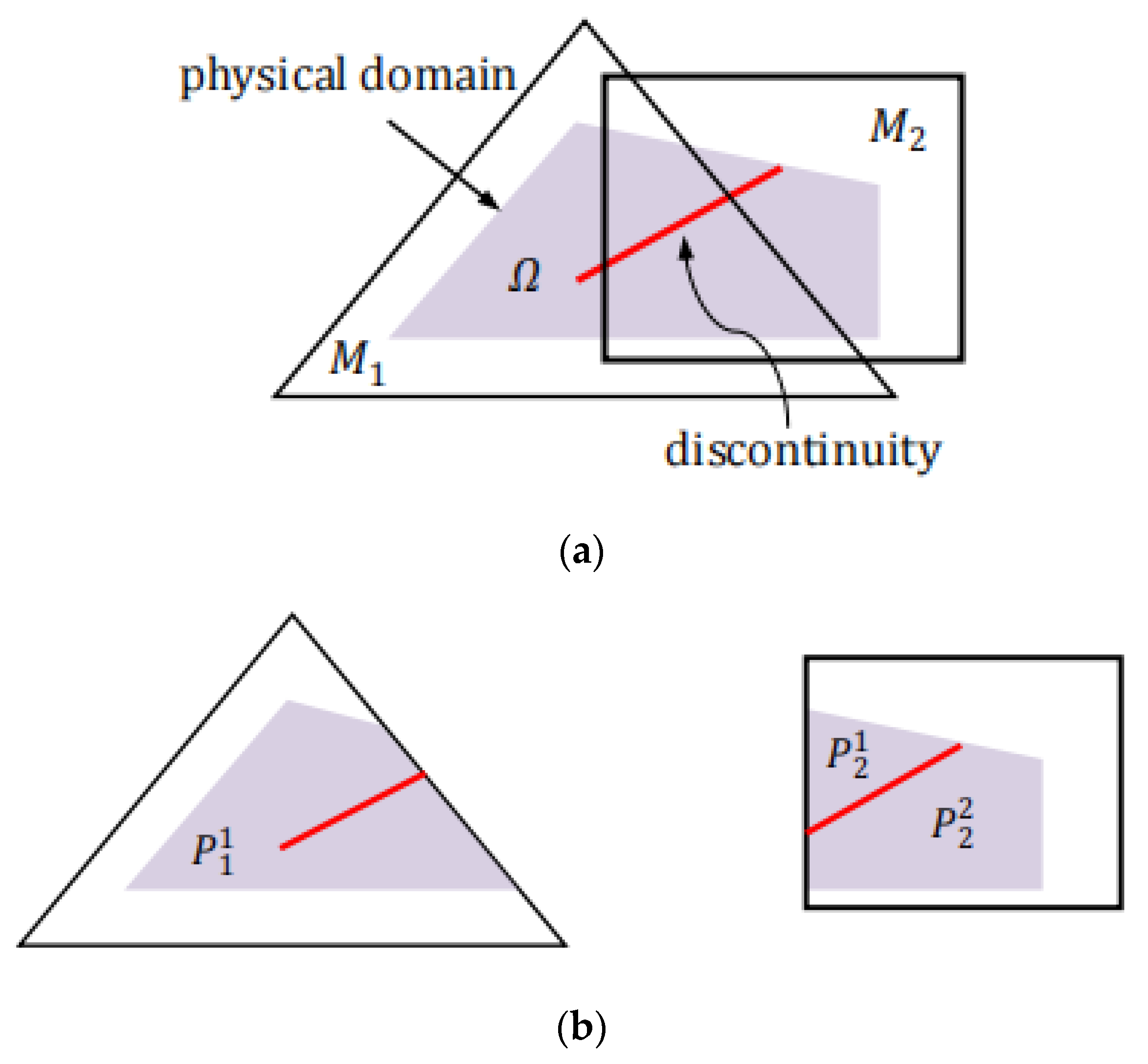
The NMM uses a dual cover system: the mathematical cover (MC) and physical cover (PC). Figure 1 illustrates an example of a physical domain with an internal discontinuity overlapped by two MCs denoted by the triangle $M_1$ and rectangle $M_2$, respectively. The MCs are independently constructed and do not need to conform to the domain boundaries and the internal discontinuities (e.g., bedding, crack, joint, interlayer, etc.). The PCs are a sub-set of the MCs obtained from intersections with the physical domain. A manifold element (ME) is generated as the common area of the overlapped PCs. As plotted in Figure 1a, each patch (i.e., triangle and rectangle) is termed as a MC, denoted by M_i (i = 1, 2); external boundary and internal joints or cracks may split one MC into several separate sub-patches, each one within the material domain $\Omega$ is regarded as a PC, which is denoted by $P_i^j$ (I = 1, 2; j = 1, 2). Figure 1b shows that the material domain $\Omega$ is intersected by patch $M_1$ to generate one PC, denoted by $P_1^1$. When internal discontinuities (i.e., cracks or joints) exist, each discontinuity is considered as one special physical domain to form new PCs. When a crack passes through the whole patch within the material domain, two isolated PCs are formed by the crack in $M_2$, and denoted by $P_2^1$ and $P_2^2$, respectively. When the crack cuts MC partially, only one PC is produced within the material domain such as $P_1^1$. The common area of several overlapping PCs is termed as a ME. As can be seen in Figure 1c, five MEs were formed by the overlapping $P_1^1$, $P_2^1$, and $P_2^2$, which can be represented by $E_1\left(P_1^1\right)$, $E_2\left(P_1^1{\displaystyle \cap }{P}_2^1\right)$, $E_3\left(P_1^1{\displaystyle \cap }{P}_2^2\right)$, $E_4\left(P_2^1\right)$, and $E_5\left(P_2^2\right)$, respectively.

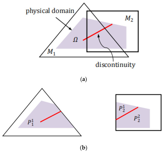
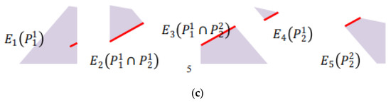
Figure 1. An illustration of the cover system of the NMM: (a) MCs and physical domain; (b) PCs; (c) MEs.

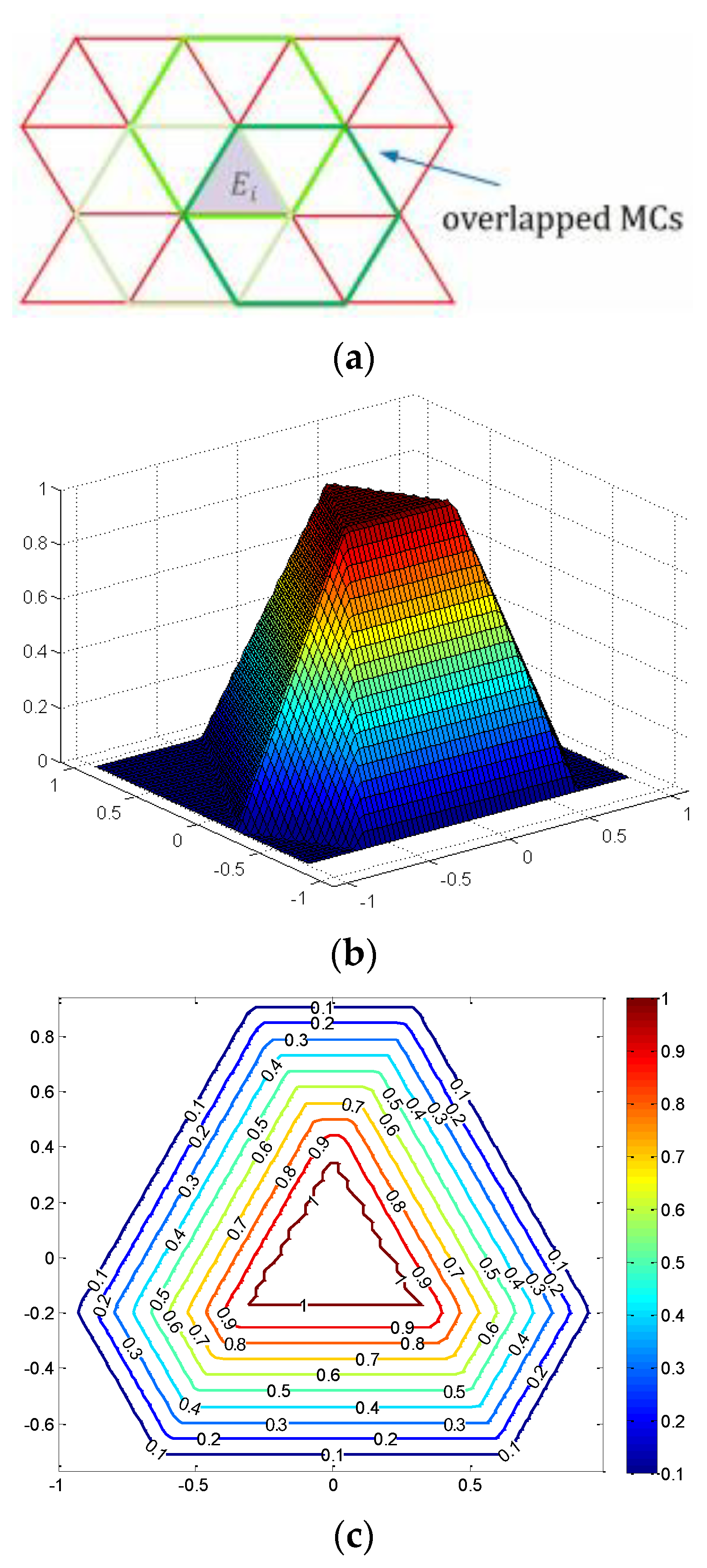
Since the NMM does not require MC sides to coincide with the material boundaries and discontinuities, arbitrary shape MCs can be employed. For convenience, a regularly structured mathematical mesh was employed in the NMM. As seen in Figure 2a, a regular triangular mesh was constructed, in which each MC was formed through six neighboring triangular elements sharing a common node (i.e., nodal star). Each MC had two degrees of freedom (DOFs), which was similar to the node property of the FEM. The mathematical mesh covered the whole physical domain to form a PC system, where the common areas denoted by $E_i$ ($i\in Natural number$) was formed by the neighboring three hexagonal PCs. When the linear triangular element PU function is applied into the cover system, the global displacement function over a ME can be expressed as:

$$U_e\left(x,y\right)={{\displaystyle \sum }}_{i=1}^3{w}_i\left(x,y\right)D_i\left(x,y\right)and\left(x,y\right)\in {\Omega }_e$$

(1)

where $w_i\left(x,y\right)$ is the PU function over the three associated PCs; $D_i\left(x,y\right)={\left\{\begin{array}{cc}{u}_i\left(x,y\right)& v_i\left(x,y\right)\end{array}\right\}}^T$ is the displacement function on the three PCs; and ${\Omega }_e$ is the problem domain covering the MEs. The dual cover system makes the solution suitable to both continuous and discontinuous problems without any re-meshing technique, as conducted in the FEM.

Figure 2. PU of weight functions over the triangular mesh: (a) Manifold element and overlapped MCs; (b) PU function; (c) contour of the PU function.

In the two-dimensional NMM, a PU function $w_i\left(x,y\right)$ is defined on a PC $P_i$ such that

$$\begin{array}{c}{w}_i\left(x,y\right)\ge 0, if \left(x,y\right)\in P_i\\ w_i\left(x,y\right)=0, if \left(x,y\right)\notin P_i\end{array}\}$$

(2)

The PU function is a partition of unity and satisfies

$${{\displaystyle \sum }}_{\left(x, y\right)\in P_j}{w}_j\left(x,y\right)=1$$

(3)

Using the weight function $w_i\left(x,y\right)$, the global displacement function $U\left(x,y\right)$ and $V\left(x,y\right)$ on the whole PC system can be defined based on the following local displacement functions $u_i\left(x,y\right)$ and $v_i\left(x,y\right),$ respectively, as

$$\left\{\begin{array}{c}U\left(x,y\right) \\ V\left(x,y\right) \end{array}\right\}={{\displaystyle \sum }}_{i=1}^n{w}_i\left(x,y\right)\left\{\begin{array}{c}{u}_i\left(x,y\right) \\ v_i\left(x,y\right) \end{array}\right\}$$

(4)

where n is the number of PCs equal to 3 for a 2D problem. When the triangular finite element mesh and a constant cover function are used, the global displacement on each ME can be rewritten as

$$\left\{\begin{array}{c}{U}_e\left(x,y\right) \\ V_e\left(x,y\right) \end{array}\right\}=\left[T_e\left(x,y\right)\right]\left\{D_e\right\}=\left[\begin{array}{ccc}{T}_{e\left(1\right)}\left(x,y\right)& T_{e\left(2\right)}\left(x,y\right)& T_{e\left(3\right)}\left(x,y\right)\end{array}\right]\left\{\begin{array}{c}{D}_{e\left(1\right)}\\ D_{e\left(2\right)}\\ D_{e\left(3\right)}\end{array}\right\}$$

(5)

where $\left[T_{e\left(i\right)}\left(x,y\right)\right]=\left(\begin{array}{cc}{w}_{e\left(i\right)}\left(x,y\right)& 0\\ 0& w_{e\left(i\right)}\left(x,y\right)\end{array}\right)$, $\left\{D_{e\left(i\right)}\right\}=\left\{\begin{array}{c}{u}_{e\left(i\right)}\left(x,y\right)\\ v_{e\left(i\right)}\left(x,y\right)\end{array}\right\}$, i = 1, 2, 3. Thus, the FEM is a special case of the NMM when the cover function is constant and the weight function is the shape function in the FEM.

In this study, we considered a 2-dimensional problem based on regular triangular grids. The finite element shape function of the triangle naturally forms a uniform division (PU) from the mathematical patch, as shown in Figure 2b. As shown in the following case, consider a ME $E_i$ $\left(i\in N\right)$ formed by three associated PCs, three overlapping PCs of PU functions on a regular hexagonal patch, where each PC consists of six equilateral triangle elements, called flat-top PU [33]. The images and profiles of the PU function are shown in Figure 2b,c, respectively. Using the method in [34], we proved that the flat-top PU approximation built by the triangular mesh was linearly independent at the global level.

2.2. Open–Close Iteration Algorithm

In the original NMM computations, when the contact criteria of no-penetration and no-tension could not be satisfied within six iterations in one open–close iteration (OCI), the calculated time step was reduced to one-third of the initial time step, and then the OCI was restarted again. The number of OCIs also depends on the input parameters (e.g., the time step). Larger time steps can lead to more OCIs to achieve contact criteria [10]. High-performance computing enables the NMM to challenge structural dynamic simulations including numerous discontinuous blocks. Nevertheless, the OCIs in NMM met the requirements of non-free and tension-free criteria. The correctness of the contact judgment criterion and the computational cost of the contact requirements at each time step control the entire computational efficiency of the NMM.

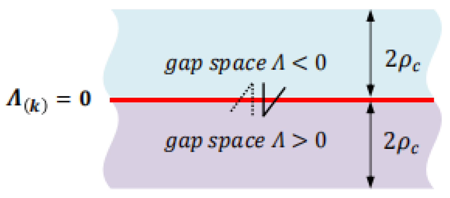
The traditional NMM uses a penalty method with parameter $p$ and gap function of $G=G\left(\Lambda \right)$, where $\Lambda$ is the gap space vector for the detected contact pairs. As plotted in Figure 3, given a contact judgment distance $2{\rho }_c$ to detect the potential contact boundary, where ${\rho }_c=max\left\{\sqrt{{\displaystyle \sum }{u}_l{\left(x,y\right)}^2}\right\},\forall \left(x, y\right)\in B_l, l=1, 2, \cdots , r$; $u_l\left(x, y\right)$ is the global approximation to the block boundary $B_l$; and $r$ is the total number of potential contact boundaries. The contact stiffness $K$ and contact force $F$ can be determined using the penalty method as the form of

$$\{\begin{array}{c} p{G}_{\left(k\right)}{G}_{\left(k\right)}^T⇢K_{\left(k\right)}\\ -p{d}_{\left(k\right)}{G}_{\left(k\right)}⇢F_{\left(k\right)}\end{array}$$

(6)

where $k$ is the number of iterations for the current OCI and $d_{\left(k\right)}$ is the penetration distance at the $k$th iteration. $K_{\left(k\right)}⇢{\stackrel{=}{K}}_{\left(k\right)}$ forms the global stiffness term, and $F_{\left(k\right)}⇢{\stackrel{=}{F}}_{\left(k\right)}$ generates the global force vectors for the equilibrium equation of motion system. The next iterative displacements of $D_{\left(k+1\right)}$ over the iterative number $k$ satisfy the relational expression of

$$D_{\left(k+1\right)}={\overline{K}}_{\left(k\right)}^{-1}{\overline{F}}_{\left(k\right)}$$

(7)

where ${\overline{K}}_{\left(k\right)}={\overline{K}}_{\left(k-1\right)}+{\Lambda }_{\left(k\right)}{\stackrel{=}{K}}_{\left(k\right)}$, and ${\overline{F}}_{\left(k\right)}={\overline{F}}_{\left(k-1\right)}+{\Lambda }_{\left(k\right)}{\stackrel{=}{F}}_{\left(k\right)}$ for the initiation of ${\overline{K}}_{\left(0\right)}={\stackrel{=}{K}}_{\left(0\right)}$ and ${\overline{F}}_{\left(0\right)}={\stackrel{=}{F}}_{\left(0\right)}$. Within the number of iterations of $k\le 6$, the final condition for OCI convergence at ${\Lambda }_{\left(k\right)}=0$ A is

$$\frac{\parallel d_{\left(k\right)}\parallel }{\parallel d_{\left(0\right)}\parallel }<\delta$$

(8)

where $d_{\left(0\right)}$ is the initial search penetration distance of the contact pair, and $\delta$ with the set tolerance value between 10⁻⁴ and 10⁻⁶. Therefore, an appropriate contact stiffness p or time step is required to prevent poor contact penetration.

Figure 3. Description of gap space vector $\Lambda$ for the contact pair.

3. The G-α Time Integration

The motion equation of linear dynamic problems can be expressed in the following under the consideration of the initial conditions:

$$\{\begin{array}{c}M\ddot{d}\left(t\right)+C\dot{d}\left(t\right)+Kd\left(t\right)=F\left(t\right)\\ d\left(0\right)=d_0, \dot{d}\left(0\right)={\dot{d}}_0\end{array}$$

(9)

where $M$, $C$, and $K$ are the mass, damping, and stiffness matrices, respectively; $F\left(t\right)$ is the vector of applied load; $\ddot{d}\left(t\right)$, $\dot{d}\left(t\right),$ and $d\left(t\right)$ are the vectors of acceleration, velocity, and displacement at time $t$, respectively; and $d_0$ and ${\stackrel{·}{d}}_0$ are the vectors of the initial displacements and velocities, respectively. The exact solution of Equation (9) can be replaced by the approximations of ${\ddot{u}}_n$, ${\dot{u}}_n$, and $u_n$ at the time $t_n=n\Delta t$, where $n$ is the nth time step, and $\Delta t$ is the time increment, respectively. Then, ${\ddot{u}}_{n+1}$, ${\dot{u}}_{n+1}$ and $u_{n+1}$ are approximated using the Taylor series as follows:

$${\ddot{u}}_{n+1}={\ddot{u}}_n+\Delta \ddot{u}$$

(10a)

$${\dot{u}}_{n+1}={\dot{u}}_n+{{\displaystyle \int }}_{t_n}^{t_{n+1}}\ddot{u}(\daleth )d\daleth$$

(10b)

$$u_{n+1}=u_n+\Delta t{\dot{u}}_n+{{\displaystyle \int }}_{t_n}^{t_{n+1}}\ddot{u}(\daleth )\left(t_{n+1}-\daleth \right)d\daleth$$

(10c)

where $\Delta \ddot{u}$ is the increment of the acceleration. Substituting Equations (10a), (10b) and (10c) into Equation (9), the discrete form of the equation can be re-expressed as follows:

$$M{\ddot{u}}_{n+1}+C{\dot{u}}_{n+1}+K{u}_{n+1}=F_{n+1}$$

(11)

where $F_{n+1}$ denotes the force vector at time $t_{n+1}=\left(n+1\right)\Delta t$.

In the traditional NMM, an implicit Newmark time integration is conducted by minimizing the potential energy with parameters $\beta =1/2, \gamma =1$. Thus, substituting the parameters into Equation (11), the equation of motion is rewritten as

$$\left[K+\frac{2M}{{\left(\Delta t\right)}^2}\right]\Delta u=F_{n+1}+\frac{2M}{\Delta t}{\dot{u}}_n$$

(12)

where $\Delta u=\left(u_{n+1}-u_n\right)$ is the displacement increment from the time step $t_n$ to $\left(t_n+\Delta t\right)$. The mass matrix of $M$ and stiffness matrix of $K$ inherits the properties of symmetry and sparsity similar to the FEM formula. Since the implicit algorithm is required to assemble the global stiffness matrix and solve the coupled system equation, the computational cost is raised, especially when the OCIs of contact treatment are applied in the NMM code. Moreover, an appropriate ∆t is determined under the requirement of numerical damping. For the best results from stability and numerical dissipation point of view, a time step $\Delta t$ is considered as [35]:

$$\Delta t\le \left(\frac{4}{{\omega }_{max}^e}\right)$$

(13)

where ${\omega }_{max}^e$ is the element maximum angle frequency of system.

The G-α method in the present study is an unconditionally stable, second-order accuracy time integration, which possesses an optimal combination of high-frequency and low-frequency dissipation. Formula of the G-$\mathsf{\alpha }$ method resorting to the Newmark method frame can be expressed as follows:

$$M{\ddot{u}}_{n+1-{\alpha }_m}+C{\dot{u}}_{n+1-{\alpha }_f}+K{u}_{n+1-{\alpha }_f}=F_{n+1-{\alpha }_f}$$

(14)

where

$$u_{n+1-{\alpha }_f}=\left(1-{\alpha }_f\right)u_{n+1}+{\alpha }_f{u}_n$$

(15a)

$${\dot{u}}_{n+1-{\alpha }_f}=\left(1-{\alpha }_f\right){\dot{u}}_{n+1}+{\alpha }_f{\dot{u}}_n$$

(15b)

$${\ddot{u}}_{n+1-{\alpha }_m}=\left(1-{\alpha }_m\right){\ddot{u}}_{n+1}+{\alpha }_m{\ddot{u}}_n$$

(15c)

$$F_{n+1-{\alpha }_f}=\left(1-{\alpha }_f\right)F_{n+1}+{\alpha }_f{F}_n$$

(15d)

where $n\in \left\{0, 1, \cdots ,N-1\right\}$; $N$ is the total number of time step; coefficients ${\alpha }_m$ and ${\mathsf{\alpha }}_f$ are the two control parameters of the algorithm; and ${\ddot{u}}_n$ and ${\ddot{u}}_{n+1}$, ${\dot{u}}_n$ and ${\dot{u}}_{n+1}$, $u_n$ and $u_{n+1}$, are the accelerations, velocities, and displacements at time $t_n$ and $t_{n+1}$, respectively. These approximations satisfy the Newmark method to be expressed as

$$\{\begin{array}{c} u_{n+1}=u_n+\theta ·\Delta t·{\dot{u}}_n+\left(\frac{1}{2}-\beta \right)\Delta t^2·{\ddot{u}}_n+\beta \Delta t^2·{\ddot{u}}_{n+1}\\ {\dot{u}}_{n+1}=\theta ·{\dot{u}}_n+\left(1-\gamma \right)\Delta t·{\ddot{u}}_n+\gamma \Delta t·{\ddot{u}}_{n+1} \end{array}$$

(16)

where $\beta$ and $\gamma$ are the two parameters determining the algorithm property and $\theta$ is the kinetic damping to discount velocity and satisfies $\theta \in \left[0, 1\right]$. Accordingly, the global equilibrium equation can be obtained when $\theta$ equals to 1, and the more details of the derivation can be referred to in Appendix A.

The G-α method is of second-order accuracy for

$$\gamma =\frac{1}{2}-{\alpha }_m+{\alpha }_f,$$

(17)

which achieves optimal high frequency dissipation with a minimal low frequency effect to damp spurious oscillations when the following conditions hold:

$${\alpha }_f=\frac{{\alpha }_m+1}{3} \mathrm{and} \beta =\frac{1}{4}{\left(1-{\alpha }_m+{\alpha }_f\right)}^2$$

(18)

With an appropriate choice of parameters of $\beta$ and $\gamma$, the G-α method simplifies to the HHT-α method [4] in the case of ${\alpha }_m=0$ (i.e., G-${\mathsf{\alpha }}_1$ hereafter), the WBZ-α method [5] in the case of ${\alpha }_f=0$ (i.e., G-${\mathsf{\alpha }}_2$ hereafter), and the Newmark family method [2] when ${\alpha }_m={\alpha }_f=0$. The original NMM code adopts the Newmark method with ${\alpha }_m={\alpha }_f=0$ and $\gamma =2\beta =1$, which can be assumed as a special simplified case of the G-α method.

3.1. Stability Analysis of the G-α Method

For a single degree of freedom (SDOF) system, the motion equation can be represented by

$${\ddot{u}}_{n+1-{\alpha }_m}+2\zeta \omega {\dot{u}}_{n+1-{\alpha }_f}+{\omega }^2{u}_{n+1-{\alpha }_f}=q$$

(19)

where $\zeta =C/\left(2\sqrt{KM}\right)$ is the damping ratio; $\omega =\sqrt{K/M}$ is the natural frequency; and $q$ represents the mass loading.

The G-α algorithm described in Equation (19) can be investigated using the analytical method [1,8]. For this purpose, the algorithm can be converted to another form:

$$\left(\begin{array}{c}{u}_{n+1}\\ \Delta t{\dot{u}}_{n+1}\\ \Delta t^2{\ddot{u}}_{n+1}\end{array}\right)=A\left(\begin{array}{c}{u}_n\\ \Delta t{\dot{u}}_n\\ \Delta t^2{\ddot{u}}_n\end{array}\right)+L\left(\begin{array}{c}{q}_n\\ q_{n+1}\end{array}\right)$$

(20)

where $A$ is the amplification matrix that determines algorithmic characteristics such as stability, accuracy, and numerical dissipation; $L$ denotes the load operator; and $q_n$ and $q_{n+1}$ are the loading at time $t_n$ and $t_{n+1}$, respectively. The amplification matrix $A$ is obtained by the derivations of Equation (20), expressed as:

$$A=\left[\begin{array}{ccc}1+\beta A_{31}& \theta +\beta A_{32}& \frac{1}{2}-\beta \left(1-A_{33}\right)\\ \gamma A_{31}& \theta +\gamma A_{32}& 1-\gamma \left(1-A_{33}\right)\\ A_{31}& A_{32}& A_{33}\end{array}\right]$$

(21)

with

$$A_{31}=-\frac{{\Omega }^2}{D}$$

(22a)

$$A_{32}=-\frac{\Omega }{D}\left[\left(1-{\alpha }_f\right)\left(\Omega +2\zeta \right)\theta +2{\alpha }_f\zeta \right]$$

(22b)

$$A_{33}=1-\frac{1}{D}\left[1+\left(1-{\alpha }_f\right)\left(2\zeta +\frac{\Omega }{2}\right)\Omega \right]$$

(22c)

$$D=\left(1-{\alpha }_m\right)+2\left(1-{\alpha }_f\right)\zeta \gamma \Omega +\left(1-{\alpha }_f\right)\beta {\Omega }^2$$

(22d)

$$\Omega =\omega \Delta t$$

(22e)

The eigenvalues of $A$ are determined by the characteristic equation of

$$-\det \left(A-\lambda I\right)={\lambda }^3-2A_1{\lambda }^2+A_2\lambda -A_3=0$$

(23)

where

$$A_1=\frac{1}{2}trace\left(A\right)$$

(24a)

$$A_2=\frac{1}{2}\left(trace{\left(A\right)}^2-trace\left(A^2\right)\right)$$

(24b)

$$A_3=\det \left(A\right)$$

(24c)

To measure the accuracy of the time integration, two solutions of the characteristic Equation (23) are considered: two complex conjugate roots (denoted as ${\lambda }_1{}_{}$, ${\lambda }_2$) and one real root (denoted as ${\lambda }_3$), which satisfies the condition of

$${\lambda }_{1, 2}=a\pm bi, \left|{\lambda }_3\right|\le \left|{\lambda }_{1, 2}\right|$$

(25)

Specifically, $a$ and $b$ are the real parts and imaginary parts, $i=\sqrt{-1}$, or the three real roots of ${\lambda }_1$, ${\lambda }_2$, and ${\lambda }_3$.

The spectral radius $\rho \left(A\right)$, the algorithmic damping $\overline{\zeta }$, and the relative period error $E_r$ are commonly used as criteria for the performance of an algorithm in comparisons with single step integration methods [19]. These parameters can be defined as:

$$\rho \left(A\right)=\underset{i=1,2,3}{max}\left|{\lambda }_i\right|=max\left\{\left|{\lambda }_1\right|,\left|{\lambda }_2\right|,\left|{\lambda }_3\right|\right\}$$

(26)

$$\overline{\zeta }=-\frac{ln\left(a^2+b^2\right)}{2\overline{\Omega }}$$

(27)

$$E_r=\frac{\overline{T}-T}{T}=\frac{\Omega }{\overline{\Omega }}-1$$

(28)

where $\overline{\Omega }=\arctan \left(b/a\right)=\overline{\omega }\Delta t$, $T=2\pi /\omega$, $\overline{T}=2\pi /\overline{\omega }$.

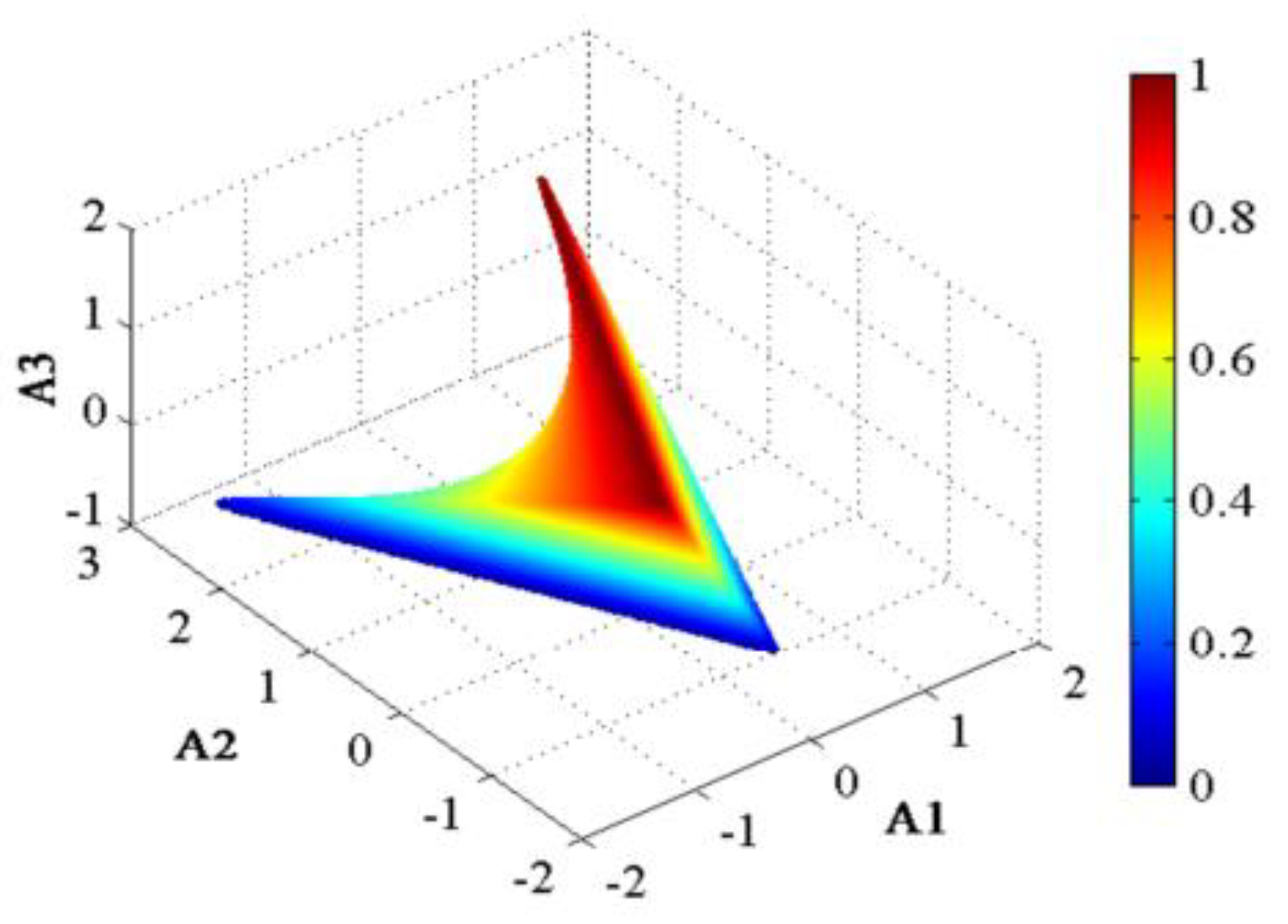
Using the procedure in [8], the stability criterion $\left|{\lambda }_i\right|\le 1$, $i=1, 2, 3$, is satisfied if the following five conditions are constructed (i.e., space of stability in Figure 4):

$$1-2A_1+A_2-A_3\ge 0$$

(29a)

$$3-2A_1-A_2+3A_3\ge 0$$

(29b)

$$3+2A_1-A_2-3A_3\ge 0$$

(29c)

$$1+2A_1+A_2+A_3\ge 0$$

(29d)

$$1-A_2+A_3\left(2A_1-A_3\right)\ge 0$$

(29e)

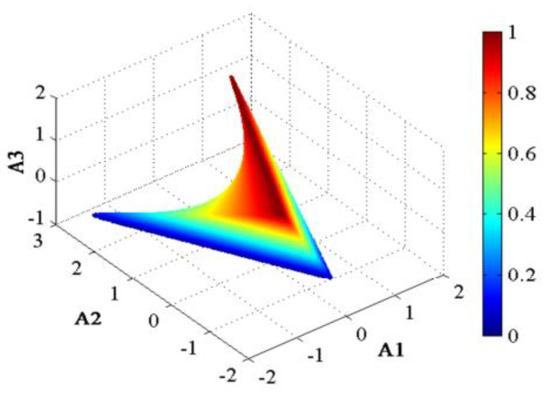
Figure 4. Space of stability in the $A_1{A}_2{A}_3$ coordinate system.

Suppose that $\theta ϵ\left[0, 1\right]$ and $2\beta \ge \gamma \ge \frac{1}{2}$, the above inequalities (i.e., in Equation (29a–e)) all satisfy the requirement of unconditional stability of the G-α algorithm. Therefore, the G-α method is unconditionally stable when the parameters of $\beta =0.3025$ and $\gamma =0.6$; since as described in [19], the NMK-α method used in the original NMM is unconditionally stable with the parameters of $\beta =0.5$ and $\gamma =1$. Furthermore, if $2\beta <\gamma$ and $\gamma \ge \frac{1}{2}$ are both satisfied, the algorithm is conditionally stable. Under this condition, $\Omega \le {\Omega }_{crit}$ must be satisfied in the requirement of $\rho \left(A\right)\le 1$, where ${\Omega }_{crit}$ is the critical sampling frequency and can be expressed as:

$${\Omega }_{crit}=\sqrt{\frac{2\left(1+\theta \right)}{\left(1+\theta \right)\left(\frac{1}{2}-2\beta \right)+2\theta \left(\gamma -2\beta \right)}}$$

(30)

In the present study, the G-${\mathsf{\alpha }}_0$ method (e.g., see Table 1), combined with the G-${\mathsf{\alpha }}_1$ and G-${\mathsf{\alpha }}_2$ methods and the Newmark method of $\gamma =2 \beta =1$ (i.e., denoted as NMK-α), was employed to investigate the algorithm’s performance by the NMM code; more details of the parameters used in the G-α and NMK-α methods can be referred to in Table 1.

Table 1. Selected parameters for the referred methods.

The Referred Methods	${\mathit{\alpha }}_{\mathit{m}}$	${\mathit{\alpha }}_{\mathit{f}}$	$\mathit{\beta }$	$\mathit{\gamma }$
G-${\alpha }_1$	0	1	0.3025	0.6
G-${\alpha }_2$	−0.1	0	0.3025	0.6
G-${\alpha }_0$	0.35	05	0.3025	0.6
NMK-α	0	0	0.5	1.0

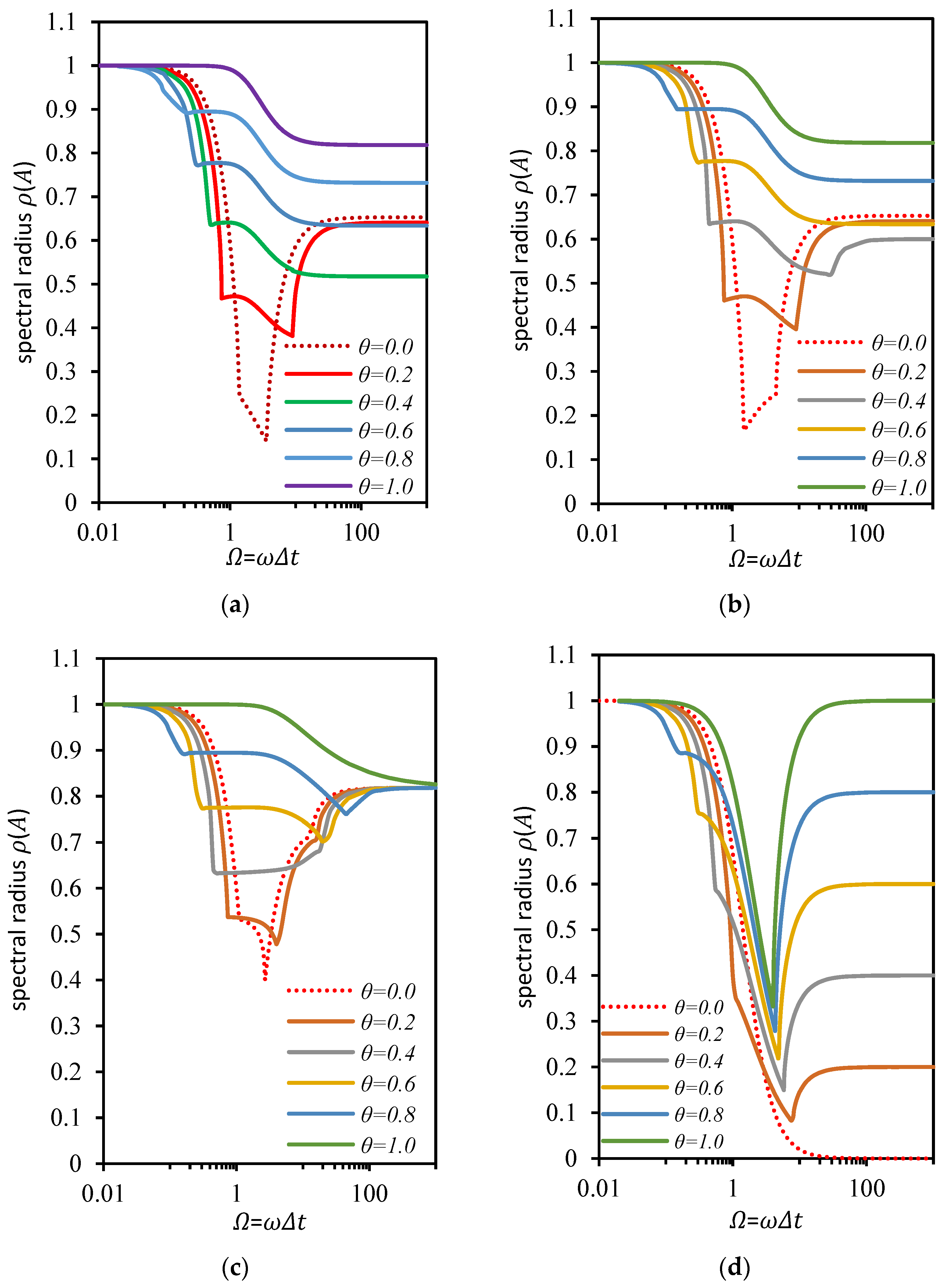
As can be seen in Figure 5, when different values of kinetic damping $\theta$ are employed (i.e., $\theta$ = 0, 0.2, 0.4, 0.6, 0.8, 1), the spectral radius $\rho \left(A\right)$ of the referred algorithms can be calculated as presented in Table 2:

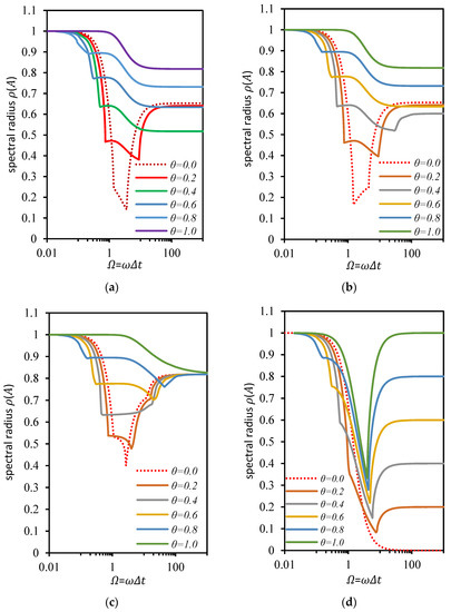
Figure 5. Spectral radius of the algorithms with different values of $\theta$: (a) G-${\mathsf{\alpha }}_1$ method; (b) G-${\mathsf{\alpha }}_2$ method; (c) G-${\mathsf{\alpha }}_0$ method; (d) NMK-α method.

Table 2. Spectral radius $\rho \left(A\right)$ calculated by the referred algorithms.

The Methods	$\mathit{\theta } = 0$	$\mathit{\theta } = 1, \mathit{\Omega }\to \mathit{\infty }$
G-α1	$\Omega \to 3, \rho \left(A\right)\to 0.1617$  $\Omega \to \infty , \rho \left(A\right)\to 0.6338$	$\rho \left(A\right)\to 0.8182$
G-α2	$\Omega \to 1.5, \rho \left(A\right)\to 0.1667$  $\Omega \to \infty , \rho \left(A\right)\to 0.6338$	$\rho \left(A\right)\to 0.8182$
G-α0	$\Omega \to 2.67, \rho \left(A\right)\to 0.3667$  $\Omega \to \infty , \rho \left(A\right)\to 0.8182$	$\rho \left(A\right)\to 0.8182$
NMK-α	$\Omega \to 100, \rho \left(A\right)\to 0$	$\rho \left(A\right)\to 1$

It can be found that the G-${\mathsf{\alpha }}_0$ method possessed similar numerical stability and dissipation to the G-${\mathsf{\alpha }}_1$ and G-${\mathsf{\alpha }}_2$ methods when the same parameters of $\beta$ and $\gamma$ were applied. On the other hand, when $\theta =0$ was used in the NMK-α method, $\rho \left(A\right)\to 0$ could be obtained and the maximum algorithm damping $\overline{\zeta }$ was considered to achieve the fasted convergence velocity, but the numerical accuracy could not be guaranteed. In terms of the period for optimization of the above-mentioned time integration schemes, the G-α method possessed more inbuilt advantage than that of the NMK-α method. Furthermore, the value of ${\Omega }_{\mathrm{bif}}=4$ was also computed in Figure 5d when the NMK-α method was applied to obtain the highest convergences efficiency, where ${\Omega }_{\mathrm{bif}}$ is the bifurcate sampling frequency.

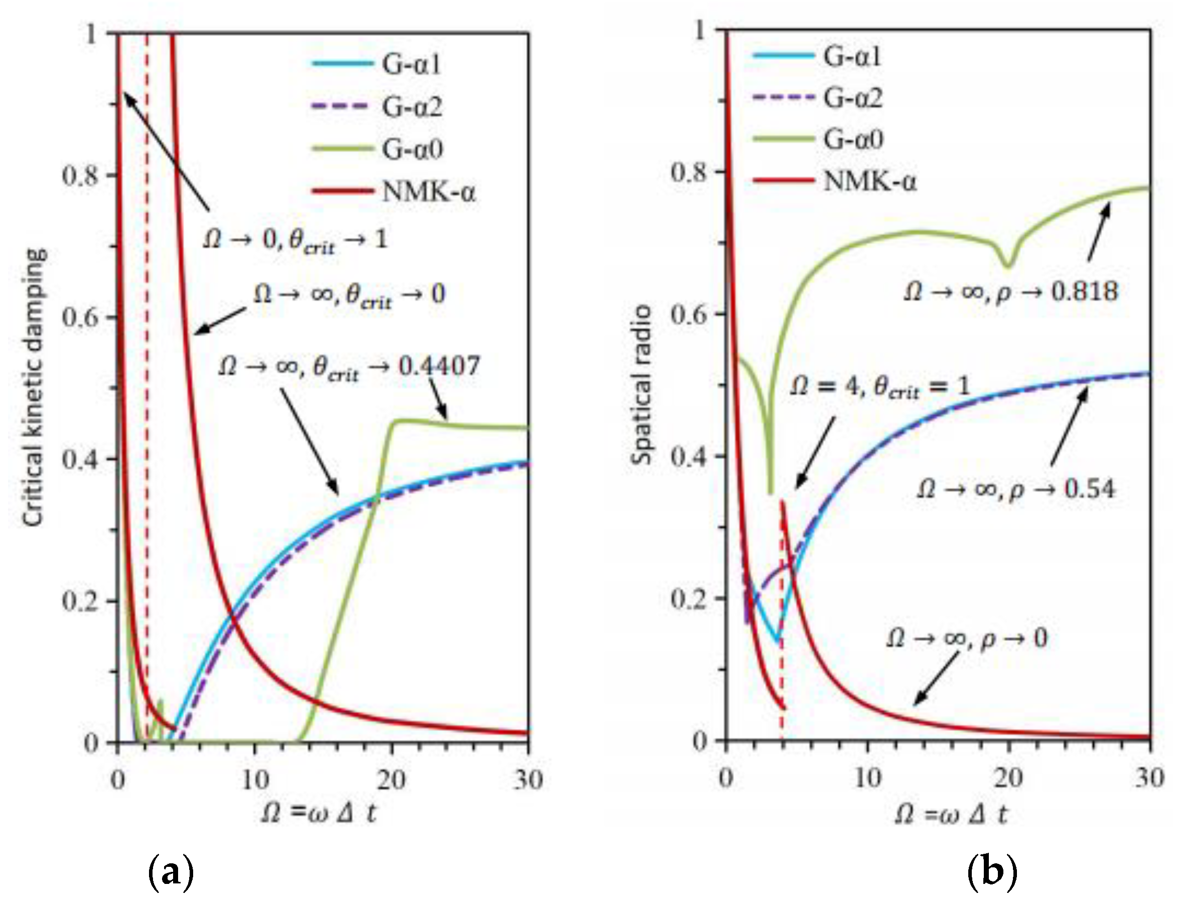
To avoid the decay and saw tooth pattern oscillation, the solution of $u_n={{\displaystyle \sum }}_{i=1}^3{c}_i{\lambda }_i^n$ must satisfy the conditions of $\left|{\lambda }_2\right|>\left|{\lambda }_1\right|>\left|{\lambda }_3\right|$ and ${\lambda }_2<0$. Moreover, $\Omega <{\Omega }_{bif}$ or $\theta >{\theta }_{crit}$ is hold to satisfy the stability condition, where ${\theta }_{crit}$ is called critical kinetic damping. If the value of $\Omega$ is too large or $\theta$ is minor, oscillation will occur, the contact and deformation will also be distorted when the time integration of the G-${\alpha }_0$ method is employed into the computations. At this case, more time steps are required to achieve the solution and OCI convergence. Therefore, if $\Omega ={\Omega }_{bif}$ or $\theta ={\theta }_{crit}$ is adopted, the convergence velocity is the fastest and computational efficiency is the highest. As plotted in Figure 6a, the critical kinetic damping ${\theta }_{crit}$ of the G-${\mathsf{\alpha }}_1$ method, the G-${\mathsf{\alpha }}_2$ method and the G-${\alpha }_0$ method approach to 0.4407 when $\Omega \to \infty$. On the other hand, the NMK-α is different since bifurcation condition has a significant effect on the solution. ${\theta }_{crit}$ satisfies the expression of $\Omega \to 0, {\theta }_{crit}\to 1$ when $\Omega \in [0, {\Omega }_{bif})$, $\Omega \to \infty , {\theta }_{crit}\to 0$ has been achieved at the case of $\Omega \in [{\Omega }_{bif}, \infty )$, where the value of ${\Omega }_{bif}$ is equal to 4. Obviously, it is more complicated to determine time step Δt by ${\Omega }_{bif}$ than cases that considering viscous damping in the NMK-α method, $\Delta t={\Omega }_{bif}/\omega$ normally is larger than the used in practical discontinuous deformation simulations. Thus, the critical kinetic damping ${\theta }_{crit}$ is more preferred than ${\Omega }_{bif}$ in the actual computations. Figure 6b shows the spectral radius $\rho$ by the ${\theta }_{crit}$ when the different methods are considered. Both the G-${\mathsf{\alpha }}_1$ method and the G-${\mathsf{\alpha }}_2$ method possess the same spherical radius $\rho \to 0.54$ at the cases of $\Omega \to \infty , {\theta }_{crit}\to 0.4407$, but the G-${\mathsf{\alpha }}_0$ method is different, which satisfies the condition of $\Omega \to \infty , \rho \to 0.818$ when the same ${\theta }_{crit}$ is selected. For the NMK-α method, when ${\Omega }_{bif}=4$ is taken into account, ${\theta }_{crit}=1$ and $\rho =0.333$ can be only determined by the amplification matrix of A; $\Omega \to \infty , \rho \to 0$ and $\Omega \to 0, \rho \to 1$ are also obtained when different ${\theta }_{crit}$ values are chosen. It is also found that the NMK-α method achieves the maximum ${\theta }_{crit}$ comparing with the other three methods, and minimum spectral radius $\rho$ to attain the fastest convergence of the solution.

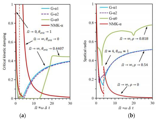
Figure 6. Critical kinetic damping ${\theta }_{crit}$ of the referred methods: (a) ${\theta }_{crit}$ by the sampling frequency $\Omega$; (b) spectral radius by the ${\theta }_{crit}$.

3.2. Accuracy of the G-α Method

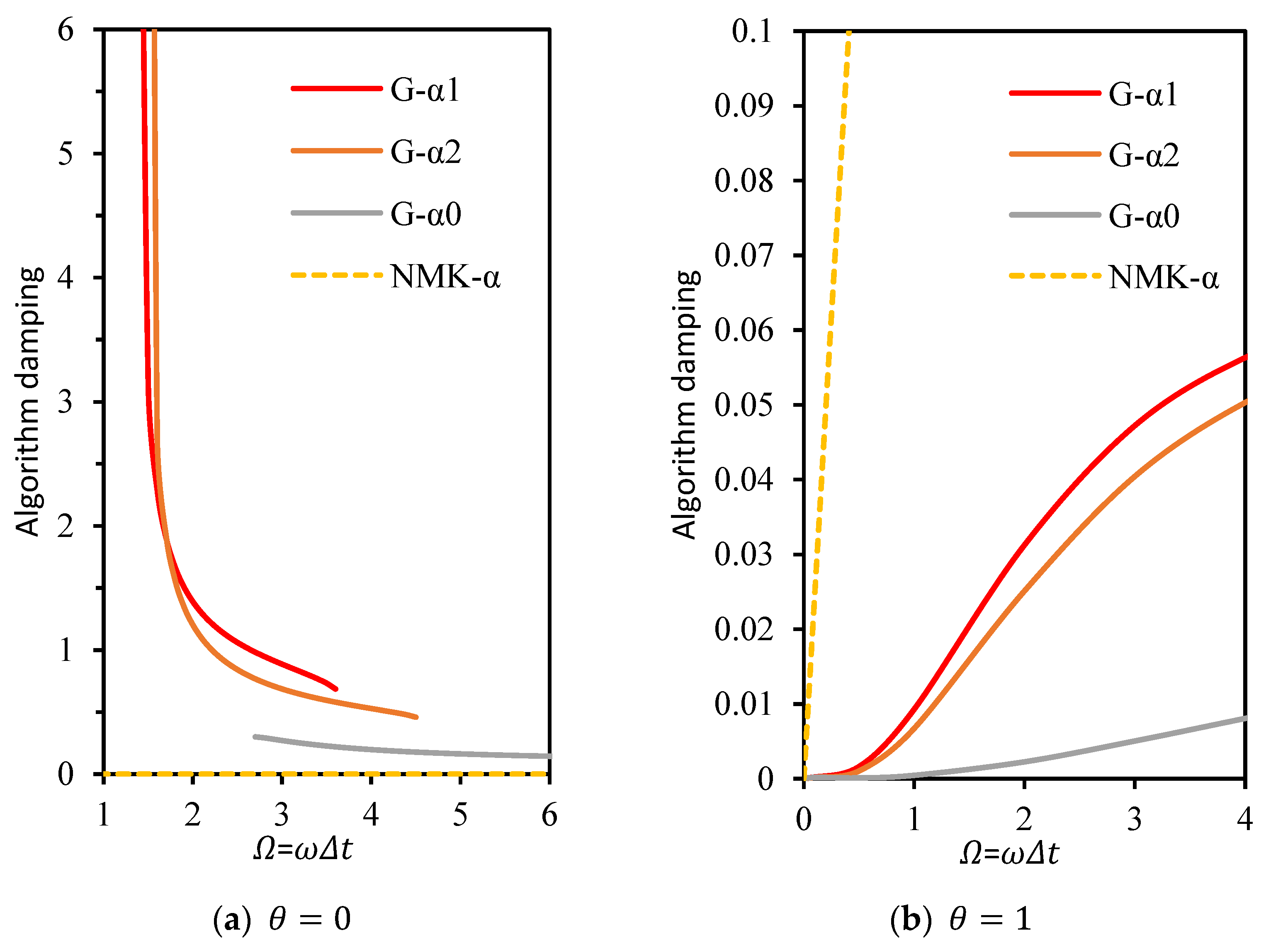
Generally, parameters of algorithmic damping ratio $\overline{\zeta }$ and relative period error $E_r$ are used to measure the numerical dissipation and dispersion of the time integration scheme. In particular, the values of $\overline{\zeta }$ in the cases of $\theta =0$ and $\theta =1$ were plotted in Figure 7 to evaluate the G-α method algorithm accuracy. When $\theta =0$ was considered, the NMK-α method obtained $\overline{\zeta }=0$; the G-α method possessing positive $\overline{\zeta }$ implies that the computed result is convergence. $\overline{\zeta }=0$ means that no numerical dissipation exists by the algorithm, and that spurious oscillations will occur in the computations. When $\theta =1$ was suggested, the NMK-α method possessed the maximum $\overline{\zeta }$ so that the numerical solution approached an exact solution. The G-${\mathsf{\alpha }}_1$ method and the G-${\mathsf{\alpha }}_2$ method had higher $\overline{\zeta }$ than that of the G-${\mathsf{\alpha }}_0$ method in both cases. Thus, it can be concluded that when ${\theta }_{crit}$ is employed, the optimized values of $\overline{\zeta }$ can be observed to control the numerical accuracy of the G-α method.

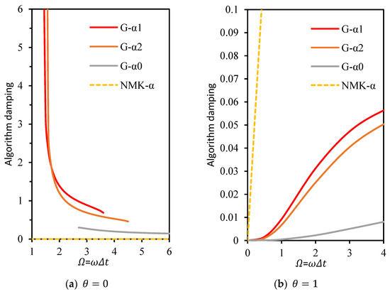
Figure 7. Algorithm damping $\overline{\zeta }$ of the referred methods: (a) $\theta =0$ by the sampling frequency $\Omega$; (b) $\theta =1$ by the sampling frequency $\Omega$.

4. Numerical Examples

To present the performance of the G-α method using the NMM, the aforementioned G-${\mathsf{\alpha }}_0$, G-${\mathsf{\alpha }}_1$, G-${\mathsf{\alpha }}_2$, and NMK-α methods were considered to calibrate the G-α method first, in which one transient dynamical response problem of an elastic bar was simulated. Then, a two-layer system of rock beam deflection was computed to validate the proposed G-α method. Finally, the mechanical behavior of dynamical tunneling was studied using the proposed G-α method to further explore the computational accuracy and efficiency of the proposed algorithm.

4.1. Transient Response of the Elastic Bar

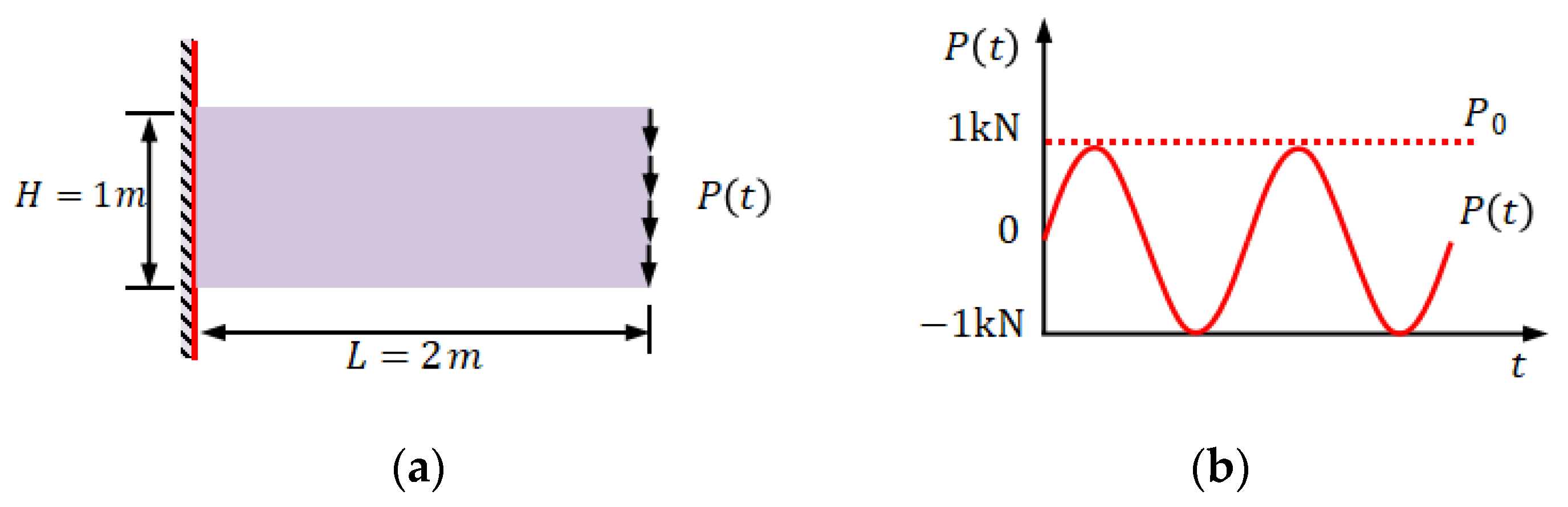
To evaluate the accuracy of the proposed G-α method using the NMM, the transient response of an elastic rock bar was computed. As shown in Figure 8a, a 1.0 m × 2.0 m elastic bar bonded at the left end, and a harmonic function at the right end was applied, which represents the sine function form of $P\left(t\right)=P_{0}sin {\omega }_{0}t$, as shown in Figure 8b, where $P_0=1.0 \mathrm{kN}$, ${\omega }_0=27.7 \mathrm{rad}/\mathrm{s}$. The input physical parameters in the simulations were: Young’s modulus $\mathrm{E}=4.0\times {10}^4$ Pa, Poisson’s ratio 0.25, and the unit mass 1000 kg/m³.

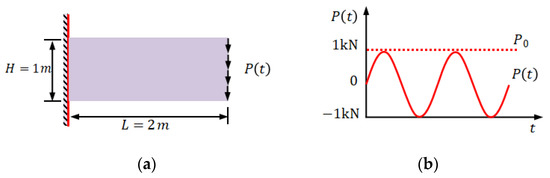
Figure 8. Descriptions of an elastic bar problem: (a) geometry of the elastic bar; (b) applied harmonic function loading.

The theoretical solution of deformation $u\left(t\right)$ to the elasticity problem can be expressed as follows [36]:

$$u\left(t\right)=\frac{P_0\eta }{K}\left[\frac{\delta }{\sqrt{1-{\zeta }^2}}{e}^{-\zeta \omega t}sin\left({\omega }_{D}t+\vartheta \right)+sin\left({\omega }_{0}t-\psi \right)\right]$$

(31)

where $\eta ={\left[{\left(1-{\alpha }^2\right)}^2+4{\zeta }^2{\alpha }^2\right]}^{-\frac{1}{2}}$ is the dynamic magnification factor; $\delta$ is the end deflection under unit loading and satisfies expression of $\delta =L^3/3EI$; and $\psi$ and $\vartheta$ are the two angle phases, which satisfies

$$\{\begin{array}{l}\psi =arctan\frac{2\zeta \alpha }{\left(1-{\alpha }^2\right)}\\ \vartheta =arctan\frac{2\zeta \sqrt{1-{\zeta }^2}}{2{\zeta }^2+{\alpha }^2-1}\end{array}$$

(32)

where $\alpha ={\omega }_0/\omega$; $\omega =\sqrt{K^{*}/M^{*}}$ is the natural frequency; ${\omega }_D=\omega \sqrt{1-{\zeta }^2}$ is the damped natural frequency; $\zeta$ is the damping ratio; and the effective mass $M^{*}$ and stiffness $K^{*}$ are expressed as:

$$\{\begin{array}{l}{M}^{*}=\underset{0}{\overset{L}{{\displaystyle \int }}}\rho {\mathsf{\Phi }}^2\left(x\right)dx=\frac{33}{140}\rho L\\ K^{*}=\underset{0}{\overset{L}{{\displaystyle \int }}}EI\left(x\right){\left({\mathsf{\Phi }}^{″}\left(x\right)\right)}^{2}dx=\frac{3EI}{L^3}\end{array}$$

(33)

where $\rho$ is the density of strip; $\mathsf{\Phi }\left(x\right)$ is the mode shape function vector; $EI$ is the bending stiffness vector; $L$ is the length of the strip; and $E$ is the Young’s modulus.

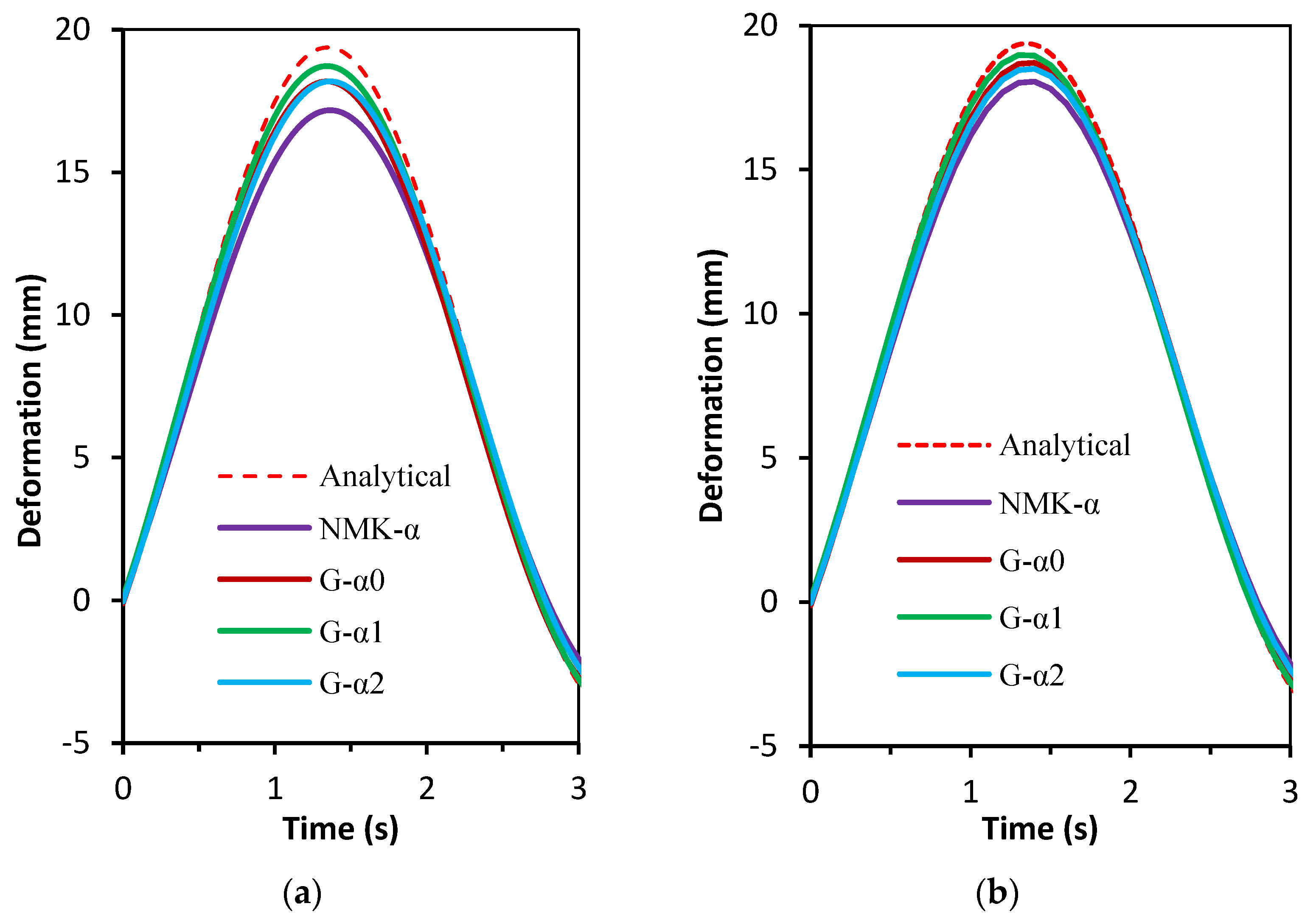
Figure 9 shows the simulations of the elastodynamic problem by the referred time integration schemes with time steps $\Delta t$ = 0.01 s and $\Delta t$ = 0.001 s, respectively. As presented in Figure 9a, the numerical damping was found by both the G-α method and three other methods, and the NMK-α used in the NMM code possessed the strongest damping effect to the simulations. When a smaller time step (i.e., $\Delta t$ = 0.001 s) is employed, as plotted in Figure 9b, an analytical solution can be approached exactly.

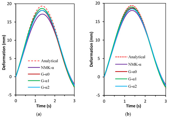
Figure 9. Simulated results of the first crest of deformation: (a) $\Delta t$ = 0.01 s; (b) $\Delta t$ = 0.001 s.

However, when a large time step (i.e., $t$ = 0.01 s) is adopted, stray oscillations occur, and the simulation results are dispersed into the analytical solution.

To verify the computational accuracy to the theoretical solution, the crests’ displacements were calculated using the proposed methods (i.e., the G-${\alpha }_0$, G-${\alpha }_1$, G-${\alpha }_2$, and NMK-α methods), and the simulated results are listed in Table 3. It was found that deformation decreased from the first cases of $\Delta t$ = 0.01 s and $\Delta t$ = 0.001 s. The results from the G-α methods were more accurate than that of the NMK-α method. The G-${\alpha }_0$ method achieved 18.6958 mm at the first crest compared to the NMK-α method of 17.5063 mm when $\Delta t$ = 0.01 s was used. When $\Delta t$ = 0.001 s was used in the simulations, the G-${\alpha }_0$ method approached 18.9768 mm compared to 18.1625 mm of the NMK-α method, while the analytical solution of 19.3378 mm was calculated. The maximum relative errors of the NMK-α method to the analytical solution were 9.4711% and 6.0773% in the different cases.

Table 3. Comparisons of crest deformation using the referred algorithms.

Time Integration	Δt = 0.01 s		Δt = 0.001 s
	1st Crest	2nd Crest	1st Crest	2nd Crest
Analytical solution	19.3378	18.2434	19.3378	18.2434
G-${\alpha }_0$	18.6958	17.6556	18.9768	17.9199
G-${\alpha }_1$	18.1362	17.1547	18.4976	17.4988
G-${\alpha }_2$	18.3562	17.4983	18.7668	17.6761
NMK-α	17.5063	16.6571	18.1625	17.2649
Max. rel. error (%) error (%)	9.4711	8.6952	6.0773	5.3636

4.2. Layered Rock Deflection Simulations

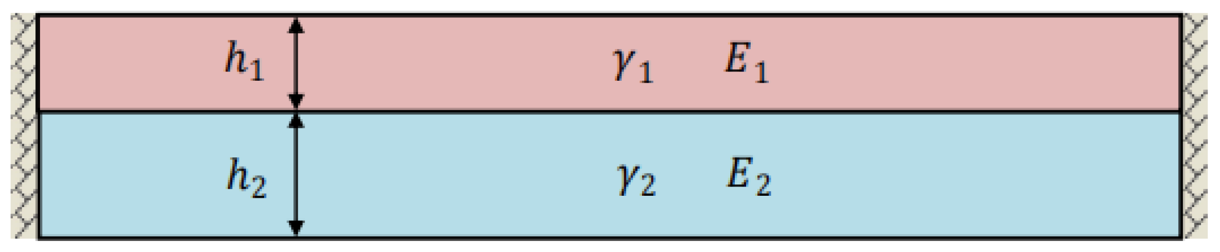
This example analyzed a two-layer system, as shown in Figure 10. The block system was considered as a composite beam with both ends clamped, consisting of a thin beam with Young’s modulus $E_1$, thickness $h_1$, unit weight ${\gamma }_1$, and a thick beam with Young’s modulus $E_2$, thickness $h_2$, and unit weight ${\gamma }_2$. The thin beam was overlaid above the thick beam. Assuming only under gravity, if the deflection of the thin beam is larger than that of the thick beam, the thin beam will push down the bottom thick beam.

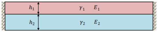
Figure 10. Model of a two-layer system.

An analytical solution for the system can be referred to in [37] when only the self-weigh of the beam was considered, which is expressed as

$$D_{max}=\frac{{\gamma }_e{L}^2}{32E{h}^2}$$

(34)

where $D_{max}$ is the maximum deflection of the beam; ${\gamma }_e$ is the unit weight; and L and h are the length and thickness of the beam, respectively. The derived deflection of the bottom of the system is calculated by assigning it an increased unit weight ${\gamma }_e$, given by:

$${\gamma }_e=\frac{E_2{h}_2^2\left({\gamma }_2{h}_2+{\gamma }_1{h}_1\right)}{E_2{h}_2^3+E_1{h}_1^3}$$

(35)

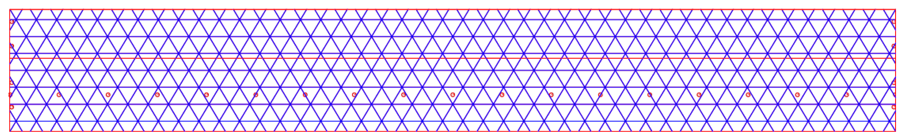
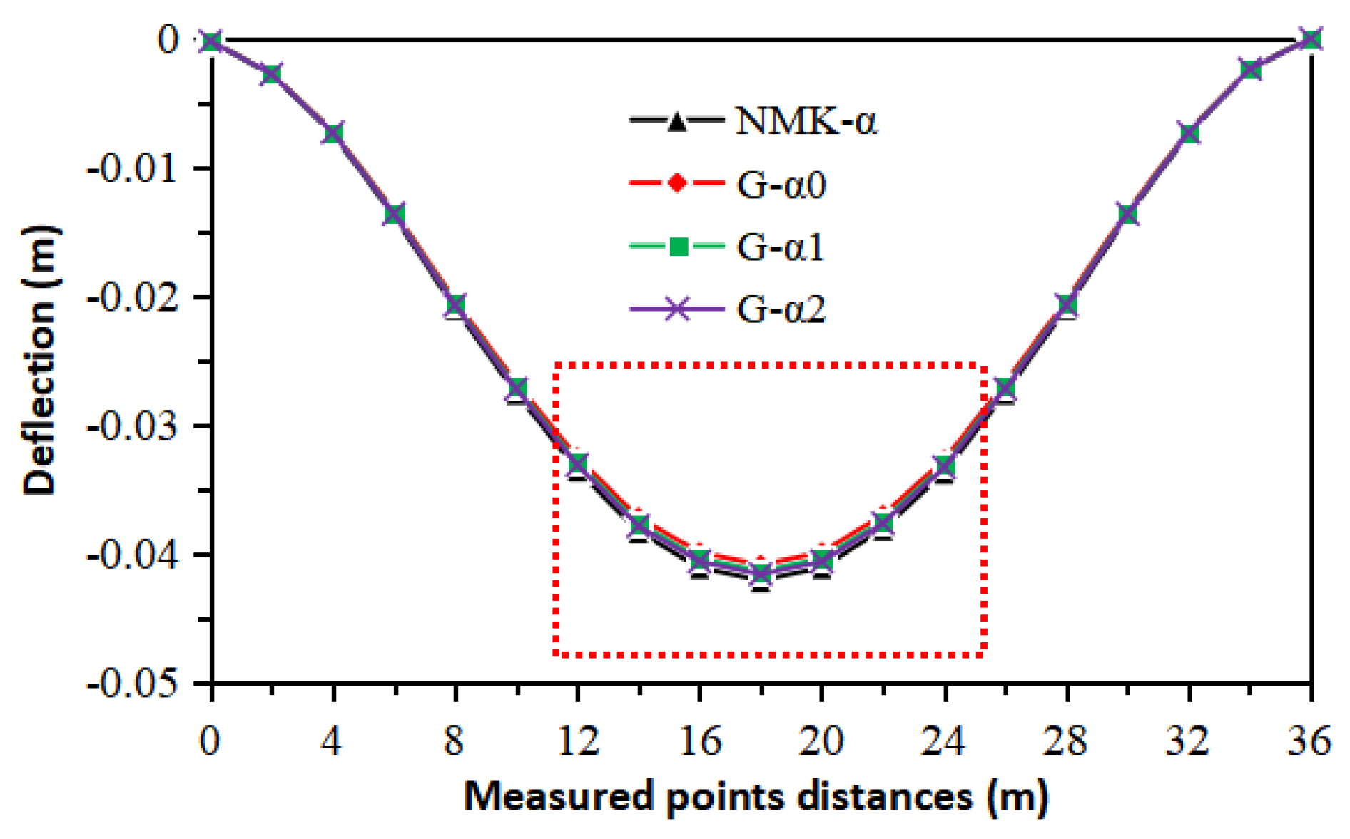
In this simulation, the length of the composite beam was 36 m, and the thicknesses of the upper beam and the lower beam were $h_1$ = 2 m and $h_2$ = 3 m, respectively. Both beams were assumed to have the same material properties: Young’s modulus $E_1=E_2$ = 4.8 GPa, Poisson’s ratio of ${\mathsf{\nu }}_1={\mathsf{\nu }}_2=0.25$, and unit weight ${\gamma }_1={\gamma }_2=$ 25,500 N/m³. Then, the time step size of 0.001 s was used in the modeling. The interface between two layers was assumed to be smooth with zero friction angle and cohesion. In the NMM model, as shown in Figure 11, the composite beam was divided into 1126 manifold elements, and 19 measured points with a spacing of 2 m were prescribed to measure the deflection of the two-layer system.

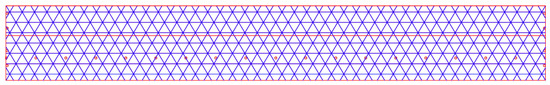
Figure 11. The composite beam model using the NMM.

According to the analytical solution in Goodman [37], it can also be seen that a good agreement was achieved. The maximum deflection of the composite beam was 0.0408 m. After checking the displacements of the measured points from the NMM model, it was found that the maximum deflections of the bottom were both close to the analytical solution with 0.0414 m by the proposed G-${\mathsf{\alpha }}_0$ method and 0.0408 m using the original NMK-α method. The vertical deflections of these measured points from the NMM model were also plotted in Figure 12 against those from the NMM.

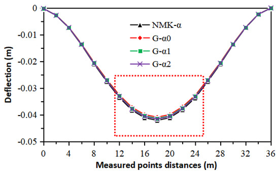
Figure 12. Comparison of the deflection results between the NMK-α and G-α methods.

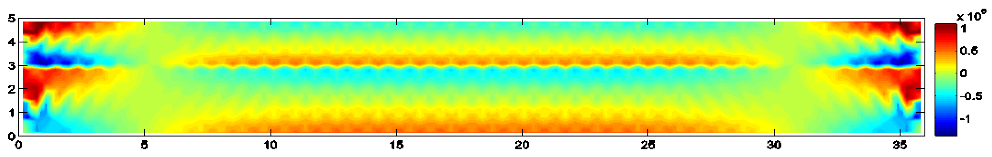
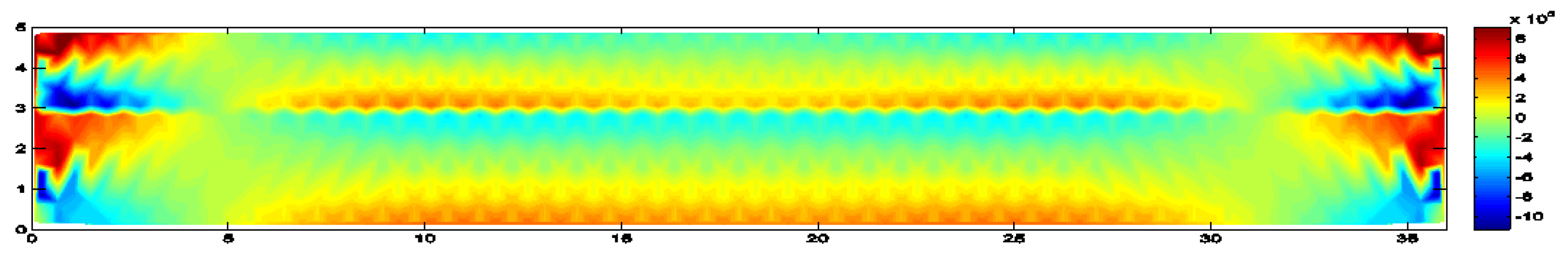
It could also be seen that good agreement was achieved. The ${\sigma }_x$ contour of the lower beam obtained by the G-${\mathsf{\alpha }}_0$ and the NMK-α method are presented in Figure 13 and Figure 14, respectively. In terms of efficiency, the G-${\mathsf{\alpha }}_0$ and the NMK-α methods were employed to analyze the example on the same computer with a processor speed of 4.0 GHz and installed memory of 8 GB. The CPU time was 5.22 and 6.36 min for both methods, respectively. It can be concluded that given the same accuracy, the G-${\mathsf{\alpha }}_0$ method was relatively more efficient than the original NMK-α method by the NMM.

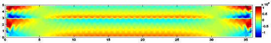
Figure 13. The contour of ${\sigma }_x$ of the lower beam by the G-${\mathsf{\alpha }}_0$ method.

Figure 14. The contour of ${\sigma }_x$ of the lower beam by the NMK-α method.

4.3. Simulation of Behaviors of Blocks on Shaking Table

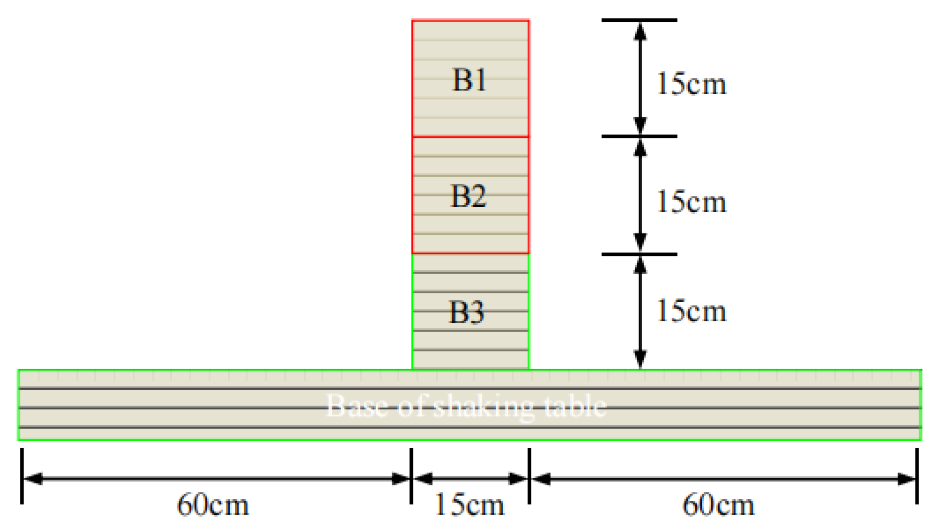
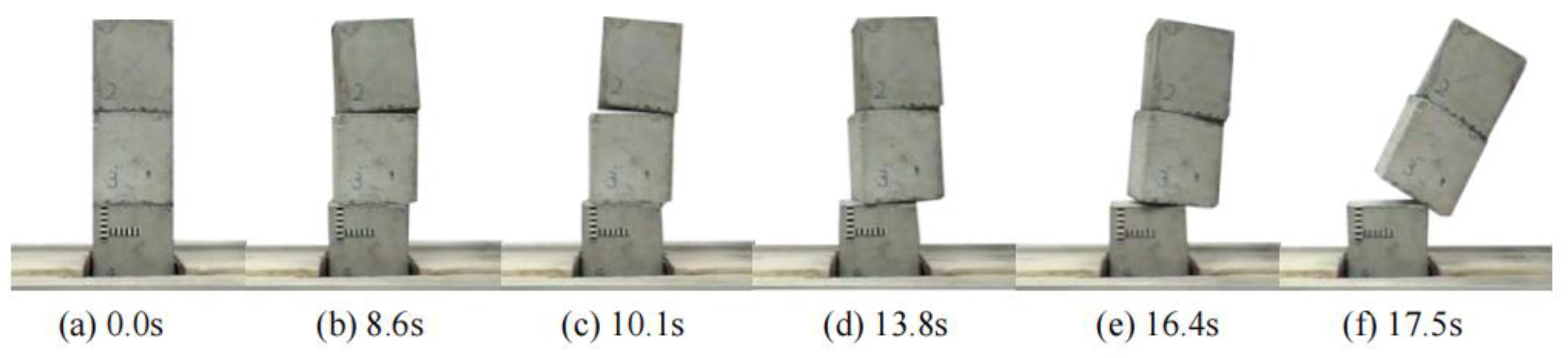
In the simulations, as plotted in Figure 15, an assembled block system consisted of three cubic concrete blocks, the size of each block was 15 cm × 15 cm × 15 cm, and the density was 2200 kg/m³. The numerical model is shown in Figure 16 and the physical properties of block and parameters used in this analysis were: Poisson’s ratio of 0.25, friction angle of 36.4°, Young’s modulus of 14.9 GPa, and contact stiffness of 200 GPa, respectively. Then, the time step size of 0.001 s was applied to both methods and the results of the simulation in the case of a frequency of 5.0 Hz and amplitude of 0.7138 g vibration are shown in Figure 17.

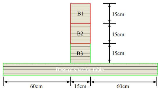
Figure 15. Physical model of the assembled blocks standing on the shaking table.

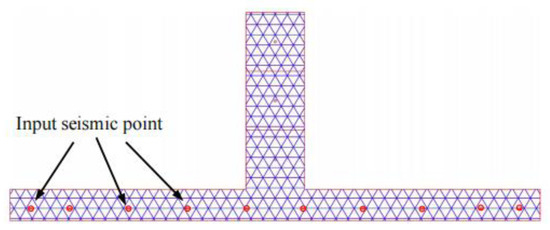
Figure 16. Numerical model of the assembled block system by the NMM.

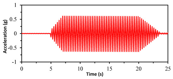
Figure 17. Input horizontal seismic acceleration.

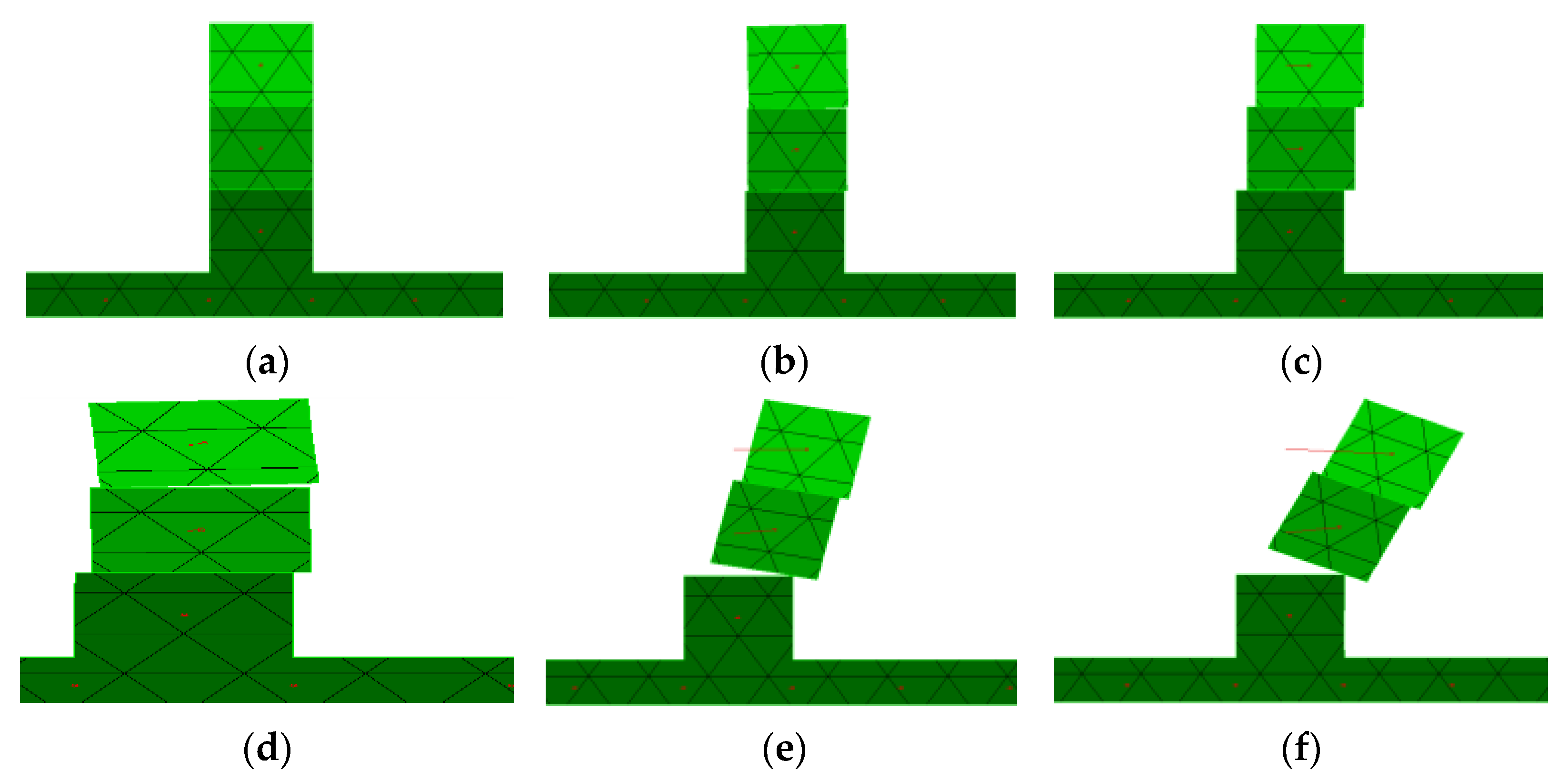
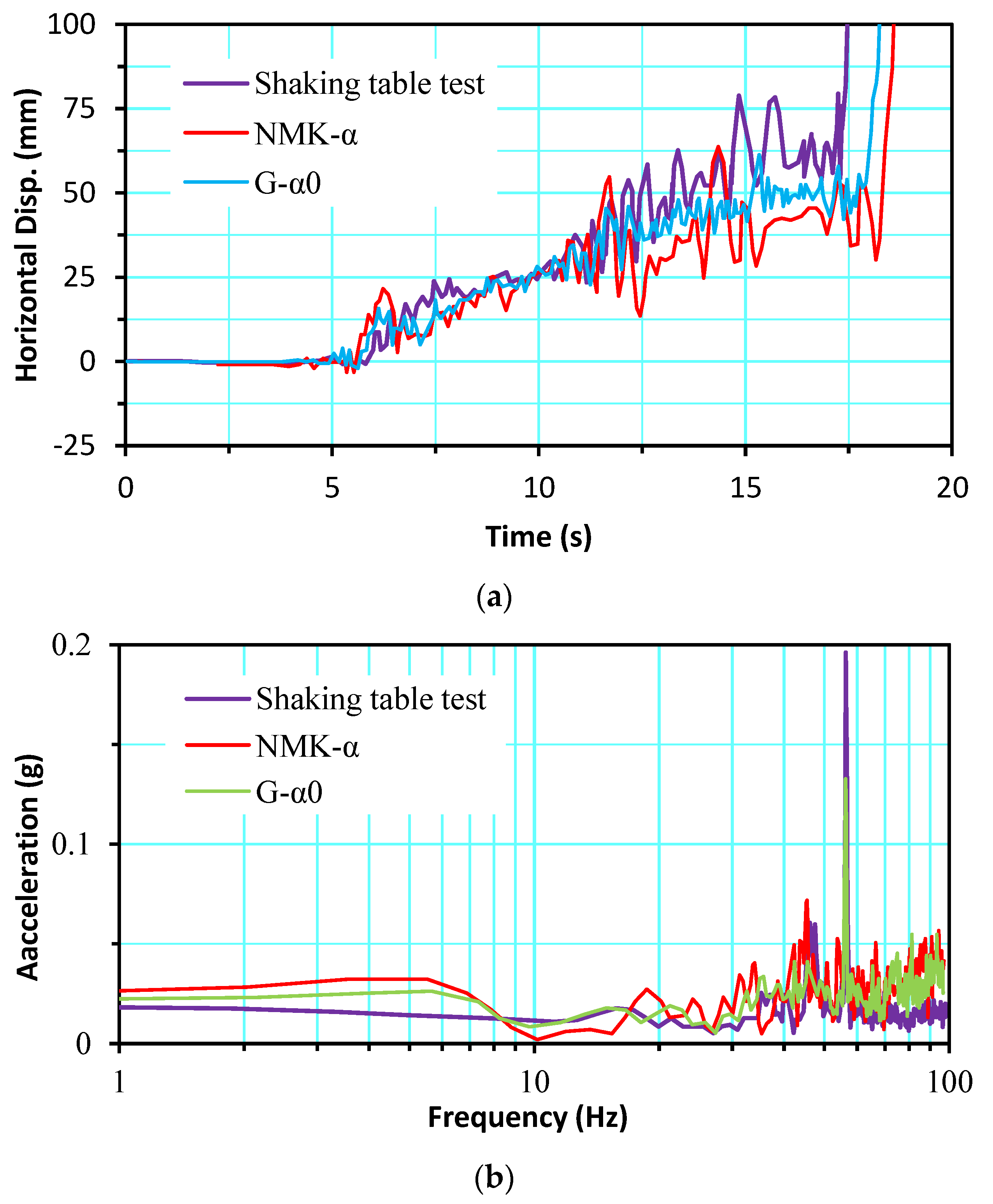
Compared with the experimental test results [38] (i.e., Figure 18) and the proposed G-α method using the NMM (i.e., Figure 19), it was found that the G-α₀ method could be used to simulate sliding and rotation (locking) of the block seen in the test well. Figure 20 shows the results of horizontal displacement and acceleration spectrum of the top block of the numerical methods and experiments. From these data, horizontal displacement and acceleration spectrum can be well expressed by the G-α₀ method. Thus, it was proven that the proposed G-α₀ method could well simulate the vibration response of assembled blocks. On the other hand, it was also proven that the G-α₀ method could be used to simulate the vibration response of the assembled blocks accurately.

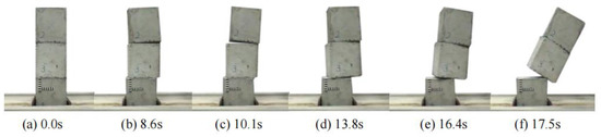
Figure 18. Behavior of the blocks under the shaking table test.

Figure 19. Simulated results of the model using the G-α₀ method. (a) 4.35 s; (b) 6.44 s; (c) 7.32 s; (d) 10.74 s; (e) 17.68 s; (f) 18.65 s.

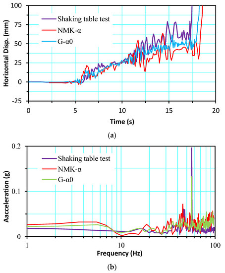
Figure 20. Comparisons of the results between the numerical and the shaking table test. (a) Horizontal displacement of the top block. (b) Horizontal acceleration spectrum of the top block.

4.4. Simulation of the Mechanical Behavior of Dynamical Tunneling

In this simulation, the mechanical behavior of inclined rock mass during dynamic tunnel construction was studied. Rock fractures are composed of many discontinuous, discrete blocks. The effect of the stress arch on the stress distribution and surface subsidence during dynamic tunneling was studied, and the calculation results compared with previous experiments [39].

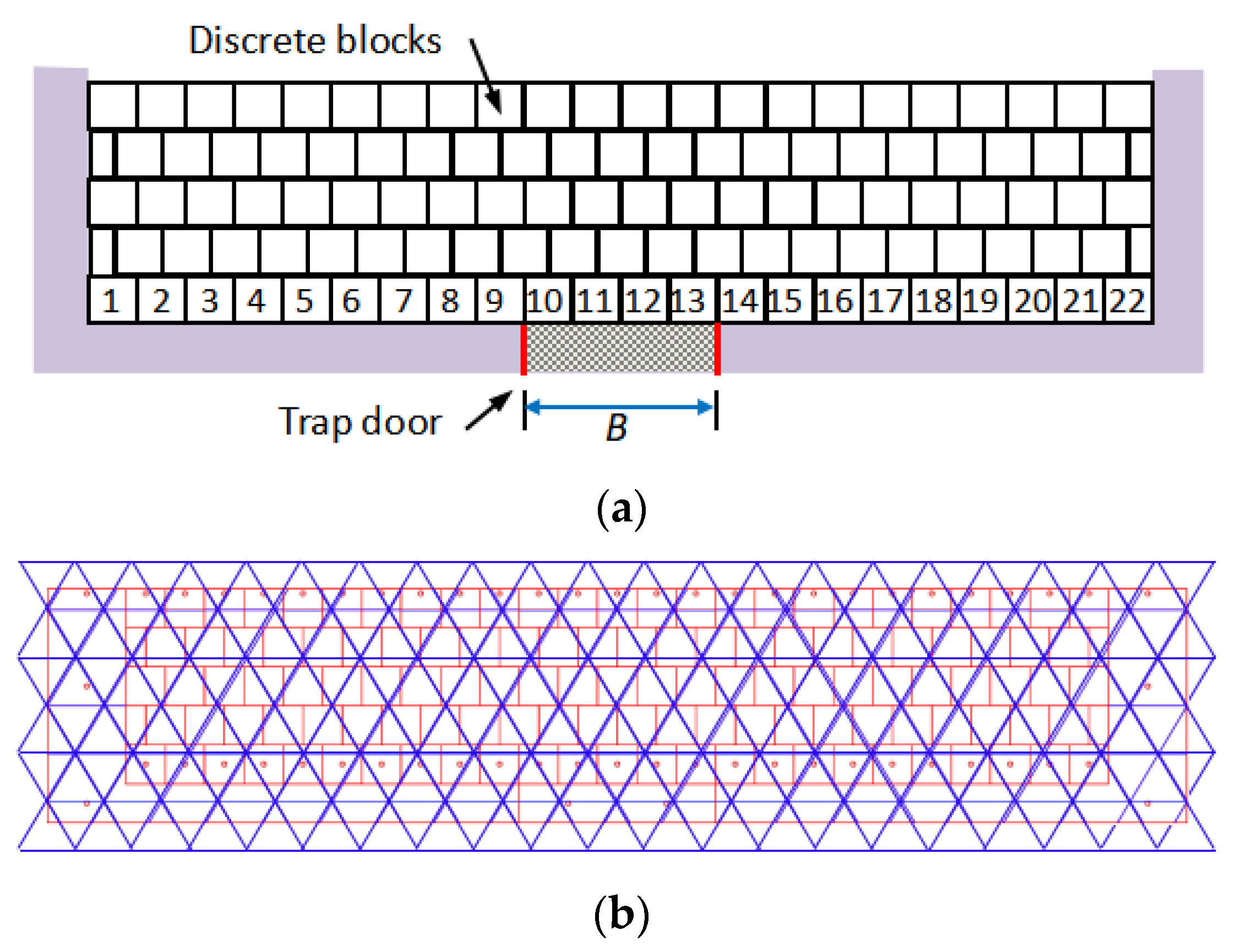
Figure 21 presents a simplified model of jointed rock masses with a dip angle of 0°. Both the depth of the discontinuous blocks and the width of trap door B were assumed to 200 mm. The input parameters of the modeling were: the Young’s modulus of 62 MPa, Poisson’s ratio of 0.15, unit density of 26.4 kN/m³, and the internal frictional angle of 20°. In the simulations, the effect of the deposit blocks is denoted by 10, 11, 12, and 13 on the vertical stress around the area of rock masses bottom was studied using the G-α and the three other methods, respectively. As presented in Figure 21b, 705 NMM elements and 130 blocks were divided using the FEM meshing technique, where a 2 mm gap was prescribed between the bottom of the blocks and trap door. Furthermore, in order to achieve numerical stability and save computational time, the kinetic damping of ${\theta }_{crit-1}=0.8033$ was used in the G-α₀, G-α₁, and G-α₂ methods, and ${\theta }_{crit-2}=0.8080$ was applied in the NMK-α method, respectively.

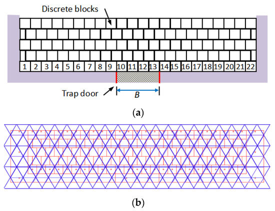
Figure 21. Block model for the simulations: (a) geometry of the model; (b) NMM mesh.

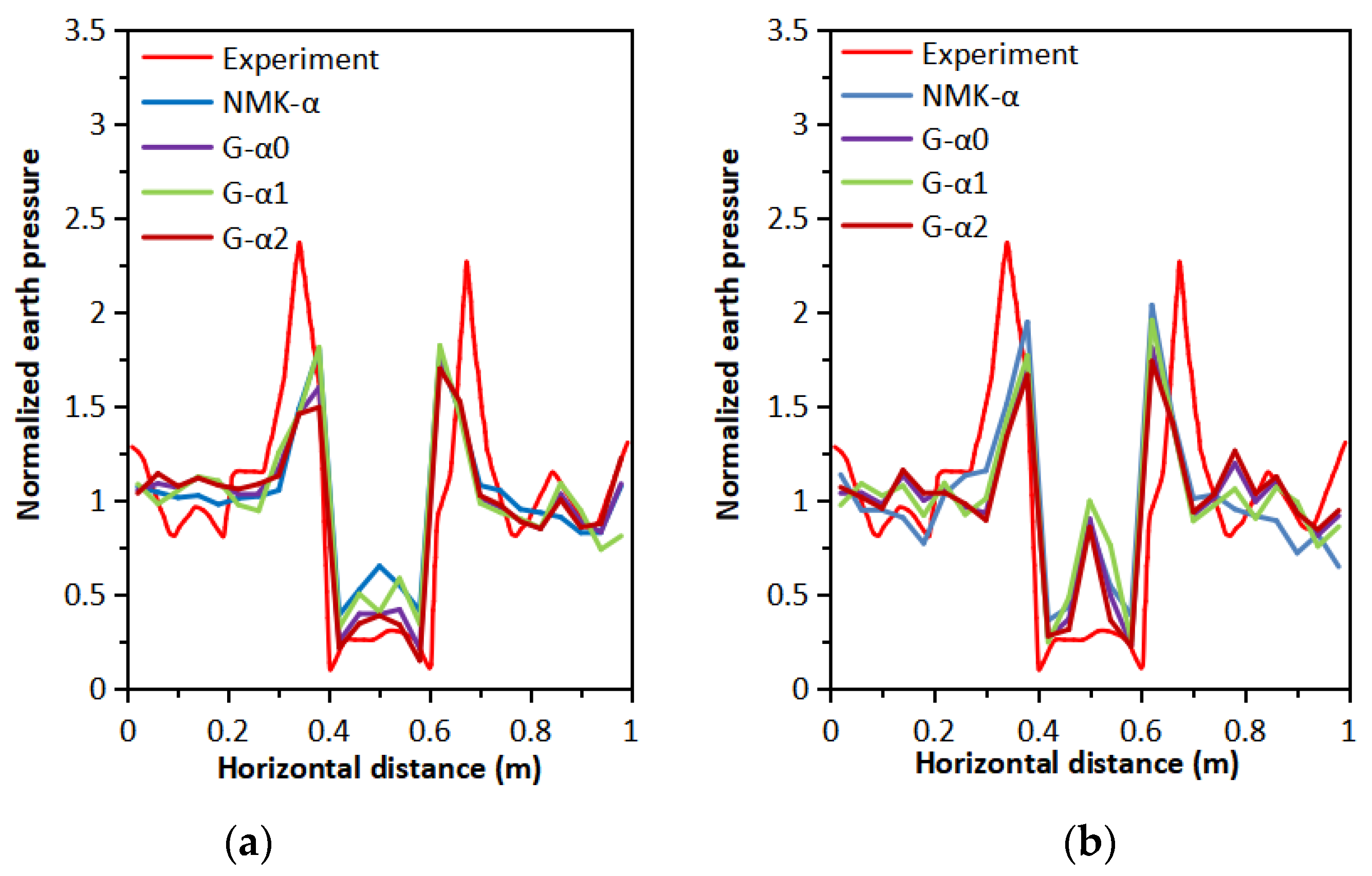
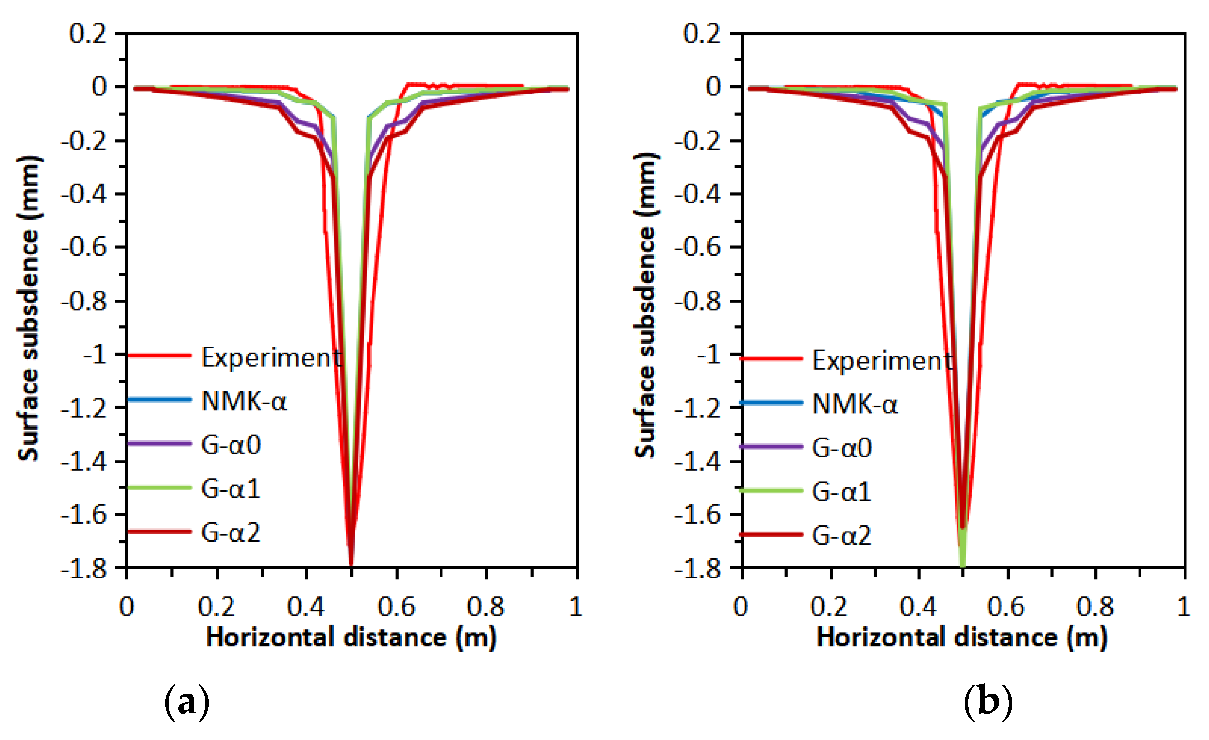
Figure 16 presents the normal stress distribution simulated by the referred methods using $\Delta t$ = 0.1 and $\Delta t$ = 0.01 ms, respectively. It was found that the normal stress distributions were symmetrical, and the simulated results were in agreement with the experiments. When $\Delta t$ = 0.01 ms was used in the computations, the local yield section [40] was found by the three referred algorithms. On the other hand, when a larger time step $\Delta t$ = 0.1 ms was applied to the modeling, the spurious oscillation became weaker and the simulated results were more accurate with the G-α method than that of the NMK-α method. When a smaller step time (i.e., $\Delta t$ = 0.01 ms) was employed, as shown in Figure 22b, the simulated results of the G-α₀, G-α₁, and G-α₂ methods were more stable than that of the NMK-α method. Figure 23 shows the simulated results of the surface subsidence by the above referred algorithms using the different time steps (i.e., $\Delta t$ = 0.1 ms and $\Delta t$ = 0.01 ms). Due to the numerical stability properties of the algorithms, the simulated results of the G-α algorithm still oscillated, but approached the experiments more than that of the NMK-α method.

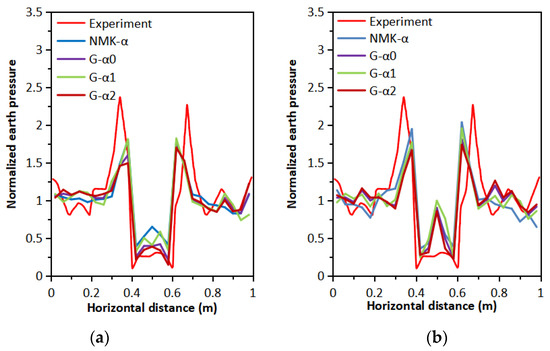
Figure 22. Normal stress distribution simulated by the referred methods: (a) $\Delta t$ = 0.1 ms; (b) $\Delta t$ = 0.01 ms.

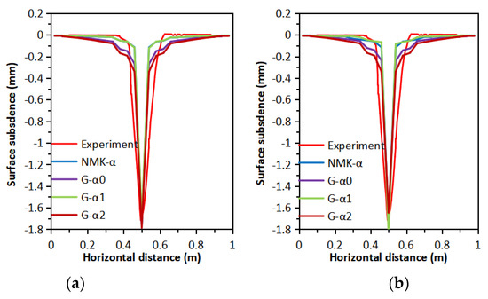
Figure 23. Surface subsidence simulated by the referred schemes: (a) $\Delta t$ = 0.1 ms; (b) $\Delta t$ = 0.01 ms.

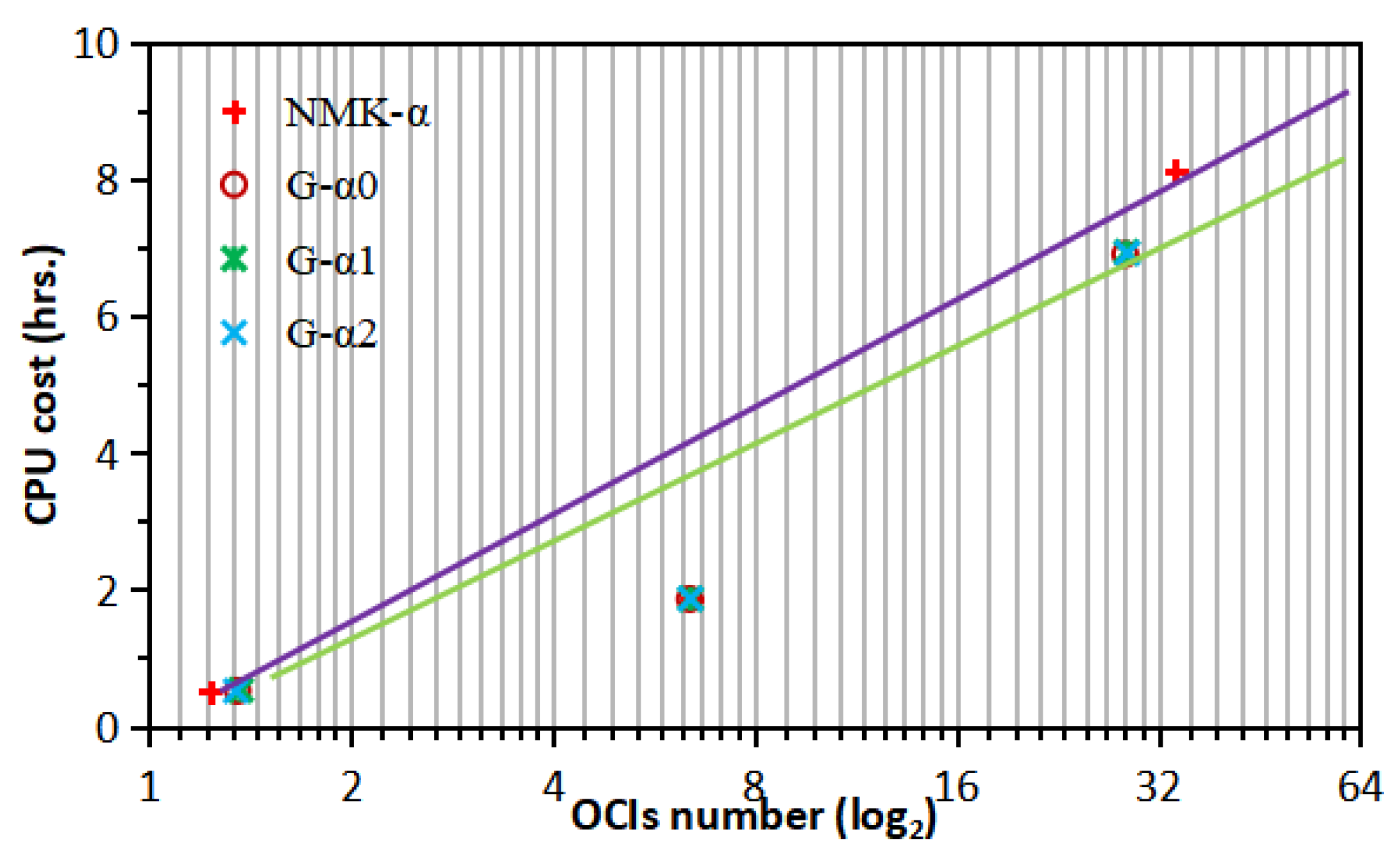
The computational cost of the OCIs using the referred time integration schemes was further calculated in the present study. As listed in Table 4, the CPU cost by the G-α algorithm significantly increased from 0.51839 to 6.90864 h while the number of OCIs from 13,537 to 285,273 with the time step $\Delta t$ = 1.0 ms to $\Delta t$ = 0.01 ms. Accordingly, the NMK-α algorithm had the same increase in terms of the CPU cost and the OCIs. As can be seen in Figure 24, the G-α schemes were more efficient than that of the traditional NMK-α method used in the NMM, not only in terms of the CPU time, but also the OCIs when the smaller time step (i.e., $\Delta t$ = 0.01 ms) was used. The G-α₀ method took a minimum of 6.90864 h compared with 8.13725 h (i.e., the maximum relative error was 15.10%) by the NMK-α method when the time step $\Delta t$ = 0.01 ms was used. The G-α scheme was more efficient with the increase in the OCIs caused by more discrete block contacts. These results suggest that except for the original NMK-α method used in the NMM, the G-algorithm can be effectively applied to models of tunnel behavior involving more complex discontinuous rock bodies.

Table 4. Comparisons of CPU cost and OCIs between the referred schemes.

Time Integration		$\Delta \mathit{t} = 1.0 \mathbf{ms}$		$\Delta \mathit{t} = 0.1 \mathbf{ms}$		$\Delta \mathit{t} = 0.01 \mathbf{ms}$
		OCIs	CPU Cost	OCIs	CPU Cost	OCIs	CPU Cost
NMK-α		12,336	0.50785	64,413	1.87334	339,547	8.13725
G-α	G-α1	13,682	0.52638	64,157	1.86636	286,845	6.93761
	G-α2	13,462	0.51523	64,088	1.86391	286,184	6.92388
	G-α0	13,537	0.51839	63,953	1.86116	285,273	6.90864

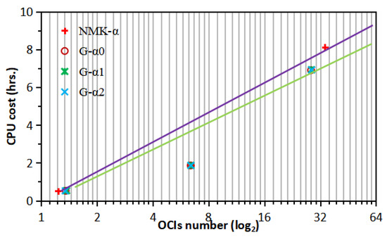
Figure 24. CPU cost versus OCIs by the referred algorithms.

5. Conclusions

In this paper, the generalized-α (G-α) time integration scheme was studied within the NMM frame, in which a thorough investigation was carried out to reveal the effects of the G-α₀, G-α₁, and G-α₂ methods and the Newmark method (i.e., NMK-α method) on the numerical stability and accuracy for dynamic simulations. For the first elastodynamic problem, the simulated results by the G-α scheme was in good agreement with the analytical solution. It was also found that the advantages of the G-α algorithm were apparent when the open–close iterations (OCIs) were applied for accurate contact analysis of the layered rock deflection. Comparing the simulated results of the behaviors of an assembled block system under seismic effect with the experiments, it was also clear that the G-α method could be applied to model the complicated discontinuous structural dynamic problems. Comparing the simulation results of the dynamical tunneling mechanical behavior with the experimental results, we also found that the G-α method can be used to simulate complex discontinuous structure dynamic problems. Furthermore, the convergence efficiency of the OCIs of the NMM at different time steps was investigated, with a significant decrease in the CPU time and OCIs of the NMK-α algorithm. The efficiency of the G-α algorithm implemented in the NMM code was proven, and it can be predicted that the G-α algorithm can simulate large scale discontinuous dynamic problems involving more nonlinear contacts.

References

- Hughes, T.J.R.; Hilber, H.M. Collocation, dissipation and [overshoot] for time integration schemes in structural dynamics. Earthq. Eng. Struct. Dyn. 1978, 6, 99–117. [Google Scholar] [CrossRef] [Green Version]
- Newmark, N.M. A Method of Computation for Structural Dynamics. J. Eng. Mech. Div. 1959, 85, 67–94. [Google Scholar] [CrossRef]
- Wilson, E.L.; Farhoomand, I.; Bathe, K.J. Non-linear dynamic analysis of complex structures. Earthq. Eng. Struct. Dyn. 1973, 1, 241–252. [Google Scholar] [CrossRef]
- Hilber, H.M.; Hughes, T.J.R.; Taylor, R.L. Improved numerical dissipation for time integration algorithms in structural dynamics. Earthq. Eng. Struct. Dyn. 1977, 5, 283–292. [Google Scholar] [CrossRef] [Green Version]
- Wood, W.L.; Bossak, M.; Zienkiewicz, O.C. An alpha modification of Newmark’s method. Int. J. Numer. Methods Eng. 1980, 15, 1562–1566. [Google Scholar] [CrossRef]
- Houbolt, J.C. A Recurrence Matrix Solution for the Dynamic Response of Elastic Aircraft. J. Aeronaut. Sci. 1950, 17, 540–550. [Google Scholar] [CrossRef]
- Bazzi, G.; Anderheggen, E. The ρ-family of algorithms for time-step integration with improved numerical dissipation. Earthq. Eng. Struct. Dyn. 1982, 10, 537–550. [Google Scholar] [CrossRef]
- Hoff, C.; Pahl, P. Development of an implicit method with numerical dissipation from a generalized single-step algorithm for structural dynamics. Comput. Methods Appl. Mech. Eng. 1988, 67, 367–385. [Google Scholar] [CrossRef]
- Chung, J.; Hulbert, G.M. A Time Integration Algorithm for Structural Dynamics with Improved Numerical Dissipation: The Generalized-α Method. J. Appl. Mech. 1993, 60, 371–375. [Google Scholar] [CrossRef]
- Shi, G.H. Discontinuous Deformation Analysis—A New Numerical Model for the Statics and Dynamics of Deformable Block Structures. Ph.D. Thesis, University of California, Berkeley, CA, USA, 1988. [Google Scholar]
- Jing, L. Formulation of discontinuous deformation analysis (DDA)—An implicit discrete element model for block systems. Eng. Geol. 1998, 49, 371–381. [Google Scholar] [CrossRef]
- Dahlquist, G.G. A special stability problem for linear multistep methods. BIT Numer. Math. 1963, 3, 27–43. [Google Scholar] [CrossRef]
- Bathe, K.-J.; Noh, G. Insight into an implicit time integration scheme for structural dynamics. Comput. Struct. 2012, 98–99, 1–6. [Google Scholar] [CrossRef]
- Bathe, K.-J. Conserving energy and momentum in nonlinear dynamics: A simple implicit time integration scheme. Comput. Struct. 2007, 85, 437–445. [Google Scholar] [CrossRef]
- Hulbert, G.M.; Jang, I. Automatic time step control algorithms for structural dynamics. Comput. Methods Appl. Mech. Eng. 1995, 126, 155–178. [Google Scholar] [CrossRef]
- Gobat, J.; Grosenbaugh, M. Application of the generalized-α method to the time integration of the cable dynamics equations. Comput. Methods Appl. Mech. Eng. 2001, 190, 4817–4829. [Google Scholar] [CrossRef]
- Yu, K.P. A new family of generalized-α time integration algorithms without overshoot for structural dynamics. Earthq. Eng. Struct. Dyn. 2008, 37, 1389–1409. [Google Scholar]
- Han, B.; Zdravkovic, L.; Kontoe, S. Stability investigation of the Generalised-α time integration method for dynamic coupled consolidation analysis. Comput. Geotech. 2015, 64, 83–95. [Google Scholar] [CrossRef] [Green Version]
- Tamma, K.K.; Zhou, X.; Sha, D. A theory of development and design of generalized integration operators for computational structural dynamics. Int. J. Numer. Methods Eng. 2001, 50, 1619–1664. [Google Scholar] [CrossRef]
- Shi, G.H. Manifold Method of Material Analysis; DTIC Document; Army Research Office Research Triangle Park NC: Durham, NC, USA, 1992. [Google Scholar]
- Shi, G.H. Modeling rock joints and blocks by manifold method. In Proceedings of the 33rd US Symposium on Rock Mechanics, Santa Fe, NM, USA, 3 June 1992. [Google Scholar]
- Chen, G.; Ohnishi, Y.; Ito, T. Development of high-order manifold method. Int. J. Numer. Methods Eng. 1998, 43, 685–712. [Google Scholar] [CrossRef]
- Zhang, H.; Li, L.; An, X.; Ma, G. Numerical analysis of 2-D crack propagation problems using the numerical manifold method. Eng. Anal. Bound. Elements 2010, 34, 41–50. [Google Scholar] [CrossRef]
- Ning, Y.; An, X.; Ma, G. Footwall slope stability analysis with the numerical manifold method. Int. J. Rock Mech. Min. Sci. 2011, 48, 964–975. [Google Scholar] [CrossRef]
- Wu, Z.; Wong, L.N.Y. Frictional crack initiation and propagation analysis using the numerical manifold method. Comput. Geotech. 2012, 39, 38–53. [Google Scholar] [CrossRef]
- Zheng, H.; Liu, Z.; Ge, X. Numerical manifold space of Hermitian form and application to Kirchhoff’s thin plate problems. Int. J. Numer. Methods Eng. 2013, 95, 721–739. [Google Scholar] [CrossRef]
- Qu, X.; Fu, G.; Ma, G. An explicit time integration scheme of numerical manifold method. Eng. Anal. Bound. Elements 2014, 48, 53–62. [Google Scholar] [CrossRef]
- Hu, M.; Rutqvist, J.; Wang, Y. A practical model for fluid flow in discrete-fracture porous media by using the numerical manifold method. Adv. Water Resour. 2016, 97, 38–51. [Google Scholar] [CrossRef] [Green Version]
- Li, X.; Zhang, Q.; Li, J.; Zhao, J. A numerical study of rock scratch tests using the particle-based numerical manifold method. Tunn. Undergr. Space Technol. 2018, 78, 106–114. [Google Scholar] [CrossRef]
- Ma, G.; Wang, H.; Fan, L.; Chen, Y. A unified pipe-network-based numerical manifold method for simulating immiscible two-phase flow in geological media. J. Hydrol. 2019, 568, 119–134. [Google Scholar] [CrossRef]
- Melenk, J.; Babuška, I. The partition of unity finite element method: Basic theory and applications. Comput. Methods Appl. Mech. Eng. 1996, 139, 289–314. [Google Scholar] [CrossRef] [Green Version]
- Zheng, H.; Liu, F.; Du, X. Complementarity problem arising from static growth of multiple cracks and MLS-based numerical manifold method. Comput. Methods Appl. Mech. Eng. 2015, 295, 150–171. [Google Scholar] [CrossRef]
- He, L.; An, X.; Liu, X.; Zhao, Z.; Yang, S. Augmented Numerical Manifold Method with implementation of flat-top partition of unity. Eng. Anal. Bound. Elements 2015, 61, 153–171. [Google Scholar] [CrossRef]
- An, X.; Li, L.; Ma, G.; Zhang, H. Prediction of rank deficiency in partition of unity-based methods with plane triangular or quadrilateral meshes. Comput. Methods Appl. Mech. Eng. 2011, 200, 665–674. [Google Scholar] [CrossRef]
- Doolin, D.M.; Sitar, N. Time Integration in Discontinuous Deformation Analysis. J. Eng. Mech. 2004, 130, 249–258. [Google Scholar] [CrossRef]
- Clough, R.W.; Penzien, J. Dynamics of Structures, 2nd ed.; McGraw-Hill: New York, NY, USA, 1993. [Google Scholar]
- Goodman, R.E. Introduction to Rock Mechanics, 2nd ed.; John Wiley & Sons: New York, NY, USA, 1989. [Google Scholar]
- Akao, S.; Ohnishi, Y.; Nishiyama, S.; Nishimura, T. Comprehending DDA for a block behavior under dynamic condition. In Proceedings of the 8th International Conference on Analysis of Discontinuous Deformation, Beijing, China, 17–19 August 2007. [Google Scholar]
- Murayama, S. Earth Pressure on Vertically Yielding Section in Sand Layer; Kyoto University: Kyoto, Japan, 1968. [Google Scholar]
- He, L.; Zhang, Q. Numerical investigation of arching mechanism to underground excavation in jointed rock mass. Tunn. Undergr. Space Technol. 2015, 50, 54–67. [Google Scholar] [CrossRef]
Publisher’s Note: MDPI stays neutral with regard to jurisdictional claims in published maps and institutional affiliations. |
© 2022 by the authors. Licensee MDPI, Basel, Switzerland. This article is an open access article distributed under the terms and conditions of the Creative Commons Attribution (CC BY) license (https://creativecommons.org/licenses/by/4.0/).