Prediction of Friction Degradation in Highways with Linear Mixed Models

Abstract

The development of a linear mixed model to describe the degradation of friction on flexible road pavements to be included in pavement management systems is the aim of this study. It also aims at showing that, at the network level, factors such as temperature, rainfall, hypsometry, type of layer, and geometric alignment features may influence the degradation of friction throughout time. A dataset from six districts of Portugal with 7204 sections was made available by the Ascendi Concession highway network. Linear mixed models with random effects in the intercept were developed for the two-level and three-level datasets involving time, section and district. While the three-level models are region-specific, the two-level models offer the possibility to be adopted to other areas. For both levels, two approaches were made: One integrating into the model only the variables inherent to traffic and climate conditions and the other including also the factors intrinsic to the highway characteristics. The prediction accuracy of the model was improved when the variables hypsometry, geometrical features, and type of layer were considered. Therefore, accurate predictions for friction evolution throughout time are available to assist the network manager to optimize the overall level of road safety.

1. Introduction

Road pavements are usually designed for a life cycle of 10 to 20 years. In this period, road agencies or transport departments are responsible for guaranteeing acceptable pavement quality standards. Among the most relevant parameters to assure road safety adopted by many of those departments are rutting [1], usually associated with structural performance, and friction or skid resistance [2], associated with functional performance. Many EU countries have developed national policies to control skid resistance in their networks. Some rely on skid resistance coefficient measurements, and others on correlations between road surface macrotexture depth and the skid resistance coefficient [3].

Besides that, many transport departments, road agencies, and researchers have dedicated their efforts to the development of friction degradation models. Currently, these models consider as predominant factors the texture, the average annual or cumulative daily traffic, the age of the surface course, and the polishing coefficient of the aggregates of the surface during a certain period [4,5,6,7].

Recently, the need for experimentally validated skid resistance prediction models accounting for tire and pavement surface texture characteristics and environmental factors was identified [8]. In this sense, more models were developed for several pavement treatments at various climate, traffic, and pavement conditions [6]. They were in accordance with previous studies based on long-term monitoring of friction, which mentioned that age of surface course, traffic volume, and climate of a section were directly related to friction, and other factors such as speed, temperature, tyre type and state (size, tread profile, tyre pressure rating), and type of road surface could affect pavement friction [6,9]. In asphalt mixtures, the binder also affects friction, but it has been considered in an early stage of pavement life [10], which justifies neglecting it in the friction prediction models. However, an asphalt mixture is a coated system with a nonlinear visco-elastoplastic response [11]. Researchers started only recently to look at it as so [12], seeking to improve friction modelling.

Further factors can influence the performance of friction over time, such as the type of layer [6,8], the road alignment, and profile characteristics whose relationship has not yet been adequately demonstrated [13], particularly in long-term studies (LTPP). Moreover, it was acknowledged that the level of skid resistance required for roads in operation should vary throughout the road depending on its geometry and other factors [14].

The methods used to model pavement degradation/performance indicators are many. They include stochastic methods such as the Markov chain and Bayesian methodology, linear or nonlinear regression and panel data/longitudinal models, or so-called mixed-effects models [15], and artificial intelligence modelling techniques.

The advantages of the mixed-effects models are several, namely greater flexibility, identification of temporal patterns of databases, the possibility of including predictors of temporal variation and iterations of variations of these predictors with time, and the possibility of testing the significance of the error [16,17,18].

Despite the advantages they present, these models have few applications to either model global or individual performance indicators. For example, Yu et al. [19] used linear mixed-effects models to predict future conditions of a specific pavement section, and Khraibani et al. [20] and Lorino et al. [17] developed nonlinear mixed-effects models to identify and quantify the impact of structural and climatic factors on cracking evolution. Regarding pavement skid resistance performance, from LTPP testing sections, Li et al. [6] developed both fixed- and random-effects models to evaluate and identify the most influential factors.

On the contrary, Markov chains are widely used as a probabilistic model to predict pavement performance [21,22,23], but they are not suitable for investigating the factors affecting the deterioration process. Artificial Intelligence (AI) techniques are also used to model pavement degradation [24,25,26] and friction precisely [27]. Due to the non-formulated nature of these techniques, the analysis of the factors is more complex and, therefore, less attractive for such a purpose.

Based on the literature review, the need to develop comprehensive and validated models adapted to local conditions to predict asphalt pavement friction is clear. This is due to the variety of local conditions and possibly the difficulty of accessing reliable databases with enough information along time. Moreover, enhanced regression modelling techniques offer the possibility of investigating the model’s significant factors in depth.

2. Study Methodology

The literature review showed the relevance of developing friction models that incorporate local condition variables and the advantages of using regression modelling approaches. Therefore, this study aimed to describe the friction degradation of flexible pavements and identify whether the traffic, climate conditions, pavement structure, geometric characteristics, and location influence behavior.

The study methodology consisted of two main phases: Introduction of study area and data to be modeled, and modelling approach to achieve the main objectives.

In the first phase, provided by a Portuguese motorway concessionary, a raw database was worked out and completed with climate data. A wide set of descriptive variables was defined, taking into account the literature review remarks and also the variables included in the friction models available. Therefore, five explanatory variable groups constitute the database: Traffic, climate conditions, pavement structure, geometric characteristics, and location. Descriptive statistics were carried out, and a correlation analysis was performed to identify the explanatory variables to be included in the model.

In the second phase, linear-mixed models with random effects in the intercept were described and fitted for the two- and three-level datasets. Level 3 introduces regional effects, level 2 distinguishes road sections, and level 1 represents the friction repeated measures made over time. Furthermore, for each level dataset, two approaches were made:

• the model considers only the variables inherent to traffic and climate conditions;
• the model, in addition to the previous variables, includes factors intrinsic to highway characteristics.

Thus, in total, four Linear Mixed Models (LMMs) were developed and compared to find the model that provides a better fit to the data.

Finally, the cross-validation technique was used to evaluate the predictive performance of all models.

In the next sections, these two main study phases are described in detail, and the results are examined.

3. Materials and Methods

3.1. Friction Measurement

In this study, the wet skid resistance was measured with a Grip Tester, according to the technical standard CEN/TS 15901-7:2009 [2]. The device is a trailer with two drive wheels and a single small test wheel that was towed behind a vehicle (Figure 1). The test wheel is mounted on a stub axle and is mechanically braked by a fixed gear and chain system with a ratio of 27:32 in relation to the drive wheels so that there is a slip ratio of just over 15%. The static load on the test wheel is (50 ± 30) N. The test wheel tyre has a smooth tread. The two drive wheels are mounted on the main axle, which also carries a toothed wheel. Water is deposited in front of the test tyre from a water tank fitted with a control valve. To the trailer are coupled systems to continuously measure and store the distance and horizontal drag and vertical load forces. The friction coefficient, known as the Grip Number (GN), is calculated as the rate vertical/drag load forces. The test was carried out in wet conditions with the vehicle operating at 50 km/h.

3.2. Data Collection

The data was collected in the highway network of the Portuguese concessionaire Ascendi on different roads with at least two traffic lanes in each direction, which are located in six districts: Aveiro, Braga, Guarda, Porto, Vila Real, and Viseu, as shown in Figure 2. Thus, they are inserted in different climate environments and topographic conditions, but they were constructed mostly with granite aggregates, as they are abundant in those regions.

As the quality control plan for this concessionary establishes that friction monitoring campaigns have to be carried out at 100 m sections every four years, sections with 100 m length were adopted. A sample with a total of 7204 pavement sections, each one identified by the corresponding kilometric point (PK), was made available for this study. Three monitoring campaigns were included in the study, times 0, 1, and 2. According to the operation and maintenance contract, friction measurements are carried out in each section approximately in the same period. The first measurements (time 0) were carried out 6 to 8 months after the road opened to traffic and after that, every four years. Therefore, with the first measurements, it is expected to capture the maximum friction, with the second (time 1) the equilibrium phase, and with the third (time 2), it is expected to capture friction changes.

In this period, in all sections, there were no maintenance operations on the pavement. After that time (eight years), it is common practice to carry out maintenance operations on highways that alter the pavement surface characteristics.

3.3. Description of the Database

The variables characterizing each 100 m section were grouped in a database as follows: Pavement structure (type of surface course); traffic (accumulated or annual average daily, light and heavy vehicles, and day or night); climate conditions (temperature, precipitation, and relative humidity of the air); geometric characteristics of the vertical and horizontal alignments (plan, profile), and the lane and hypsometry. Some of these variables were identified in the state-of-the-art review; others were defined according to the objectives of the work.

3.3.1. Type of Surface Course

The structure of the pavement is crucial information to the analysis of its performance. However, as this study intends to develop prediction models for the degradation of friction in road pavements, only the type of surface course is described in

Table 1. Categories of the explanatory variable type of surface course.

Categories	Description
PA	Porous asphalt (PA 12.5).
GGA.BMR	Gap-graded asphalt concrete (GGA) with bitumen modified with a high percentage of Rubber Modified Binder (BMR).
GGAC	Gap gradded asphalt concrete surface course (AC10surf) and (AC14surf).

.

3.3.2. Traffic

Since any road pavement is designed to support a determined traffic volume, on the most requested lane, obtained from a traffic study, therefore adding uncertainty to the data, in this study, real data concerning the traffic circulating on the highway were used. Actual traffic data were collected using automatic vehicle counter systems that are installed on highways and toll plazas. The selected traffic variables are described in

Table 2. Traffic explanatory variables.

Variable	Description
AADT	Annual average daily traffic (vehic./day × 106) in the year of the observation (t = 0, t = 1, t = 2). Calculated as the average 24-h traffic volume at a given location over a full 365-day year.
Ac.ADT	Accumulated annual daily traffic (vehic. × 106), until the time of the observation (t = 0, t = 1, t = 2). Represents the total number of vehicles that cross a section up to a given moment.
Ac.ADT/direction	Accumulated annual daily traffic per direction of circulation (vehic./direction × 106), until the time of the observation (t = 0, t = 1, t = 2). This is the Ac.ADT divided by 2.
Ac.ADT/direction/lane	Accumulated annual daily traffic per direction and per lane (vehic./direction/lane × 106), until the time of the observation (t = 0, t = 1, t = 2). For sections with two lanes: RL = 95% and LL = 5%, and three lanes: SL = 80%, RL = 15% and LL = 5%.
Ac.ADT heavy	Accumulated annual daily heavy traffic (heavy vehic. × 106), until the time of the observation (t = 0, t = 1, t = 2). Heavy vehicles are those with more than two axles and with a height greater than or equal to 1.10 m. Represents the total number of heavy vehicles that cross a section up to a given moment.
Ac.ADT heavy/lane	Accumulated annual daily heavy traffic per lane (heavy vehic./lane × 106), until the time of the observation (t = 0, t = 1, t = 2). Represents the total number of heavy vehicles that cross a section up to a given moment in a given lane as a percentage of the total heavy vehicles circulating in each direction. For sections with two lanes: RL = 95% and LL = 5%, and three lanes: SL = 80%, RL = 15% and LL = 5%.
Ac.ADT heavy_daytime	Accumulated annual daily heavy traffic that circulated in the daytime period in a given lane, between 07:00 and 19:00, (heavy vehic._daytime × 106), until the time of the observation (t = 0, t = 1, t = 2).
Ac.ADT heavy_nighttime	Accumulated annual daily heavy traffic, that circulated in the night period between 19:00 and 07:00 in a given lane, (heavy vehic._nighttime × 106), until the time of the observation (t = 0, t = 1, t = 2).

RL: right lane; LL: left lane; SL: slow lane; t: time.

.

3.3.3. Climate Conditions

Temperature, particularly its variation, influences the performance of bituminous mixes. Therefore, it was considered adequate to gather all the data available on the Portuguese Institute of the Sea and Atmosphere (IPMA) site to characterize it, as it covers a wide area and can be accessed by everybody. The record of climate normals (average values) concerning the 1971–2000 period [28] was used to set the temperature factors.

Precipitation was another climate factor that has been regarded. For that, the averages of the total quantity of precipitation (P) and the maximum daily quantity of precipitation (PM), which are available in the Climatological Atlas of the Iberian Peninsula or Iberian Climate Atlas (ACI) [28] were used. The variable relative humidity (RH), available in Portal do Clima [29], was also considered. Thus, the values considered for the climate variables correspond to the month in which friction was measured and to the zone or district where it is inserted.

Table 3. Explanatory variables concerning the climate conditions corresponding to the month in which friction was measured and the zone or district where it is inserted.

Variables	Description
Higher max temp	Higher value of the maximum temperature, in °C.
Average max temp	Average maximum temperature, in °C.
Average med temp	Average mean temperature, in °C.
Average min temp	Average minimum temperature, in °C.
Lower min temp	Lower value of the minimum temperature, in °C.
Average No. days temp max30	Average number of days with maximum temperature ≥30 °C.
Average No. days temp max25	Average number of days with maximum temperature ≥25 °C.
Average No. days temp min20	Average number of days with minimum temperature ≥20 °C.
Average No. days temp min0	Average number of days with minimum temperature ≤0 °C.
Ac. No. days temp max30	Accumulated number of days with maximum temperature ≥30 °C.
Ac. No. days temp max25	Accumulated number of days with maximum temperature ≥25 °C.
Ac. No. days temp min20	Accumulated number of days with maximum temperature ≥20 °C.
Ac. No. days temp min0	Accumulated number of days with minimum temperature ≤0 °C.
P	Average of the total quantity of precipitation (mm).
PM	Daily maximum quantity of precipitation (mm).
RH	Relative humidity of the air (%).

describes all the variables concerning climate conditions.

A note about climate change is justified at this point. According to the Portuguese Meteorological Institute, up to 2040, in the study region, the annual average temperature will increase 1 °C in comparison to the 1971–2000 period. As the measurements were done in the last decade, it is acceptable to say that changes are small and the data can be used for modelling purposes. Furthermore, according to Anupam et al. [30], rough surfaces are expected to compensate for the lower hysteretic friction that characterizes friction measurements at higher temperatures. Therefore, as the surface courses included in this study are rough, the effect of temperature in each section (not between sections inserted in distinct areas) is small. Measurements carried out on similar roads of the same regions showed that friction variation could be neglected in the short term, even though the main factors that affect it were introduced and exhaustively analysed in the modelling procedure, as the number of climate variables suggests. Moreover, the model formulation includes a random effect associated with each 100 m section to introduce an extra source of variability into the model.

3.3.4. Geometric Characteristics

When a road alignment (plan and profile) is designed, multiple relations between the alignment and the environment where it will be implanted should be considered to ensure aspects such as the inherent costs of construction and operation, the circulation speed, the safety, and the comfort of the users. Therefore, it becomes relevant to characterize the highway sections according to the geometrical features to establish the effect of those design decisions on friction.

Table 4. Explanatory variables of the characteristics of the highway.

Variables	Categories	Description
Lane	Longitudinal area of the lane devoted to the circulation of vehicles; this variable is characterized by:
	LL	Left lane located close to the highway axis.
	RL	Right lane in highways or highway sections with two traffic lanes in the same direction.
	SL	Slow lane in highways or highway sections with three or more traffic lanes, for the circulation of cargo heavy vehicles or sets of vehicles whose length exceeds 7 m.
Plan	Corresponds to the horizontal characteristics in the highway (plan view) and is characterized by:
	SA	Straight alignment; this is the straight line that defines the plant alignment (∞).
	C	Clothoid, is the transition curve and is an adimensional parameter.
	CC	Circular curve, is the curve alignment of constant radius (m).
Profile	Corresponds to the characteristics of the vertical alignment of the highway (profile view); this variable is characterized by:
	S	Slope, this is the tangent of the angle formed with the horizontal (%).
	Ccc	Concave concordance curve, is the minimum radius of the concave concordances (m).
	Ccv	Convex concordance curve, is the minimum radius of the convex concordances (m).
Hypsometry	Describes the distribution of elevation of land with respect to sea level within an area of interest; his variable is characterized by:
	Low Altitude	Area where a section belongs to whose hypsometric curves are inserted in the interval [0, 200 m].
	Medium Altitudes	Area where a section belongs to whose hypsometric curves are inserted in the interval [200, 2000 m].

presents the variables related to the characteristics of the highway and also hypsometry as it is related to the altitude of each section.

3.4. Data Analysis

3.4.1. Descriptive Data Analysis

In this subsection, the descriptive analysis of the variables is presented. Firstly, a box plot illustrating how the dependent variable (friction) changed in time is presented in Figure 3. As can be seen, there is an apparent decrease in the median of the friction with time. To confirm that, a Kruskall–Wallis test was conducted. The test results showed statistically significant differences in the median of friction among the three times (p-value < 0.001). Furthermore, the friction of period 2 is statistically lower than the friction of periods 0 and 1 (Turkey’s HSD test, p-value < 0.001). This demonstrates that the parameter friction has a typical performance regarding the asphalt pavements.

As an example, Figure 4 shows observed friction values versus time for some pavement sections. The measurements of the same section are connected with lines. For each section, a distinct linear decrease of friction with time is shown, and considerable variation exists among sections.

A statistical summary of the quantitative variables is provided in

Table 5. Statistical summary of the quantitative variables.

Variables	Minimum	Maximum	Mean	Median	Standard Deviation	Coefficient of Variation
Friction	0.2400	0.9600	0.60	0.5900	0.13	0.22
AADT	0.0016	0.3290	0.0546	0.0412	0.0574	1.0511
Ac.ADT	0.0722	120.0850	18.9549	15.0523	20.9676	1.1062
Ac.ADT/direction	0.0361	60.0425	9.4775	7.5262	10.4838	1.1062
Ac.ADT/direction/lane	0.0018	57.0404	5.0233	0.7034	8.2631	1.6449
Ac.ADT heavy	0.0036	6.0043	0.9477	0.7526	1.0484	1.1062
Ac.ADT heavy/lane	0.0002	0.3002	0.0474	0.0376	0.0524	1.1062
Ac.ADT heavy_daytime	0.0001	0.2101	0.0332	0.0263	0.0367	1.1062
Ac.ADT heavy_nighttime	0.0001	0.0901	0.0142	0.0113	0.0157	1.1062
Higher max temp	22.00	40.50	32.43	34.00	6.23	0.19
Average max temp	11.80	29.20	20.72	20.90	5.13	0.25
Average med temp	7.70	21.40	15.64	16.40	4.33	0.28
Average min temp	3.50	16.00	10.57	11.50	3.77	0.36
Lower min temp	−7.30	11.40	1.76	1.40	4.65	2.64
Average No. days temp max30	0.00	14.70	2.92	0.80	4.22	1.45
Average No. days temp max25	0.00	25.80	7.74	5.60	8.46	1.09
Average No. days temp min20	0.00	1.50	0.29	0.00	0.42	1.44
Average No. days temp min0	0.00	4.90	0.53	0.00	1.04	1.98
Ac. No. days temp max30	7.40	44.60	22.25	13.90	13.35	0.60
Ac. No. days temp max25	41.00	99.00	66.83	49.40	24.23	0.36
Ac. No. days temp min20	1.00	5.30	2.11	1.70	1.13	0.54
Ac. No. days temp min0	2.30	39.90	14.07	11.90	12.57	0.89
P	11.80	231.15	83.39	82.60	57.27	0.69
PM	38.00	103.16	64.24	66.00	15.89	0.25
RH	30.00	70.00	51.46	50.00	12.64	0.25

. As can be seen, the average of the friction is 0.6 GN and ranges from 0.24 GN to a maximum of 0.96 GN. Regarding the traffic variables, the difference between the highest and lowest value of the annual average daily traffic (AADT) up to the observation year is 0.3274 × 10⁶ vehicles, showing a large increase over time. Moreover, according to the Portuguese Road Pavement Design Manual [31], the minimum value for the accumulated annual average daily traffic of heavy vehicles (Ac.ADT heavy) fits within the traffic class T3 and T4 (300–800 heavy vehicles), therefore in an intermediate traffic level at the beginning of the life of the pavements.

In the case of temperature data, the higher value of the maximum temperature (higher max temp), the average maximum temperature (average max temp), and the lower value of the minimum temperature (lower min temp) are those that present the largest difference between the minimum and the maximum value. This situation also occurs for the accumulated number of days with a maximum temperature of 25 °C (Ac. No. days temp max25).

The difference between the highest and lowest value of the average of the total quantity of precipitation (P) is 219.4 mm, and the average of the relative humidity of the air (RH) is 51.5%. This shows that climate variables address a broad set of conditions that are representative of the Portuguese weather.

Regarding the qualitative variables, the absolute frequency (number of events) and relative frequency (absolute frequency normalized by the total number of events) are described in

Table 6. Frequencies of the qualitative variables.

Variable	Categories	Absolute Frequency	Relative Frequency
Lane	LL	3 367	46.7
	RL	3 326	46.2
	SL	511	7.1
Plan	SA	2 322	32.2
	C	2 209	30.7
	CC	2 673	37.1
Profile	S	4 131	57.3
	Ccc	1 379	23.5
	Ccv	1 694	19.1
Layer	GGAC	3 951	54.8
	PA	2 850	39.6
	GGA.BMR	403	5.6
Hypsometry	Low Altitude	2 411	33.5
	Medium Altitudes	4 793	66.5

.

Only 7.1% of the sections typify the additional heavy vehicles lane (SL). About 37% of the sections are in a circular curve (CC), and the number of sections in straight alignment (SA) or clothoid (C) is about 31%, whereas the profile is characterized by 57% of the sections in slope (S).

The number of sections with a gap-graded concrete surface course (GGAC) is much higher (54.8%) than the number of sections with a gap-graded asphalt concrete modified by a high percentage Rubber Modified Binder (GGA.BMR) (5.6%), and most of the sections, about 67%, are located at medium altitudes.

3.4.2. Correlation of the Variables

Given the relatively large number of explanatory variables, a correlation analysis was performed to identify which explanatory variables are highly correlated with the response variable (friction) to be included in the model. Correlations among variables were tested depending on the Pearson’s correlation coefficient, which measures the direction and strength of the linear relationship between two continuous numerical variables.

Table 7. Correlation between the dependent variable and some explanatory variables (coefficient of Pearson).

Explanatory Variables	Pearson Coefficient (rs)	Significance of the Correlation (Bilateral)
Ac.ADT	−0.645	<0.01
Higher max temp	0.222	<0.01
Average no. days temp max25	0.223	<0.01
P	−0.12	<0.01
RH	0.366	<0.01

presents the Pearson’s correlation coefficient (rs) of response variable and all explanatory variables highly correlated with the response variable. Therefore, these variables are selected as the explanatory variables in regression modelling and will be included in the mixed model as the fixed effect covariates.

The results analysis showed that the traffic variable with the highest linear relation with the response variable was Ac.ADT (with rs = −0.645, p-value < 0.01), and the variables related to climate conditions—the higher max temp (with rs = 0.222, p-value < 0.01); average No. days temp max25 (with rs = 0.223, p-value < 0.01); P (with rs = −0.12, p-value < 0.01) and RH (with rs = 0.366, p-value < 0.01)—are significantly correlated (p-value less than 0.05) with the dependent variable (friction).

For example, the mean profiles of friction values for all sections versus two of the explanatory variables are provided in Figure 5. These plots show that the mean friction decreases linearly with Accumulated Annual Daily Traffic (Ac.ADT) and increases linearly with average number of days with maximum temperature ≥25 °C (average No. days temp max25).

4. Modelling Approach

4.1. Model Formulation

Linear mixed-effects models (LMMs) are mixed-effects models in which both the fixed and the random effects occur linearly in the model function.

LMMs are particularly appropriate for the analysis of nested structured data, as in this study. Kilometric points (PK) are nested within districts, and repeated measures are collected on the same kilometric point over time.

These models extend linear models by incorporating random effects, which can be regarded as additional error terms, to explain the correlation between observations within the same group. In this study, dealing with a large number of kilometric points, some degree of unobserved heterogeneity is present. The unobserved heterogeneity among pavement sections was accounted for by using random intercept models.

The linear mixed-effects model expresses the i-th kilometric point as [29]:

$$Y_i=X_i\mathsf{\beta }+b_i+{\mathsf{\epsilon }}_i, i = 1,\dots , \mathrm{n}$$

(1)

where:

Y_i 

${\left(Y_{i1}\dots Y_{i{T}_i}\right)}^T$ represents a vector (of size T_i × 1) of responses (friction) for the i-th kilometric point;

X_i 

is the known fixed-effects covariates matrix (of size T_i × p);

β 

is a vector (of size p × 1) of unknown regression coefficients (or fixed-effects parameters);

b_i 

is a vector (of size q × 1) of random-effects associated with the i-th kilometric point;

ε_i 

represents an error vector (of size T_i × 1) of n residuals associated with an observed response for the i-th kilometric point.

Moreover:

b_i 

~Nq (0, D)

ε_i 

~N_Ti (0, R_i)

b_i e ε_i 

are independent for the same i-th kilometric point and of each other.

where D is the q × q covariance matrix for the random effects, and R_i is the T_i × T_i covariance matrix of the errors in kilometric point i.

In general terms, the maximum likelihood methods (Maximum Likelihood—ML; or Restricted Maximum Likelihood—REML) are used to obtain estimates of the parameters in LMMs. However, ML estimates of the covariance parameters are biased, whereas REML estimates are not. This aspect makes it impossible to compare mixed linear models with different fixed-effects structures based on the restricted maximum likelihood function [32].

Following the methodology described in Pinheiro and Bates [32], the significance of fixed effects’ terms in the model is assessed by conditional F-tests using a sequential sum of squares.

When two different models are nested (they differ only by adding more parameters to the fixed effects structure), a Likelihood Ratio Test (LRT) comparing the log-likelihood values between two models is used to test the superiority of different models. This test is only valid if the fixed effects on both models were estimated by the ML method [32].

Akaike’s Information Criterion [33] and Bayesian Information Criterion [34] are also used to compare several alternative models. These criteria are based on the maximum likelihood function, the number of parameters, and the number of observations, or equivalently, the sample size. The lowest value for both criteria indicates the best fit [16,32]. In this study, Akaike’s Information Criterion (AIC) and Bayesian Information Criterion (BIC) are used to choose the most appropriate structure for the covariance matrix of the errors (R_i), which describes the structure of the correlation among data points within kilometric points.

Cross-validation is a technique used to evaluate predictive models by partitioning the original sample into a training set to train the model, and a test set to evaluate it. The cross-validation methods for assessing model performance are the holdout method, the k-fold method, and the leave-one-out method. In k-fold cross-validation, the original sample is randomly partitioned into k equal sized subsamples. One sample is used to train the model, and the remaining ones are used to test it later to quantify the prediction error as the mean squared difference between the observed and the predicted outcome values. The k-fold method is considered one of the most robust methods for estimating model accuracy, as it evaluates the performance of the model in different subsets of training data [35]. Thus, it was adopted in this study.

The Root Mean Squared Error (RMSE), the Mean Absolute Error (MAE), and the Mean Bias Error (MBE) were used to assess models’ predictive performance. A smaller RMSE, MAE, or MBE value indicates a more accurate prediction.

All statistical analyses were performed using the R statistical software (version 3.5.0) [36] and the Statistical Package for the Social Sciences (version 24) [37].

4.2. Modelling Results

Using AIC and BIC, the independent structure was selected (this structure assumes no correlation between observations within kilometric points).

4.2.1. Linear Mixed Models for Two Levels of the Dataset (Models P)

First, the null model (no covariates) was fitted (Equation (2)).

$${\mathrm{Friction}}_{ti}={\mathsf{\beta }}_0+b_{0i}+{ \mathsf{\epsilon }}_{ti}$$

(2)

${\mathrm{Friction}}_{ti}$ is the dependent variable in time (t) in the kilometric point (i).

where $b_{0i} ~ N \left(0,{ \mathsf{\sigma }}_P^2\right) , {\mathsf{\epsilon }}_{ti}~ N \left(0,{ \mathsf{\sigma }}_{\mathsf{\epsilon }}^2\right)$, $i=1,\dots ,7204$ and $t=0, 1,2$.

This model is useful for deciding whether a random-effects model might be appropriate for the data.

Table 8. Results of the friction models P for the two-level Dataset.

Models P	Null Model P			Model P_I			Model P_II
Fixed-Effect Parameter	Estimate (β)	Standard Error	p-Value	Estimate (β)	Standard Error	p-Value	Estimate (β)	Standard Error	p-Value
Intercept	0.5960	0.0018	<0.0001	0.5068	0.0138	<0.0001	0.7800	0.0098	<0.0001
Time	–	–	–	−0.0625	0.0011	<0.0001	−0.0646	0.0011	<0.0001
Ac.ADT	–	–	–	−0.0012	0.0001	<0.0001	−0.0010	0.0000	<0.0001
Higher max temp	–	–	–	0.0039	0.0003	<0.0001	0.0039	0.0003	<0.0001
Average No. days temp max25	–	–	–	−0.0091	0.0002	<0.0001	−0.0095	0.0002	<0.0001
P	–	–	–	−0.0006	0.0000	<0.0001	−0.0007	0.0000	<0.0001
RH	–	–	–	0.0032	0.0002	<0.0001	–	–	–
Lane (ref: LL)	–	–	–	–	–	–	–	–	–
(Lane = RL)	–	–	–	–	–	–	−0.0394	0.0010	<0.0001
(Lane = SL)	–	–	–	–	–	–	−0.0250	0.0020	<0.0001
Plan (ref: SA)	–	–	–	–	–	–	–	–	–
(Plant = C)	–	–	–	–	–	–	−0.0040	0.0029	0.1619
(Plant = CC)	–	–	–	–	–	–	−0.0128	0.0027	<0.0001
Profile (ref: Ccc)	–	–	–	–	–	–	–	–	–
(Profile =Ccv)	–	–	–	–	–	–	0.0091	0.0035	0.0100
(Profile = S)	–	–	–	–	–	–	0.0024	0.0030	0.4380
Layer (ref: GGAC)	–	–	–	–	–	–	–	–	–
(Layer = PA)	–	–	–	–	–	–	−0.0787	0.0026	<0.0001
(Layer = GGA.RMB)	–	–	–	–	–	–	0.0086	0.0062	0.1625
Hypsometry (ref: Medium Altitudes)	–	–	–	–	–	–	–	–	–
(Hypsometry = Low Altitudes)	–	–	–	–	–	–	−0.1410	0.0029	<0.0001
Random Parameters	Estimate	IC 95%		Estimate	IC 95%		Estimate	IC 95%
${\mathsf{\sigma }}_P^2$	0.0049	(0.0045; 0.0053)		0.0063	(0.0059; 0.0068)		0.0019	(0.0017; 0.0020)
${\mathsf{\sigma }}_{\mathsf{\epsilon }}^2$	0.0119	(0.0117; 0.0121)		0.0051	(0.0050; 0.0052)		0.0047	(0.0046; 0.0048)

presents the parameter estimates, their corresponding standard error, and the p-value for this model.

Regarding the null model, the Portuguese National Road Administration has established a minimum friction standard value of 0.60 GN when t = 0. The intercept parameter estimates reflect it as it is close to this value.

Since ${\mathsf{\sigma }}_P^2=$0.0049 and ${\mathsf{\sigma }}_{\mathsf{\epsilon }}^2=0.119$, then 29.16% (0.0049/(0.0119 + 0.0049)) of the data variation is explained by allowing the intercept to vary across sections, indicating that unobserved heterogeneity among pavement sections is best captured by using a random-intercept model.

First, the Model P_I (using only the variables inherent to traffic and climate conditions) was fitted.

For Model P_I (Equation (3)), the statistically significant covariates were: Time, Ac.ADT, higher max temp, average no. days temp max25, P, and RH. This can be written as:

$$\begin{array}{ll}{\mathrm{Friction}}_{ti}={\mathsf{\beta }}_0& +{\mathsf{\beta }}_1{ \mathrm{Time}}_{ti} +{ \mathsf{\beta }}_2 \mathrm{Ac}.{\mathrm{ADT}}_{ti}+{ \mathsf{\beta }}_3 {\mathrm{Higher} \max \mathrm{temp}}_{ti}+{ \mathsf{\beta }}_4 \mathrm{Average} \mathrm{No}. \mathrm{days} \mathrm{temp} \max {25}_{ti}\\ & +{ \mathsf{\beta }}_5 P_{ti} +{ \mathsf{\beta }}_6{ \mathrm{RH}}_{ti}+b_{0i}+{ \mathsf{\epsilon }}_{ti}\end{array}$$

(3)

where $b_{0i} ~ N \left(0,{ \mathsf{\sigma }}_P^2\right), {\mathsf{\epsilon }}_{it}~ N \left(0,{ \mathsf{\sigma }}_{\mathsf{\epsilon }}^2\right)$, $i=1,\dots ,7204$ and $t=0, 1,2$.

From the results obtained for Model P_I (Table 8), it is evident that on average the friction decreases with time (time), the accumulated annual average daily traffic (Ac.ADT), the average number of days with maximum temperature ≥ 25 °C (average No. days temp max25), and the average of the total quantity of precipitation (P). Conversely, it increases with the relative humidity of the air (RH) and the higher value of the air maximum temperature (higher max temp).

After adding the factors inherent to the highway characteristics (only with statistically significant covariates) to Model P_I, it resulted in Model P_II (Equation (4)). In this model, the relative humidity of the air (RH) was not significant. It is expressed as follows:

$$\begin{array}{ll}{\mathrm{Friction}}_{ti}={\mathsf{\beta }}_0& +{ \mathsf{\beta }}_1{ \mathrm{Time}}_{ti} +{ \mathsf{\beta }}_2 \mathrm{Ac}.{\mathrm{ADT}}_{ti}+{ \mathsf{\beta }}_3 {\mathrm{Higher} \max \mathrm{temp}}_{ti}+{ \mathsf{\beta }}_4 \mathrm{Average} \mathrm{No}. \mathrm{days} \mathrm{temp} \max {25}_{ti}\\ & +{ \mathsf{\beta }}_5 P_{ti} +{ \mathsf{\beta }}_6 {\mathrm{Lane}}_{ti}+{ \mathsf{\beta }}_7{\mathrm{Plan}}_{ti}+{ \mathsf{\beta }}_8{ \mathrm{Profile}}_{ti}+{ \mathsf{\beta }}_9{ \mathrm{Surface}\mathrm{Layer}}_{ti}+{ \mathsf{\beta }}_{10}{ \mathrm{Hysometry}}_{ti}\\ & +b_{0i}+{\mathsf{\epsilon }}_{ti}\end{array}$$

(4)

where $b_{0i} ~ N \left(0,{ \mathsf{\sigma }}_P^2\right), { \mathsf{\epsilon }}_{it}~ \mathrm{N} \left(0,{ \mathsf{\sigma }}_{\mathsf{\epsilon }}^2\right)$, $i=1,\dots ,7204$ and $t=0, 1,2$.

As shown in Table 8, all variables are statistically significant (p-value <0.0001). It can be observed that on average friction decreases more on the right lane ($\hat{\mathsf{\beta }}=$−0.0394) than on the additional lane ($\hat{\mathsf{\beta }}=$−0.0250) when compared with the values of the left lane. Moreover, on average, it decreases more on circular curve sections ($\hat{\mathsf{\beta }}=$−0.0128) than on clothoid sections ($\hat{\mathsf{\beta }}=$−0.0040) when compared with straight alignment sections. Regarding the type of surface course, friction decreases in the porous asphalt layer ($\hat{\mathsf{\beta }}=$−0.0787) when compared with Gap Graded Asphalt Concrete (GGAC) sections. Furthermore, based on the normal quantile–quantile (Q-Q) plot, it was concluded that there are no significant deviations from the normality assumption (Figure 6).

The graph of the residuals versus fitted values for each studied model is analysed to evaluate whether the curve fits the data well (Figure 7). The residuals must be randomly distributed around the horizontal line representing a residual error of zero to confirm the curve fits the data well. The residuals appear to be homogeneously distributed, indicating the model fits well.

4.2.2. Linear Mixed Models for the Three-Level Dataset (Models PD)

Following the same methodology described before, linear mixed models for three data levels were developed to describe the degradation of the friction parameter.

First, the null model was fitted (Equation (5)).

Null Model PD.

$${\mathrm{Friction}}_{tik}={\mathsf{\beta }}_0+b_{0k}+ b_{0ik}+{\mathsf{\epsilon }}_{tik}$$

(5)

Then, Model PD_I (using only the variables inherent to traffic and climate conditions) was fitted (Equation (6)).

Model PD_I.

$$\begin{array}{ll}{\mathrm{Friction}}_{tik}={\mathsf{\beta }}_0& +{ \mathsf{\beta }}_1{ \mathrm{Time}}_{tik} +{ \mathsf{\beta }}_2 \mathrm{Ac}.{\mathrm{ADT}}_{tik}+{\mathsf{\beta }}_3 \mathrm{Higher} \max \mathrm{temp}{ }_{tik}+{\mathsf{\beta }}_4 \mathrm{Average} \mathrm{No}. \mathrm{days} \mathrm{temp} \max {25}_{tik}\\ & +{ \mathsf{\beta }}_5 P_{tik} +{ \mathsf{\beta }}_6{ \mathrm{RH}}_{tik}+b_{0k}+b_{0ik}+{\mathsf{\epsilon }}_{tik}\end{array}$$

(6)

Finally, Model PD_II was fitted (Equation (7)), after adding to Model PD_I the factors intrinsic to the highway characteristics.

Model PD_II.

$$\begin{array}{ll}{\mathrm{Friction}}_{tik}={\mathsf{\beta }}_0& +{ \mathsf{\beta }}_1{ \mathrm{Time}}_{tik} +{ \mathsf{\beta }}_2 \mathrm{Ac}.{\mathrm{ADT}}_{tik}+{ \mathsf{\beta }}_3 {\mathrm{Higher} \max \mathrm{temp}}_{tik}\\ & +{ \mathsf{\beta }}_4 \mathrm{Average} \mathrm{No}. \mathrm{days} \mathrm{temp} \max {25}_{tik}+{ \mathsf{\beta }}_5 P_{tik} +{ \mathsf{\beta }}_6 {\mathrm{RH}}_{tik}+{ \mathsf{\beta }}_7{ \mathrm{Lane}}_{tik}+{ \mathsf{\beta }}_8{ \mathrm{Plan}}_{tik}\\ & +{ \mathsf{\beta }}_9{ \mathrm{Profile}}_{tik}+{ \mathsf{\beta }}_{10}{ \mathrm{Surface}\mathrm{Layer}}_{tik}+{ \mathsf{\beta }}_{11}{ \mathrm{Hysometry}}_{tik}+b_{0k}+b_{0ik}+{\mathsf{\epsilon }}_{tik}\end{array}$$

(7)

where:

${\mathrm{Friction}}_{tik}$ is the dependent variable in time (t) in the kilometric point (i) in the district (k).

$$i = 1,\dots , 7204;$$	$$t = 1, 2, 3;$$	$$k = 1, 2, \dots 6;$$
$$b_{0ik} ~ \mathrm{N} \left(0,{ \mathsf{\sigma }}_{PD}^2\right),$$	$$b_{0k} ~ \mathrm{N} \left(0,{\mathsf{\sigma }}_D^2\right),$$	$${\mathsf{\epsilon }}_{tik} ~ \mathrm{N} \left(0,{ \mathsf{\sigma }}_{\mathsf{\epsilon }}^2\right)$$

In both models, the relative humidity of the air (RH) was not significant.

Table 9. Results of the friction models for the three-level Dataset.

Models PD	Null Model PD			Model PD_I			Model PD_II
Fixed-Effect Parameter	Estimate (β)	Standard Error	p-Value	Estimate (β)	Standard Error	p-Value	Estimate (β)	Standard Error	p-Value
Intercept	0.6136	0.0267	<0.0001	0.7056	0.0344	<0.0001	0.7213	0.0316	<0.0001
Time	–	–	–	−0.0597	0.0010	<0.0001	−0.0601	0.0011	<0.0001
Ac.ADT	–	–	–	−0.0013	0.0000	<0.0001	−0.0012	0.0001	<0.0001
Higher max temp	–	–	–	0.0042	0.0003	<0.0001	0.0049	0.0003	<0.0001
Average no. days temp max25	–	–	–	−0.0103	0.0002	<0.0001	−0.0106	0.0002	<0.0001
P	–	–	–	−0.0008	0.0000	<0.0001	−0.0007	0.0000	<0.0001
Lane (ref: LL)	–	–	–	–	–	–	–	–	–
(Lane = RL)	–	–	–	–	–	–	−0.0395	0.0010	<0.0001
(Lane = SL)	–	–	–	–	–	–	−0.0257	0.0020	<0.0001
Plan (ref: SA)	–	–	–	–	–	–	–	–	–
(Plant = C)	–	–	–	–	–	–	−0.0044	0.0020	0.0291
(Plant = CC)	–	–	–	–	–	–	−0.0092	0.0019	<0.0001
Profile (ref: Ccc)	–	–	–	–	–	–	–	–	–
(Profile = Ccv)	–	–	–	–	–	–	0.0077	0.0024	0.0017
(Profile = S)	–	–	–	–	–	–	0.0031	0.0021	0.14450
Layer (ref: GGAC)	–	–	–	–	–	–	–	–	–
(Layer = PA)	–	–	–	–	–	–	−0.0644	0.0024	<0.0001
(Layer = GGA.RMB)	–	–	–	–	–	–	−0.0778	0.0058	<0.0001
Hypsometry (ref: Medium Altitudes)	–	–	–	–	–	–	–	–	–
(Hypsometry = Low Altitudes)	–	–	–	–	–	–	0.0154	0.0044	0.0005
Random Parameters	Estimate	IC 95%		Estimate	IC 95%		Estimate	IC 95%
${\mathsf{\sigma }}_D^2$	0.0006	(0.0005; 0.0007)		0.0011	(0.0010; 0.0012)		0.0007	(0.0006; 0.0007)
${\mathsf{\sigma }}_{PD}^2$	0.0043	(0.0014; 0.0133)		0.0066	(0.0021; 0.0204)		0.0055	(0.0018; 0.0170)
${\mathsf{\sigma }}_{\mathsf{\epsilon }}^2$	0.0119	(0.0117; 0.0121)		0.0051	(0.0050; 0.0052)		0.0047	(0.0046; 0.0048)

shows all statistically significant variables (p-value < 0.0001).

In terms of parameter estimates, both models are quite similar except for hypsometry and layer. This result is expectable as in Portugal the districts are linked to regions characterized by the relief, which determines the choice of the surface layer. For example, roads near the sea are at low altitudes, and their surface layers are often porous asphalt. At the same time, in inner areas, this type of pavement is rarely used because of climate conditions associated with altitude and winter maintenance.

The normal quantile-quantile (Q-Q) plots (Figure 8) show no significant deviations from the normality assumption. In addition, the graph of the standardized residuals versus fitted values for each of the studied models (Figure 9) does not show any systematic increase or decrease in the variance of the residuals. Therefore, the residuals appear to be homogeneously distributed, indicating good fit of the model.

4.3. Models Comparison

As Model I is nested within Model II, either for the two-level dataset (Models P) or the three-level dataset (Models PD), the Likelihood ratio test (LRT) was used to compare them.

Table 10. Models P comparison.

Friction Models		AIC	BIC	Log-Likelihood	Test	LRT	p-Value
Models P	I	−47869.38	−47797.56	−47887.38	–	–	–
	II	−51388.24	−51252.57	−51422.24	II vs. I	3534.86	<0.0001

and

Table 11. Models PD comparison.

Friction Models		AIC	BIC	Log-Likelihood	Test	LRT	p-Value
Models PD	I	−50478.77	−50406.95	−50496.78	–	–	–
	II	−52695.15	−52551.50	−52731.14	II vs. I	2234.38	<0.0001

show a significant decrease in the log-likelihood associated with the inclusion of the variables inherent to the highway characteristics, indicating the best performance of Model II. Moreover, the criteria of information AIC and BIC in Model II are lower than in Model I (Table 10 and Table 11), indicating that Model II is the preferred one to fit the data. Then, the comparisons between Models I and II confirm that the variables inherent to the highway characteristics have a significant effect in friction degradation.

Finally, the AIC and BIC values of Models PD are lower than those of Models P (Table 9 and Table 10), indicating that Models PD provide a better fit to the data.

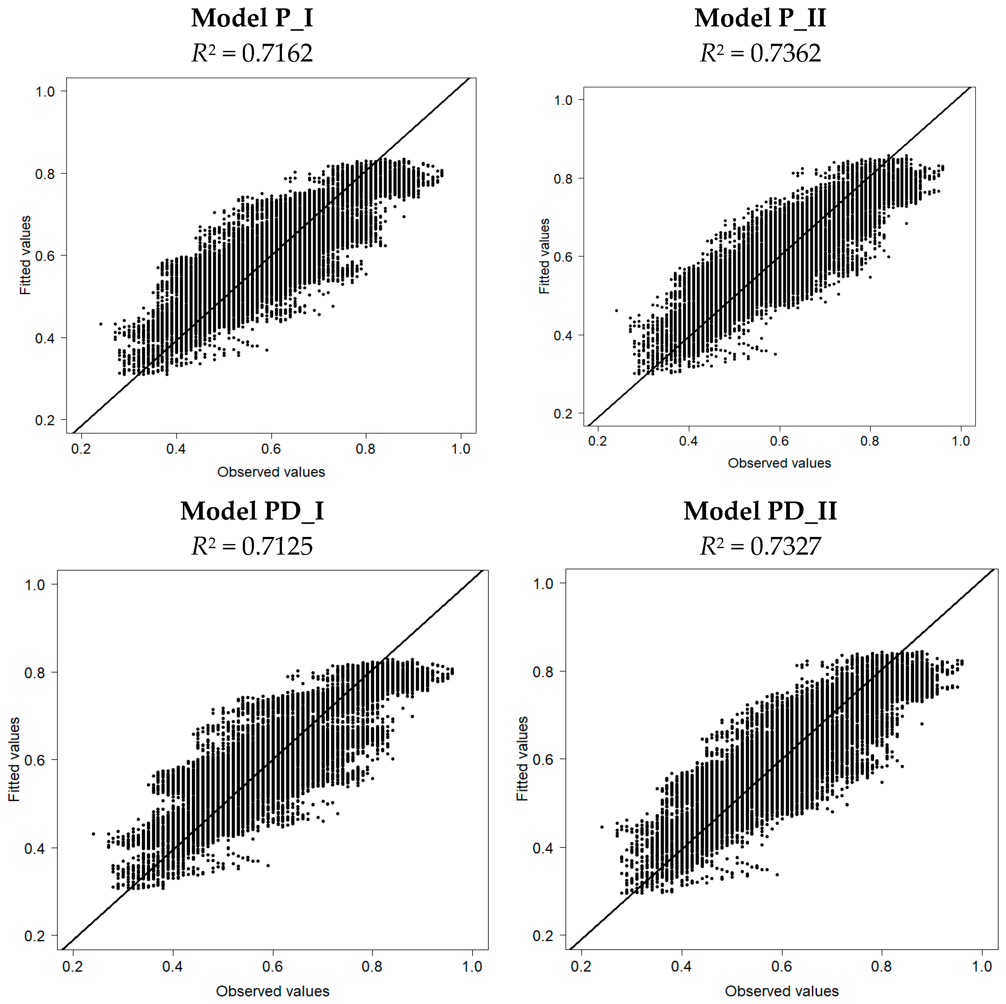
As Model PD_II provides a better fit than Model P_II, a national network manager can use it to get better predictions. However, for a more global application, Model P_II can be considered because it also presents a good goodness-of-fit between observed and fitted values.

4.4. Model Validation

One of the most critical steps in modelling is validation. To assess the predictive performance of all models considered in this study, a scatter plot of observed vs. fitted values was drawn (Figure 10). The corresponding determination coefficient (R²) suggests a good goodness-of-fit between observed and fitted values. The test of the fitted model against observed data demonstrated that both models were able to capture the variation of friction within different sections.

So, in this study, a k-fold CV method was applied to assess the prediction capacity of the Models P and PD. The 7204 sections were divided into ten (k) mutually exclusive subsets. In each iteration (k), 720 sections were used as testing data for making predictions, and 6484 sections were used as training data for parameter estimation. Once the model parameters were estimated for each training dataset, all sections from the corresponding testing dataset were used to predict the friction. Prediction errors were then calculated and subsequently used for calculating different validation statistics. The procedure was repeated ten (k) times so that each subset was used once as testing data. Mean validation statistics were then computed across the repetitions. The Root Mean Square Error (RMSE), the Mean Absolute Error (MAE), and the Mean Bias Error (MBE), which describe the average model-performance error, were examined.

Table 12. The Root Mean Square Error (RMSE), the Mean Absolute Error (MAE), the Mean Bias Error (MBE), and the respective standard deviation for each model.

Model	RMSE	(SD)	MAE	(SD)	MBE	(SD)
P_I	0.0903	(0.0002)	0.0704	(0.0001)	−0.0004	(0.0001)
P_II	0.0815	(0.0000)	0.0624	(0.0000)	−0.0005	(0.0000)
PD_I	0.0909	(0.0001)	0.0711	(0.0001)	−0.0061	(0.0002)
PD_II	0.0882	(0.0003)	0.0689	(0.0002)	−0.0060	(0.0002)

summarizes the values obtained for each model and the respective standard deviation (SD). The results show that Model II (considering the variables inherent to traffic, climate conditions, and the factors intrinsic to the highway characteristics) displays lower RMSE, MAE, and MBE. This suggests that Model II can provide better prediction accuracy than Model I (considering only the variables inherent to traffic and climate conditions).

5. Discussion and Conclusions

In this paper, four friction prediction models for flexible pavements were developed using linear mixed-effects models. Several factors influencing friction were also investigated. The random intercept models developed in this paper are an important methodological approach since they consider and correct for heterogeneity that could arise from unobserved factors not captured in the data-collection process. Moreover, the mixed-effect approach adopted was successful in identifying section-specific effects. It allowed for examining the effects of variables inherent to traffic, climate conditions, highway geometric characteristics, and type of layer.

The models showed the relevance of the geometric characteristics of the motorways, as the lane location, characteristics of plan and profile, and hypsometry, in explaining the degradation of the friction parameter through time. As far as climate, traffic, and pavement conditions are concerned, the developed models strengthen the literature review findings.

Results indicate that pavement sections’ heterogeneity may be captured through mixed-effects models and the random effect provides a more appropriate method for analyzing multi-sections pavement data. From the analysis of the signal of parameter estimates of the models, friction decreases with: Time (time), accumulated annual daily average traffic (Ac.ADT), average number of days with maximum temperature above 25 °C (average No. days temp max25), and average of total precipitation (P). It increases with the maximum air temperature value (higher max temp).

It was demonstrated that friction is also influenced by highway alignment characteristics (plan and profile), lane, type of layer, and hypsometry. Therefore, friction decreases on the right lane (RL) and the slow lane (SL), in comparison with the left lane (LL), and in the circular curve (CC) and clothoid (C) sections, in comparison with the straight alignment sections (SA), and the friction increases on the convex concordance curve (Ccv) and slope (S) in comparison with the concave concordance curve (Ccc).

Regarding the type of surface, friction decreases in the porous asphalt (PA) and gap-graded asphalt concrete with a high percentage of Rubber Modified Binder (GGA.RMB) when compared with the gap-graded asphalt concrete surface course (GGAC).

Moreover, when data on the road or highway characteristics are not available, the approach adopted is also useful. The network managers may still base their decisions on a simpler but accurate model that enables them to predict or assess the friction parameter degradation through time.

The database available for this work is limited concerning material characterization used for layers’ construction, as the Polished Stone Value (PSV), which, together with traffic, are often the main factors in friction prediction. Therefore, the models developed are restricted to pavement surfaces made of granite aggregate. In the Portuguese case, granite aggregates are used extensively on roads, and for that reason the models developed may be applied in most of the country. Besides that, in a regression model, more variation in the explanatory variables allows to more confidently pin down the relationship between the response variable and explanatory variables.

Therefore, in the future, the models developed could be upgraded using a database with surface layers made of other aggregates, whose relevant properties for friction are known. The models enable the prediction of friction degradation together with the identification of different factors that explain it, being, for these reasons, a valuable tool to assist network managers. They will be able to conduct maintenance and rehabilitation actions more efficiently, promote the best quality of the surface pavement layers, and optimize the global level of road safety. The assets management could be so much more efficient and accurate if the network manager spends extra resources to include in the database the variables inherent to the characteristics of the roads.

These models can be applied in the existing system (SUSTIMS—Sustainable Infrastructure Management System), allowing to determine the need for small to medium-term interventions and guarantee one of the crucial surface characteristics of the motorway.

References

- Chen, L.; Liu, G.; Qian, Z.; Zhang, X. Determination of allowable rutting depth based on driving safety analysis. J. Transp. Eng. Part B Pavements 2020, 146, 04020023. [Google Scholar] [CrossRef]
- European Committee for Standardization. CEN/TS 15901-7 Road and Airfield Surface Characteristics—Part 7: Procedure for Determining the Skid Resistance of a Pavement Surface Using a Device with Longitudinal Fixed Slip Ratio (LFCG): The GripTester®; CEN: Brussels, Belgium, 2009. [Google Scholar]
- Andriejauskasa, T.; Vorobjovasa, V.; Mielonas, V. Evaluation of skid resistance characteristics and measurement methods. In Proceedings of the 9th International Conference Environmental Engineering, Vilnius, Lithuania, 22–23 May 2014. [Google Scholar]
- Kassem, E.; Awed, A.; Masad, E.A.; Little, D.N. Development of predictive model for skid loss of asphalt pavements. Transp. Res. Rec. 2013, 2372, 83–96. [Google Scholar] [CrossRef]
- Wang, H.; Liang, R.Y. Predicting field performance of skid resistance of asphalt concrete pavement. In Pavement Materials, Structures and Performance, Proceedings of the Geo-Shanghai 2014 International Conference, Shanghai, China, 26–28 May 2014; Huang, B., Zhao, S., Eds.; American Society of Civil Engineers: Reston, VA, USA, 2014; pp. 296–305. [Google Scholar] [CrossRef]
- Li, Q.J.; Zhan, Y.; Yang, G.; Wang, K.C.P.; Wang, C. Panel data analysis of surface skid resistance for various pavement preventive maintenance treatments using long term pavement performance (LTPP) data. Can. J. Civ. Eng. 2017, 44, 358–366. [Google Scholar] [CrossRef]
- Pérez-Acebo, H.; Gonzalo-Orden, H.; Rojí, E. Skid resistance prediction for new two-lane roads. Proc. Inst. Civ. Eng. Transp. 2019, 172, 264–273. [Google Scholar] [CrossRef]
- Kogbara, R.B.; Masad, E.A.; Kassem, E.; Scarpas, A.T.; Anupam, K. A state-of-the-art review of parameters influencing measurement and modelling of skid resistance of asphalt pavements. Constr. Build. Mater. 2016, 114, 602–617. [Google Scholar] [CrossRef]
- Kotek, P.; Florková, Z. Comparison of the skid resistance at different asphalt pavement surfaces over time. Procedia Eng. 2014, 91, 459–463. [Google Scholar] [CrossRef]
- Kane, M.; Edmondson, V. Modelling the bitumen scour effect: Enhancement of a dynamic friction model to predict the skid resistance of rubber upon asphalt pavement surfaces subjected to wear by traffic polishing. Wear 2018, 400, 100–110. [Google Scholar] [CrossRef]
- Darabi, M.K.; Huang, C.W.; Bazzaz, M.; Masad, E.A.; Little, D.N. Characterization and validation of the nonlinear viscoelastic-viscoplastic with hardening-relaxation constitutive relationship for asphalt mixtures. Constr. Build. Mater. 2019, 216, 648–660. [Google Scholar] [CrossRef]
- Do, M.T.; Cerezo, V.; Ropert, C. Questioning the approach to predict the evolution of tire/road friction with traffic from road surface texture. Surf. Topogr. Metrol. Prop. 2020, 8, 024004. [Google Scholar] [CrossRef]
- Nicolosi, V.; D’Apuzzo, M.; Evangelisti, A. Cumulated frictional dissipated energy and pavement skid deterioration: Evaluation and correlation. Constr. Build. Mater. 2020, 263, 120020. [Google Scholar] [CrossRef]
- Viner, H.; Sinhal, R.; Parry, T. Review of UK skid resistance policy. In Proceedings of the SURF 2004: 5th Symposium on Pavement Surface Characteristics, Toronto, ON, Canada, 6–10 June 2004; p. 12. [Google Scholar]
- Kırbaş, U.; Karaşahin, M. Performance models for hot mix asphalt pavements in urban roads. Constr. Build. Mater. 2016, 116, 281–288. [Google Scholar] [CrossRef]
- West, B.; Welch, K.; Galecki, A.; Gillespie, B. Linear Mixed Models: A Practical Guide Using Statistical Software, 2nd ed.; CRC Press Taylor & Francis Group: Boca Raton, FL, USA, 2015. [Google Scholar]
- Lorino, T.; Lepert, P.; Marion, J.; Khraibani, H. Modeling the road degradation process: Nonlinear mixed effects models for correlation and heteroscedasticity of pavement longitudinal data. Procedia Soc. Behav. Sci. 2012, 48, 21–29. [Google Scholar] [CrossRef]
- Yuan, X.X.; Pandey, M.D. A nonlinear mixed-effects model for degradation data obtained from in-service inspections. Reliab. Eng. Syst. Saf. 2009, 94, 509–519. [Google Scholar] [CrossRef]
- Yu, J.; Chou, E.Y.; Luo, Z. Development of linear mixed effects models for predicting individual pavement conditions. J. Transp. Eng. 2007, 133, 347–354. [Google Scholar] [CrossRef]
- Khraibani, H.; Lorino, T.; Lepert, P.; Marion, J.M. Nonlinear mixed-effects model for the evaluation and prediction of pavement deterioration. J. Transp. Eng. 2012, 138, 149–156. [Google Scholar] [CrossRef]
- Butt, A.A.; Shahin, M.Y.; Carpenter, S.H.; Carnahan, J.V. Application of markov process to pavement management systems at network level. In Conference Summary (Third International Conference on Managing Pavements), Proceedings of the 3rd International Conference on Managing Pavements, San Antonio, TX, USA, 22–26 May 1994; Paterson, W.D.O., Connor, B.G., Eds.; National Academy Press: Washington, DC, USA, 1995; Volume 3, pp. 159–172. [Google Scholar]
- Osorio-Lird, A.; Chamorro, A.; Videla, C.; Tighe, S.; Torres-Machi, C. Application of markov chains and monte carlo simulations for developing pavement performance models for urban network management. Struct. Infrastruct. Eng. 2018, 14, 1169–1181. [Google Scholar] [CrossRef]
- Moreira, A.V.; Tinoco, J.; Oliveira, J.R.M.; Santos, A. An application of Markov chains to predict the evolution of performance indicators based on pavement historical data. Int. J. Pavement Eng. 2018, 19, 937–948. [Google Scholar] [CrossRef]
- Roberts, C.A.; Attoh-Okine, N.O. A comparative analysis of two artificial neural networks using pavement performance prediction. Comput. Aided Civ. Infrastruct. Eng. 1998, 13, 339–348. [Google Scholar] [CrossRef]
- Sanabria, N.; Valentin, V.; Bogus, S.; Zhang, G.; Kalhor, E. Comparing neural networks and ordered probit models for forecasting pavement condition in new mexico. In Proceedings of the Transportation Research Board 96th Annual Meeting, Washington, DC, USA, 8–12 January 2017. [Google Scholar]
- Mazari, M.; Rodriguez, D.D. Prediction of pavement roughness using a hybrid gene expression programming-neural network technique. J. Traffic Transp. Eng. Engl. Ed. 2016, 3, 448–455. [Google Scholar] [CrossRef]
- Marcelino, P.; Lurdes Antunes, M.; Fortunato, E.; Gomes, M.C. Machine learning for pavement friction prediction using scikit-learn. In Progress in Artificial Intelligence, Proceedings of the 18th EPIA Conference on Artificial Intelligence, EPIA 2017, Porto, Portugal, 5–18 September 2017; Oliveira, D., Gama, J., Vale, Z., Cardoso, H.L., Eds.; Springer: Cham, Switzerland, 2017; pp. 331–342. [Google Scholar] [CrossRef]
- The Portuguese Institute for Sea and Atmosphere (IPMA). Climate Normals—1971–2000. Available online: http://www.ipma.pt/en/oclima/normais.clima/1971-2000/ (accessed on 15 January 2019).
- Portal do Clima. Climate Change in Portugal. 2015. Available online: http://portaldoclima.pt/en/ (accessed on 15 January 2019).
- Anupam, K.; Srirangam, S.K.; Scarpas, A.; Kasbergen, C. Influence of temperature on tire—Pavement friction: Analyses. Transp. Res. Rec. 2013, 2369, 114–124. [Google Scholar] [CrossRef]
- JAE. MACOPAV—Manual de Concepção de Pavimentos para a Rede Rodoviária Nacional; Junta Autónoma das Estradas (JAE): Lisbon, Portugal, 1995. (In Portuguese) [Google Scholar]
- Pinheiro, J.; Bates, D.M. Mixed-Effects Models in S and S-PLUS; Springer: New York, NY, USA, 2000. [Google Scholar]
- Akaike, H. A New look at the statistical model identification. IEEE Trans. Autom. Control 1974, 19, 716–723. [Google Scholar] [CrossRef]
- Schwartz, G. Estimating the dimension of a model. Ann. Stat. 1978, 6, 461–464. [Google Scholar] [CrossRef]
- Kohavi, R. A study of cross-validation and bootstrap for accuracy estimation and model selection. Ijcai 1995, 14, 1137–1145. [Google Scholar]
- R Core Team. R. A Language and Environment for Statistical Computing; R Foundation for Statistical Computing: Vienna, Austria, 2009. [Google Scholar]
- International Business Machines Corporation (IBM Corp). IBM SPSS Statistics for Windows, Version 24; IBDM: Armonk, NY, USA, 2016. [Google Scholar]
Figure 1.
Grip Tester during a test.
Figure 2.
Number of sections for concession, highways, and districts.
Figure 3.
Friction box plot for each time period under study.
Figure 4.
Observed friction values versus time for some pavement sections.
Figure 5.
Mean profiles of friction values: (a) Versus Accumulated Annual Daily Traffic (Ac.ADT); (b) versus average No. days temp max25. Circles are observations and solid blue line is the regression line estimated by local linear regression calculation (loess).
Figure 6.
Normal quantile–quantile (Q-Q) plot of the standardized residuals from Models P_I and II.
Figure 7.
Residuals versus fitted values for Models P.
Figure 8.
Normal Q-Q plot of the standardized residuals from Models PD_I and II.
Figure 9.
Standardized residuals versus fitted values for Models PD.
Figure 10.
Observed versus fitted values of friction for the models. The line is a 1:1 line.