Abstract
Aluminizing is a common protective coating for aeroengine turbine blades, but there is no method to accurately measure the aluminized thickness. X-ray fluorescence nondestructive testing technology is a method which can basically realize the measurement of all coatings on the metal substrate. However, the aluminized coating structure is completely different from the conventional coating structure, which causes great difficulties in measuring the aluminized thickness by conventional calculation models. Therefore, to realize the measurement of aluminized thickness, a new modeling method based on radial basis function (RBF) neural network by X-ray fluorescence (XRF) is proposed. By comparing two calculation models of RBF and principal component analysis (PCA)-RBF, the results show that both models can realize the measurement of aluminized thickness, but the accuracy of PCA-RBF is better than that of RBF, and the average relative error of the predicted results is 3.99%; the predicted results of the PCA-RBF model fit the training values better, and its predictability is better.
1. Introduction
The turbine blade is an important component ensuring the safe operation of aeroengines, but it is also one of the components with the most severe working environment on aeroengines. Therefore, ensuring the safe and stable operation of turbine blades plays a crucial role in the safety and reliability of aeroengine. At present, nickel-based superalloy is a common turbine blade casting material because of its internal strengthening phase (γ′-phase) [1,2]. K403 nickel-based superalloy is a common one. However, owing to the long-term impact and erosion of high-temperature gas on turbine blades, protective measures must be performed to improve its performance in practical use [3]. Aluminizing is a common protection process, and its quality will also greatly affect the performance of turbine blades.
The uniformity of the aluminized thickness on the surface of turbine blades is one of the most important parameters affecting the performance. Nonuniform thickness will lead to nonuniform heat and stress on the turbine blades, which will cause great potential safety risks for the use of the aeroengine. The aluminized coating is composed of a variety of elements whose content constantly changes from outside to the inside, and the element types in the aluminized coating are identical to those in the substrate, which are completely different from the conventional coating structure. In a conventional coating structure, the coating and substrate are usually composed of different materials and elements. Therefore, conventional nondestructive testing methods, such as ultrasonic testing, eddy current testing, magnetic testing, and so on, are restricted by the properties of coating and substrate materials and cannot achieve the measurement of aluminized thickness [4,5]. At present, the cross-section observation method is a commonly used method for measuring the aluminized thickness of the turbine blades by scanning electron microscope, but it is a destructive method and cannot realize the comprehensive inspection of the aluminized coating on the surface. In addition, with the development of nuclear technology, the radiographic testing method is widely used in the thickness measurement of various coatings on the metal substrate, among which X-ray is most widely used [6,7,8,9,10,11]. Cao et al. [12] carried out a theoretical analysis on the thickness measurement of thin layer by X-ray fluorescence absorption method and validated the correctness of relevant theories by using experimental data. Mashin et al. [13] successfully measured the thickness of aluminum coating on steel by X-ray fluorescence. Trojek et al. [14] measured the thickness of historical materials by X-ray fluorescence, and the results showed that the measured value was in good agreement with the actual value. Giurlani et al. [15] realized the measurement of precious metal films by combining spectral acquisition of energy dispersion microanalysis with the Monte-Carlo simulation, and proposed a calculation model of secondary calibration curve. Lopes et al. [16] realized the thickness measurement of gilded layer on cultural relics by using partial least squares regression (PLS) based on X-ray fluorescence. Guilherme et al. [17] also realized the measurement of paint thickness on steel plate by means of partial least squares regression model. Wan et al. [18] designed an X-ray fluorescence thickness measurement system based on wavelet analysis, which effectively improved the accuracy of thickness measurement of sheet metal. It can be seen that the thought of nonlinear calibration and multivariate synthetic analysis has been widely applied to X-ray fluorescence thickness measurement. However, due to the special structure of aluminized coating, conventional calculation models are also not fit for the measurement of such coatings. Moreover, although the neural network model is a widely used nonlinear modeling method in the field of nondestructive testing [19,20,21,22], there is no application in the X-ray fluorescence coating thickness measurement. Therefore, based on the existing research of coating thickness measurement by X-ray fluorescence, a multivariate nonlinear model based on a neural network by X-ray fluorescence was proposed to measure the aluminized thickness in this paper.
In order to measure the thickness of aluminized coating nondestructively, the structure model was simplified according to its microstructure, firstly. Then, the samples with different thicknesses were prepared, and the X-ray fluorescence spectral data were collected. Moreover, the prediction model of the diffused aluminized layer was established by a radial basis function neural network. Finally, the accuracy of the prediction model was studied.
2. Materials and Models
2.1. Materials
The K403 nickel-based superalloy after aluminizing was used in the experiment. The K403 superalloy formed by the comprehensive strengthening of various elements was used to be the substrate. In addition, the main chemical components of K403 alloy are shown in Table 1 [23].

Table 1.
Chemical components of K403 superalloy (wt.%).
2.2. Experimental Schemes and Testing Methods
In order to realize the measurement of the aluminized thickness, the aluminized samples with different thicknesses were selected in this paper, as shown in Table 2. The thickness of each sample was calibrated by SEM (scanning electron microscope, Hitachi, Tokyo, Japan), and the size of each sample was 10 mm × 3 mm × 1 mm, as shown in Figure 1. The orange area in Figure 1 shows the position of aluminizing, and the area of X-ray fluorescence detection is within 1 mm of the cross-section of SEM observation.
Table 2.
Samples with different thicknesses and their numbers.

Figure 1.
Diagrammatic sketch of samples.
Moreover, to realize the measurement of the experimental data, the following equipment was used.
The thickness of aluminized layer was calibrated by Hitachi SU-1510 scanning electron microscope (Hitachi, Tokyo, Japan).
Fluorescence detection was operated by Elite Instruments XAU X-ray Fluorescence Coating Gauge. We selected tube voltage 25 KV, collimator Φ 0.5 mm. The measuring time of a single point was 30 s. We measured 10 times for each sample, and the fluorescence intensity of each sample was recorded as the average of the values of the 10 measurements.
2.3. Calculation Model
2.3.1. Model Simplification and Measurement Principles
The morphology and component distribution of elements along the depth of K403 superalloy after aluminizing were analyzed by means of a scanning electron microscope (SEM) (Hitachi, Tokyo, Japan) and energy dispersive spectrometer (EDS) (Oxford Instruments, Oxford, British), which were shown in Figure 2. It can be seen from Figure 2 that the morphology of the substrate is different from that of the aluminized area. Therefore, it can be considered that the substrate and coating are composed of different compounds, and the K403 superalloy after aluminizing can be simplified into the substrate–coating structure. The simplified diagram is shown in Figure 3a. The material of substrate is K403 superalloy, and the material of coating is Al alloy whose aluminum content changes continuously along depth. Here, the coating could be subdivided by the aluminum content, and the aluminized coating can be divided into countless layers of Al alloy coating with different aluminum contents. It is assumed that the thickness of each layer is x.

Figure 2.
Scanning electron microscopy (SEM) morphology and distribution of the main elements.

Figure 3.
Simplified structural model. (a) refers the simplified coating structure; (b) refers the divided layers of aluminized coating.
According to the simplified coating structure in Figure 3a and X-ray fluorescence absorption method, the calculation method of aluminized thickness can be obtained, as shown in Equation (1).
I0 represents the fluorescence intensity of the excited elements in the substrate; Id represents the fluorescence intensity received by the detector; μ represents the absorption coefficient of the coating, which is only related to the materials of coatings and the excited elements; t represents the aluminized thickness.
Based on this linear model, Giurlani et al. [15] proposed a quadratic calibration curve model. The model considered not only the absorption of coating but also the absorption of fluorescence by instruments, air, and so on, as shown in Equation (2).
Here, ,
and represent the same meanings as Equation (1); A represents the absorption coefficient caused by air, instrument and other factors; B represents the absorption coefficient of the coating.
Dividing the both sides of Equations (1) and (2) by , it could be found that the coating thickness is only related to the value of . Supposing and defining R as relative intensity, the equations could be written as Equation (3)
According to the above analysis, fluorescence is affected by many factors in the transmission process, and the absorption calibration curve cannot be a specific calculation model. Therefore, we propose a nonlinear calibration calculation model denoted by in this paper. Then, according to the simplified structure model shown in Figure 3b, the divided coatings which contain the same elements could be regarded as aluminum alloy. Therefore, we assume that the divided coatings have the same type of absorption calibration model, that is, the same type of .
Based on the above conditions, the formula for calculating the thickness of the divided coatings is shown in Equation (4)
Multiply each equation in the Equation (4) to obtain Equation (5). According to Figure 3b, due to, . Therefore, . Here, we assume , where, represents the aluminized thickness.
According to Equation (5), the aluminized thickness is only related to the value of relative intensity Therefore, the corresponding relationship between relative intensity () and aluminized thickness () could be established, and the measurement of the aluminized thickness could be realized by the law of change between them.
2.3.2. Principal Component Analysis (PCA)
Principal component analysis (PCA) was first proposed by Pearson [24] in 1901. His main point was to use mathematical transformation to recombine the input original data variables () into several “new variables” that can explain the main information of the original variables, and these “new variables” were called principal components. These principal components which are independent to each other can effectively lower the dimension of original variables and improve the modeling speed, so the accuracy of prediction results could be effectively improved [25].
Assuming the original variables have n sequences, that is, , then the principal components can be obtained by principal component analysis, which are shown in Equation (6).
are the substitution variables of the original variables, namely the principal components; is the load factor of principal component.
To realize the selection of principal components shown in Equation (6), the input data needs to be standardized, as shown in Equation (7).
where is the mean value of the observed data and is the standard deviation of . Then, the correlation coefficient matrix of the normalized independent variables, the eigenvalues of the correlation coefficient matrix and the corresponding eigenvectors of the correlation coefficient matrix are all solved. Finally, the cumulative contribution rate is calculated, as shown in Equation (8).
where represents the principal components with the largest contribution. When , these components basically reflect the overall information of the original variables. The load factor of principal component numbered m is the standard orthogonalized eigenvector of .
2.3.3. Radial Basis Function (RBF) Neural Network
Radial basis function neural network has the optimal approximation effect of arbitrary complex function and can effectively avoid the occurrence of local minimum. RBF neural network is generally composed of three layers: input layer, hidden layer and output layer. The relation diagram is shown in Figure 4.

Figure 4.
Neural network structure of radial basis function (RBF).
In Figure 4, shows the connection weight between the hidden layer and the output layer. In general, the Gaussian function is often used as the transport function in the hidden layer, as shown in Equation (9).
where, Mi represents the input value of the node numbered i in the hidden layer; Zi represents the central vector of the Gaussian function of the hidden node numbered i, which is a column vector with the same dimension as the input data; ∂ represents the normalized constant of the hidden node numbered i.
2.3.4. Experimental Data
According to the content of the main elements in the K403 superalloy shown in Table 1, the fluorescence intensity of Ni, Cr, Co, Ti and Mo were selected as the main experimental data recorded in this paper. The recorded values were the average value of the results of 10 experiments and were shown in Table 3. In the study on the calculation model of the aluminized thickness, three sets of data with the thickness of 25.1/38.1/43.2 μm were randomly selected to verify the established model, and the rest data were used to establish the calculation model.
Table 3.
Fluorescence intensity of main elements in samples with different thicknesses.
Moreover, the relative intensity (R) of the main elements was calculated and was shown in Table 4. Here, the fluorescence intensity of the sample with the thickness of 0 micron was taken as I0, which was mainly based on the following two reasons: (i) the intensity of the primary X-ray is high enough to penetrate much deeper than the aluminized thickness; (ii) the fluorescence intensity of the selected elements is also high enough to penetrate much deeper than aluminized thickness.
Table 4.
Relative intensity (R) of each element.
3. Results and Discussion
3.1. Calculation Model of Radial Basis Function (RBF) Neural Network
According to Equation (5), the aluminized thickness is only a function related to the relative intensity (R) and the aluminized thickness (t). Therefore, it is necessary to establish a mathematical model of thickness and relative intensity to achieve the accurate measurement of the aluminized thickness. In this paper, the relative intensity (R) of Ni, Cr, Co, Ti and Mo and the aluminized thickness (t) were selected to establish calculation model. A total of six observations and 30 groups of data were selected. Among them, 27 groups of data were selected as training samples and three groups of data were selected as prediction samples. The RBF neural network prediction model was established to obtain the predicted results, using the relative intensity (R) of Ni, Cr, Co, Ti and Mo as input and the aluminized thickness (t) as output.
In this paper, the newrb (P, T, goal, spread, MN, DF) function was selected as the programming basis. In this function, P and T respectively represent the input and output samples; the spread is the expansion speed of the radial basis function; the goal is the mean squared error; MN is the maximum number of neurons; DF is the number of neurons added between displays with a default value of 25. The value of spread is particularly important in this model, whose value is closely related to the change rate of the function. The larger the spread is, the smoother the approximation process will be, but the approximation error will be larger; the smaller the spread, the less smooth the approximation will be, but the approximation error of the function will be more accurate. Therefore, in the actual modeling process, the value of spread should be constantly changed so that the calculation model can achieve the best predicted results.
After repeated tests, when the spread is 0.1, the relative error of the predicted results is the smallest, and the mean square error of the training network is 0.0096, which is less than the set mean square error goal (0.01). Changing the spread again, when the mean square error is small enough and its order of magnitude reaches 10−29, the spread is 0.03. The predicted results of the above two expansion speeds are shown in Table 5.
Table 5.
Output results of the RBF neural network.
It can be seen from Table 5 that the relative error of the model changes constantly with the expansion speed change. When the expansion speed is 0.03, the mean square error of the training network is relatively low, but the average relative error reaches 67.88%, which could not meet the requirements of thickness testing. This is mainly because the expansion speed is small, which results in the non-smooth fitting process and makes it impossible to obtain the variation rule between the aluminized thickness and the relative intensity. However, with the change of the expansion speed, the mean square error of the training network increases, but the average relative error of the predicted values decreases. When the expansion speed is 0.1, the average relative error of the predicted results is 6.1%, which is the lowest and could basically meet the requirement of measurement accuracy on aluminized thickness. Under this condition, the mean square error of the training network is 0.0096, meeting the set target value 0.01. Therefore, under the condition that the set mean square error target value is met, the expansion speed is selected to be 0.1, so that the error of the predicted results meets the requirement of thickness testing.
3.2. Calculation Model of the PCA-RBF Neural Network
3.2.1. Select Variables via Principal Component Analysis
According to the steps of principal component analysis (PCA) in Section 2.3.2, principal component analysis was performed on the relative intensity (R) of Ni, Cr, Co, Ti and Mo. After calculation, two principal components were obtained, whose cumulative contribution rate was 92.65%, higher than 85%, and the relative intensity of Cr was the most influential factor. Therefore, the principal components could basically explain the information of original variables. The two principal components are shown in Equation (8).
According to Equation (8), the relative intensity of five elements in Table 4 can be converted into two principal components, as shown in Table 6.
Table 6.
The transformed principal component variables.
3.2.2. Establish PCA-RBF Calculation Model
The simplified two principal components are used as the input of the RBF neural network instead of the original five variables. Here, newrb (P, T, goal, spread, MN, DF) function was also used to establish the model in the same way as the RBF neural network model in Section 3.1. Through repeated tests, the optimal expansion speed is determined to be 0.08, and the mean square error of the training network is 3.57 × 10⁻²⁴. The predicted results of the network output are shown in Table 7.
Table 7.
The output results of the calculation model by principal component analysis (PCA)-RBF neural network.
It can be seen from that the relative error of the predicted results is 3.99% under the model of PCA-RBF, which reached a comparatively low level. The relative error under different thicknesses is also relatively stable, without fluctuating greatly.
3.3. Comparative Study on the Two Models
In order to analyze the advantages and disadvantages of the two models, this paper carries out a comparative study on the output results of the two models. Firstly, Table 8 shows the optimal mean square error of the training network and the best predicted results of the two calculation models. By comparing the effects of different expansion speeds on model performance, it is found that: (i) in the RBF model, when the mean square error of the training network is low, the error of the predicted results is high; (ii) in the PCA-RBF model, when the mean square error of the training network is the lowest, the error of the predicted results is also the lowest. Then, the relative errors of the predicted results of the two models are studied, and the results are shown in Figure 5. It can be seen from Figure 5 that the relative error of the predicted results obtained by the two calculation models is less than 10%. The relative error of the thin and thick aluminized layers is relatively high, and the relative error of the medium aluminized layer is the lowest. However, it is also clear from Figure 5 that the relative error of the PCA-RBF calculation model is more stable and will not fluctuate significantly, and the average relative error (3.99%) of all predicted results brought by the PCA-RBF calculation model is smaller than the that (6.1%) obtained by the RBF model. Finally, the change trend of the predicted results and the training values of the two calculation models is compared, as shown in Figure 6. By comparing Figure 6a with Figure 6b, it can be seen: (i) under the RBF neural network model, the predicted results and the training values vary with the relative intensity (R) in a disorderly manner, and there is no obvious uniform trend; (ii) under the PCA-RBF neural network model, the predicted results and the training values are basically consistent with the change trend of the two principal component variables, and the change curve of the predicted results basically fits in the training values.
Table 8.
The best mean square error and predicted results.
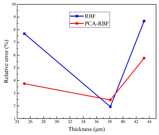
Figure 5.
Relative error of the two models.
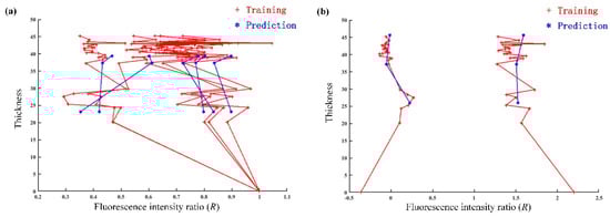
Figure 6.
The changing trend of training values and predicted values ((a) refers to the RBF model; (b) refers to the PCA-RBF model).
In conclusion, the PCA-RBF neural network model can not only obtain high accuracy, but also fit into the training network well. Therefore, when solving practical problems, the performance of the PCA-RBF neural network model is better than that of the RBF neural network, and it is more suitable for the measurement of aluminized thickness.
4. Conclusions
By the X-ray fluorescence nondestructive testing method, a new nonlinear modeling method of coating thickness measurement based on radial basis function neural network was proposed in this paper. Additionally, by comparing the results of RBF and PCA-RBF neural network calculation model, the results show:
- (1)
- Both RBF and PCA-RBF models can realize the measurement of the aluminized thickness under suitable expansion speed. The optimal average relative error of the predicted results is 6.1% and 3.99% respectively, which shows that the PCA-RBF model can obtain better predicted results in the calculation of aluminized thickness.
- (2)
- The relative error of the predicted results of different aluminized thicknesses displayed by the PCA-RBF model is more uniform and does not fluctuate greatly, which means that PCA-RBF model has better stability.
- (3)
- The change rule of the predicted results in the PCA-RBF model is more significantly consistent with the change rule of the training values, and the PCA-RBF model can better reflect the change rule of the aluminized thickness with the relative intensity.
To sum up, after data preprocessing, the calculation accuracy of the model can be improved effectively. Moreover, the new nonlinear modeling method proposed in this paper better realized the measurement of aluminized thickness, which provides a new idea for measuring the coating thickness of non-conventional structures. However, as far as the data sizes are concerned, the data sizes selected in this paper are still limited, and more data should be prepared in the future. With an increase in data size, the accuracy of the predicted results and the stability of the model are expected to be further improved.
Author Contributions
Writing–original draft, J.L.; writing–review & editing, C.W.; methodology, P.Z.; resources, M.G.; funding acquisition, L.T.; data curation, B.L. All authors have read and agreed to the published version of the manuscript.
Funding
This study was supported by Research Fund of Department of Basic Sciences at Air Force Engineering University (No. JK2020202).
Conflicts of Interest
No potential conflict of interest was reported by the authors.
References
- Heilmaier, M.; Leetz, U.; Reppich, R. Order strengthening in the cast nickel-based superalloy IN 100 at room temperature. Mater. Sci. Eng. 2011, A319–321, 375–378. [Google Scholar] [CrossRef]
- Miller, M.K. Contributions of atom probe tomography to the understanding of nickel-based superalloys. Micron 2011, 32, 757–764. [Google Scholar] [CrossRef]
- Xie, M.Y.; Wang, C.; Zhang, P.Y.; Chai, Y.; Dai, P.L.; Li, Q.L. Effects of composite strengthening on microstructure and mechanical property of K403 aluminized alloy. Chin. Surf. Eng. 2018, 31, 26–31. [Google Scholar]
- Ji, A. Development of X-ray fluorescence spectrometry in the 30 years. Rock Miner. Anal. 2012, 31, 383–398. [Google Scholar]
- Dwivedi, S.K.; Vishwakarma, M.; Soni, A. Advances and researches on nondestructive testing: A review. Mater. Today Proc. 2018, 5, 3690–3698. [Google Scholar] [CrossRef]
- Jain, S.K.; Gupta, P.P.; Rao, S.M. XRF technique for the measurement of nickel coating thickness in the range of a few hundred angstroms. In Proceedings of the Material Science Symposium, Rourkela, India, 24–26 October 1977. [Google Scholar]
- Kataoka, Y.; Kohno, H.; Furusawa, E.; Mantler, M. XRF analysis of Zn–Fe alloy coatings by using measurements at two take-off angles. X-Ray Spectrom. 2007, 36, 221–225. [Google Scholar] [CrossRef]
- Fiorini, C.; Gianoncelli, A.; Longoni, A.; Zaraga, F. Determination of the thickness of coatings by means of a new XRF spectrometer. X-Ray Spectrom. 2002, 31, 92–99. [Google Scholar] [CrossRef]
- Nygard, K.; Hamalainen, K.; Manninen, S.; Jalas, P.; Ruottinen, J.P. Quantitative thickness determination using x-ray fluorescence: Application to multiple layers. X-Ray Spectrom. 2004, 33, 354–359. [Google Scholar] [CrossRef]
- Al-Merey, R.; Karajou, J.; Issa, H. X-ray fluorescence analysis of geological samples: Exploring the effect of sample thickness on the accuracy of results. Appl. Radiat. Isot. 2005, 62, 501–508. [Google Scholar] [CrossRef]
- Rolin, T.D.; Leszczuk, Y. X-ray Fluorescence Spectroscopy Study of Coating Thickness and Base Metal Composition; NASA: Washington, DC, USA, 2008. [Google Scholar]
- Cao, L.G.; Ding, Y.M.; Ao, Q. Thin-layer thickness gauging based on X-ray flourecence absorption method. Nucl. Tech. 1989, 12, 580–586. [Google Scholar]
- Mashin, N.I.; Leont’eva, A.A.; Tumanova, A.N. X-ray fluorescence method for determining the thickness of an aluminum coating on steel. J. Appl. Spectrosc. 2011, 78, 427–432. [Google Scholar] [CrossRef]
- Trojek, T.; Musílek, L.; Prokeš, R. Depth of layers in historical materials measurable by X-ray fluorescence analysis. Radiat. Phys. Chem. 2019, 155, 239–243. [Google Scholar] [CrossRef]
- Giurlani, W.; Innocenti, M.; Lavacchi, A. X-ray Microanalysis of Precious Metal Thin Films: Thickness and Composition Determination. Coatings 2018, 8, 1–12. [Google Scholar] [CrossRef]
- Lopes, F.; Melquiades, F.L.; Appoloni, C.R.; Rizzutto, M.A.; Silva, T.F. Thickness determination of gold layer on pre-Columbian objects and a gilding frame, combining XRF and PLS regression. X-Ray Spectrom. 2016, 45, 344–351. [Google Scholar] [CrossRef]
- Guilherme, A.; Lisboa, N.; Paulo, S.P.; Dos Santos, F.R.; Luiz Melquiades, F. Determination of metal content in industrial powder ink and paint thickness over steel plates using X-Ray Fluorescence. Appl. Radiat. Isot. 2019, 150, 168–174. [Google Scholar]
- Wan, C.Y.; Hou, F.; Zhou, K.; Wang, J.C.; Tao, J.; Zhang, H.F.; Feng, D.R. Design of high precision X-ray thickness gauge system based on wavelet analysis. Ind. Instrum. Autom. 2019, 3, 113–117. [Google Scholar]
- Liu, B.; Li, A.H.; Wang, C.L.; Wang, J.B.; Ni, Y.T. SOM and RBF Networks for Eddy Current Nondestructive Testing. Adv. Mater. Res. 2011, 219–220, 1093–1096. [Google Scholar] [CrossRef]
- Sun, X.Y.; Liu, D.H.; Li, A.H. The Use of RBF Based on Fisher Ratio for Eddy Current Nondestructive Detecting System. In Proceedings of the Third International Conference on Natural Computation, Haikou, China, 24–27 August 2007; Volume 1, pp. 334–337. [Google Scholar]
- Thatoi, D.; Guru, P.; Jena, P.K.; Choudhury, S.; Chandra Das, H. Comparison of CFBP, FFBP, and RBF Networks in the Field of Crack Detection. Model. Simul. Eng. 2014, 1–3. [Google Scholar] [CrossRef]
- Su, L.; Shi, T.L.; Liu, Z.P.; Zhou, H.D.; Du, L.; Liao, G.L. Nondestructive diagnosis of flip chips based on vibration analysis using PCA-RBF. Mech. Syst. Signal Process. 2017, 85, 849–856. [Google Scholar] [CrossRef]
- Editorial board of china aviation materials handbook. China Aviation Materials Handbook, 2nd ed.; Standards Press of China: Beijing, China, 2002; p. 9. [Google Scholar]
- Pearson, K. Principal components analysis. Edinb. Dublin Philos. Mag. J. 1901, 6, 566. [Google Scholar]
- Gao, X.P.; Chen, L.L.; Liu, Y.Z.; Sun, B.W. PCA-RBF neural network model-based urban water consumption prediction. Water Resour. Hydropower Eng. 2017, 48, 1–6. [Google Scholar]


© 2020 by the authors. Licensee MDPI, Basel, Switzerland. This article is an open access article distributed under the terms and conditions of the Creative Commons Attribution (CC BY) license (http://creativecommons.org/licenses/by/4.0/).