CFD Simulation and Optimisation of a Low Energy Ventilation and Cooling System

John Kaiser Calautit; Dominic O'Connor; Polytimi Sofotasiou; Ben Richard Hughes

doi:10.3390/computation3020128

,

and

Department of Mechanical Engineering, University of Sheffield, Sheffield S10 2TN, UK

^*

Author to whom correspondence should be addressed.

^†

These authors contributed equally to this work.

Computation2015, 3(2), 128-149;https://doi.org/10.3390/computation3020128

This article belongs to the Special Issue Computational Fluid Dynamics in Civil Engineering

Version Notes

Order Reprints

Abstract

Mechanical Heating Ventilation and Air-Conditioning (HVAC) systems account for 60% of the total energy consumption of buildings. As a sector, buildings contributes about 40% of the total global energy demand. By using passive technology coupled with natural ventilation from wind towers, significant amounts of energy can be saved, reducing the emissions of greenhouse gases. In this study, the development of Computational Fluid Dynamics (CFD) analysis in aiding the development of wind towers was explored. Initial concepts of simple wind tower mechanics to detailed design of wind towers which integrate modifications specifically to improve the efficiency of wind towers were detailed. From this, using CFD analysis, heat transfer devices were integrated into a wind tower to provide cooling for incoming air, thus negating the reliance on mechanical HVAC systems. A commercial CFD code Fluent was used in this study to simulate the airflow inside the wind tower model with the heat transfer devices. Scaled wind tunnel testing was used to validate the computational model. The airflow supply velocity was measured and compared with the numerical results and good correlation was observed. Additionally, the spacing between the heat transfer devices was varied to optimise the performance. The technology presented here is subject to a patent application (PCT/GB2014/052263).

Keywords:

hot climates; indoor air; natural ventilation; passive cooling; sustainable

1. Introduction

Commercial wind towers are passive ventilation systems adapted from vernacular architecture of Middle Eastern cultures that date back hundreds of years [1]. Wind towers are capable of delivering ventilation to buildings by the manipulation of pressure differences caused by wind velocity and buoyancy effects of thermally stratified air. Mechanical Heating Ventilation and Air-Conditioning (HVAC) systems commonly used to ventilate and condition air for buildings account for 60% of the total energy consumption in the operation and maintenance of buildings [2]. As a sector, the construction, operation and maintenance of buildings contributes 40% of the total global energy demand [3]. By using new technology coupled with passive ventilation from wind towers, significant amounts of energy can be saved, reducing the emissions of greenhouse gases.

The development of commercial wind towers can be seen to run parallel to the development of Computational Fluid Dynamics (CFD). As improvements in the commercial codes capable of being processed and advancements in mesh detail have pushed CFD analysis forward, the computing power capable in CFD analysis had resulted in the design of commercial wind towers in more efficient and compacts approaches capable of meeting recommended guideline levels of ventilation without causing significant architectural provocations. Early work in fluid analysis was completed by hand calculation, resulting in slow progress and long calculation time with only very simple and small grids being analysed. Early analysis of natural ventilation did not espouse the use of CFD, instead relying on numerical methods to provide guidance for design [4].

More recently, CFD analysis had become vital to design engineers and researchers interested in obtaining fast and accurate data, used to inform design decisions for prototype technology. This was equally true for those interested in commercial wind towers [5]. The speed at which modifications can be introduced and tested in design through the use of CFD far outstrips the practicality of experimental testing though it should be noted that both methods of analysis complement each other for complete validation of a design [6].

In this study, the development of CFD analysis in aiding the development of wind towers was explored. Initial concepts of simple wind tower mechanics to detailed design of wind towers which integrate modifications specifically to improve the efficiency of wind towers were detailed. From this, using CFD analysis, heat transfer devices were integrated into a wind tower to provide cooling for incoming air, thus negating the reliance on mechanical HVAC systems. Furthermore, the spacing between the heat transfer devices was varied to optimise the cooling and natural ventilation performance.

2. Previous Related Work

2.1. CFD Simulation of Wind Towers

Wind towers provide passive ventilation of buildings by supplying external air and extracting indoor air by manipulating pressure differences around buildings. Areas of positive pressure are created on the windward faces of objects as wind velocity increases, areas of negative pressure are created on the leeward faces. This difference in pressure causes the movement of air from the areas of positive pressure to the areas of negative pressure to attempt to equalise the pressure. This is one of the principles which wind towers are able to manipulate to provide ventilation to buildings. Negative pressure on the leeward faces of the wind tower create suction forces, drawing air out of the building, this is replaced by air from the windward faces of the wind tower forced through by the positive pressure. This is shown schematically in Figure 1.

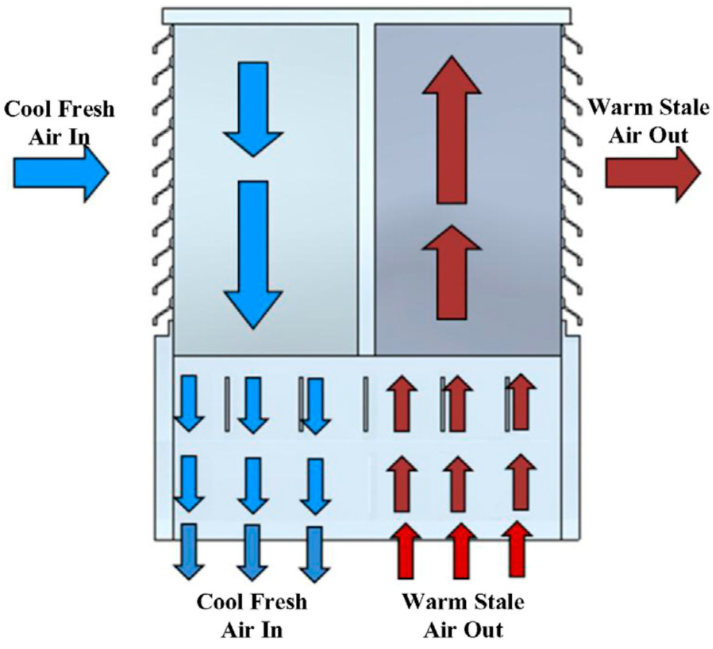
Figure 1. Schematic of typical wind tower operation.

Wind towers also operate by a secondary action of the stack effect; the density of air decreases as the temperature increases, causing warmer air to rise. The warm air is passes through the wind tower and escapes to the environment. Cooler, fresh air replaces the outgoing air, either through the wind tower or open doors and windows lower in the structure. Linden [7] provided comprehensive models of the fluid flow involved in natural and passive ventilation, much of the work completed helped with the development of CFD analysis for wind towers.

Prior to the development of modern commercial wind towers, Bahadori [8] investigated traditional wind towers. The aim of this was to better understand the operation and ventilation techniques of traditional wind towers and determine if modifications could be made. The aims of the modifications were to reduce the dust infiltration into the building through the wind tower and provide cooling of the incoming air to improve thermal comfort to occupants. Following the design modifications proposed by Bahadori, it was found that the flow rate through the wind tower increased whilst the dust infiltration was reduced. Furthermore, the ability of the wind tower to cool the incoming air was significant when evaporative cooling sprinklers were integrated into the design. Yaghoubi et al. [9] provided similar analysis which aligned with the measurements and conclusion drawn by Bahadori.

Computational Fluid Dynamics (CFD) analysis provided designers and engineers with a quicker method of processing modifications to wind towers than numerical methods allow. In addition to this, dependence on long and expensive experimental testing can be minimised to a stage when final modifications had been agreed upon. The advancements in processing power of work stations had resulted in greater detail in results due to increased mesh quality and better reliability due to the number of models commercial CFD codes were capable of running depending on the conditions required.

CFD had been used by a wide range of researchers interested in the analysis and design of wind towers. Hughes and Mak [10] compared the efficiency of the two primary methods of ventilation through wind towers; wind driven flow and buoyancy driven flow. A model of a wind tower integrated into a building to provide ventilation air was designed, air flow could be provided by a velocity inlet boundary condition or by heating of the internal building air to create density stratification. The results from the CFD analysis showed that wind driven air flow was able to provide 76% more supply air than the buoyancy effect. A flow visualisation of the wind driven flow can be seen in Figure 2a.

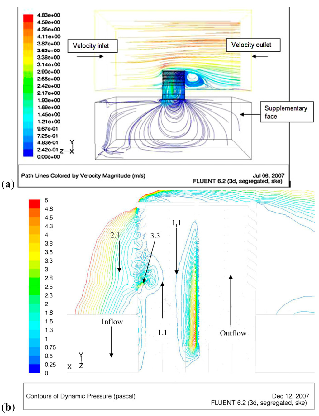
Figure 2. (a) Velocity vectors simulating the con-current flow through the wind tower [10]; (b) Computational Fluid Dynamics (CFD) calculated pressure contours at louvre angle of 35° [11].

Due to the ability to change dimensions and design quickly through the use of computer-aided design (CAD) programs which integrated into CFD simulations, on the fly modifications was made to concepts. This approach had been readily employed in the development of wind towers. A large section of the research that had been conducted in relation to the development of wind towers was to improve the air velocity through the wind tower and provide the maximum amount of supply air. Liu et al. [12] focused on determining the optimum length and number of louvers in a wind tower. Louvers were used on wind towers to accelerate air flow through the wind tower whilst also preventing the ingress of unwanted particles such as pollution, rain and snow. By increasing the number of louvers on the wind tower, it was found that the flow through the wind tower increased. A 12.7% increase in air flow rate was observed by the addition of 2–3 louvers to a maximum total number of 6–8 louvers. Beyond this number of louvers the air flow rate only increased by 1.5%. Furthermore, short-circuiting, air entering and exiting the wind tower without circulating around the building, was observed in the upper section of the wind tower due to the high number of louvers.

In addition to increased number of louvers used in the study, the length of the louvers protruding from the wind tower was altered. It was also noted that a single louver length for wind towers of varying sizes would not be sufficient due to the likeliness of varying performance. Therefore a length ratio was applied l = L/L_ref. L is the nominal length of the louver and L_ref is the louvers length when the dimension of louver projection on the corresponding quadrant equates with the gap between two adjacent louvers, L_gap. Results from simulations showed that the optimum value for louver length is when the length ratio is close to 1. The performance of the wind tower for ventilation is influenced by the louver length.

As the design of louvers was a critical factor in the efficiency of wind towers, Hughes and Ghani [11] conducted a similar study. The angle of the louvers was varied by increments of 5° within a range of 10°–45°. This was done to analyse the effect on the air flow rate and pressure distribution within the building. It was established that the maximum internal air velocities were measured at a louver angle of 35°. Above 35°, flow separation occurs at the louvers reducing the ventilation rate of the wind tower. A pressure contour plot can be seen in Figure 2b for the louver angle designed at 35°.

The geometry of a wind towers was a significant factor in the overall performance for ventilation. The majority of analysis of wind towers was conducted using a square or rectangular shape with flat surfaces and sharp edges. Multi-direction wind towers were tested by Montazeri [13] to determine the effect of increasing the number of internal section within the wind tower on the behaviour of the air flow. Five different shapes of wind towers were tested experimentally in a wind tunnel and validated by numerical modelling. Two sided, three sided, four sided, six sided and twelve sided variations were all tested by measuring the air flow rate into a test room at different air incident angles [13].

This research was driven by the understanding that for a typical square four sided wind tower, maximum efficiency was possible at a wind incident angle of 45°. In addition to this, a large portion of a four sided wind tower was used to extract internal air; Montazeri proposed that a more appropriate use of sections of the wind tower would be for supply; this was tested using a circular cross section for the wind tower with increasing number of divisions. Experimental testing and numerical modelling proved this idea to be incorrect; a rectangular wind tower was 13% more efficient than a circular design. Furthermore, at an incident angle of 0° increasing the number of partitions within the wind tower decreased the induced air flow rate within the test room. However, as the number of partitions was increased the influence of a changing incident angle of the air flow was reduced.

2.2. CFD Simulation of Heat Transfer Devices

Despite the innovations that had been accomplished through the use of CFD for the development of wind towers, regulating the temperature of supply air through a low energy process still remains incomplete. Heat transfer devices technology could provide the link between passive ventilation and low energy temperature regulation [14]. It had been noted previously that heat transfer devices integrated into other ventilation systems do not create a significant pressure drop compared to other technology, this was critical in the integration into passive ventilation systems as pressure losses should be kept to a minimum. Gan and Riffat [15] conducted CFD analysis to understand the causes of pressure loss within a heat recovery system with heat transfer devices. It was found that pressure loss was a result of the blockage caused by the physical presence of the heat transfer devices; which was further increased by the addition of fins and smaller spacing. An indirect cause of pressure loss came from the reduced temperature difference between the supply and exhaust air streams after the heat recovery.

Hughes et al. [16] completed CFD modelling to determine the most effective arrangement of heat transfer devices to allow air streams to flow through. Both the pitch and distance between heat transfer devices were varied along with the horizontal or vertical arrangement in order to determine which arrangement resulted in the greatest heat recovery (Figure 3). The optimal arrangement of heat transfer devices was determined as a pitch of 0.035 m between centres, pre-cooling recovery was calculated at 15.6 °C in hot, dry climates. Pre-heating was calculated at 3.3 °C across the heat transfer devices for a milder climate. Calautit et al. [17] used a similar CFD methodology when modelling heat transfer devices in a vertical and horizontal arrangement. This analysis yielded similar results in terms of temperature drop.

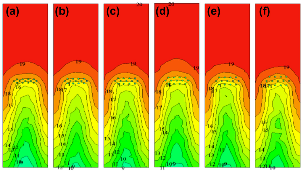
Figure 3. Effect of different pitch spacing on the temperature profile (a) 0.020 m (b) 0.025 m (c) 0.030 m (d) 0.035 m (e) 0.040 m (f) 0.045 m [16].

2.3. CFD Optimisation of Natural Ventilation Systems

Due to demanding need for holistic ventilation design approaches, researchers employed optimization techniques, leading to optimal or improved design solutions. Stavrakakis et al. [18] employed CFD techniques to investigate the most reliable turbulence model for the study of naturally cross-ventilated building model. In sequence, for the same model, Stavrakakis et al. [19] performed coupled CFD-Artificial Neutral Network (ANN) techniques to evaluate the effect of different opening configurations and building directions on the ventilation rate, minimizing simultaneously the percentage of dissatisfaction. Similar simulation-based optimization techniques were employed by Zhou and Haghighat [20], who investigated the result of various influential parameters, such as temperature, airflow, position and number of ventilation systems, etc., in an office environment, in order to determine the most energy efficient ventilation systems configuration for optimal comfort conditions.

Shen et al. [21] employed Response Surface Methodology (RSM) techniques to investigate the impact effect of the wind speed and direction on the ventilation rate of a naturally ventilated building. They examined several Design of Experiments (DoE) methods to determine the quadratic response surface that shows better performance on the prediction of ventilation rate. In a more recent work, Shen et al. [22] employed similar RSM techniques to study the ventilation efficiency on a livestock building, under variable window opening sizes and outdoor wind conditions. The results obtained from CFD simulations revealed that the Box-Bohnken Design (BBD) and Central Composite Rotation Design (CCRD) methods can accurately predict the response behavior. However, the performance of the selected DoE methods may vary depending on the case study.

CFD techniques were also used for conducting parametric studies, intending to identify design solutions that would achieve increased ventilation rates, improving comfort conditions. Lal [23] studied different geometrical characteristics for a solar chimney integrated into a building structure. CFD simulations enabled the identification of an enhanced chimney design, reducing the internal temperature up to 4 °C. Calautit et al. [24] determined the spacing and arrangement for wind towers for optimum natural ventilation performance.

Yin et al. [25] evaluated 16 CFD models of different ventilation scenarios and exhaust location, in a patient ward. The simulation study revealed that the location of the exhaust, depending on the ventilation system (displacement or mixing), was of great importance in the air quality and contaminant dispersion. Aliabadi et al. [26] used CFD to design and optimise the performance of a hybrid ventilation scheme for a dining hall. The influence of occupancy, heating and cooling modes, ceiling fans operation low level bypass exhaust on the ventilation energy consumption and thermal comfort were investigated.

3. CFD Methodology

A commercial general purpose CFD code ANSYS FLUENT was used in this study to simulate the airflow inside the wind tower model and into to the small room connected to it. The simulation was conducted at steady state and with a three-dimensional computational domain. The CFD code uses the Finite Volume Method (FVM) with the Semi Implicit Method for Pressure Linked Equations (SIMPLE) velocity-pressure coupling algorithm. The Finite Volume Method (FVM) is a discretisation technique for solving partial differential equations that computes the values of the conserved variables averaged across a domain. The first step was to subdivide the domain into a number of elements. At the centroid of each of the elements, the variable values were computed. The next step was to transform the governing partial differential equations in a conservative form and solved over discrete elements. The resulting equation is called the discretised equation. As the effect of heat transfer across the heat pipes was of high importance in this study, the SIMPLE algorithm was chosen. Furthermore, the as wind driven flow was the dominant driving force for airflow, SIMPLE was deemed the most appropriate solution [27]. The turbulent component of the airflow was modeled using the k-epsilon turbulence model [28,29]. The governing equations for the mass conservation (Equation (1)), momentum conservation (Equation (2)), energy conservation (Equation (3)), turbulent kinetic energy (Equation (4)), and energy dissipation rate (Equation (5)) are detailed below:

\frac{\partial ρ}{\partial t} + \nabla \times (ρ u) = 0

(1)

where ρ is density, t is time and u refers to fluid velocity vector.

\frac{\partial (ρ u)}{\partial t} + \nabla \times (ρ u u) = - \nabla p + ρ g + \nabla \times (μ \nabla u) - \nabla \times τ_{t}

(2)

where p is the pressure, g is vector of gravitational acceleration, μ is molecular dynamic viscosity and τ_t is the divergence of the turbulence stresses which accounts for auxiliary stresses due to velocity fluctuations.

\frac{\partial (ρ e)}{\partial t} + \nabla \times (ρ e u) = \nabla \times (k_{e f f} \nabla T) - \nabla \times (\sum_{i} h_{i} j_{i})

(3)

where e is the specific internal energy, k_eff is the effective heat conductivity, T is the air temperature, h_i is the specific enthalpy of fluid and j_i is the mass flux.

\frac{\partial (ρ k)}{\partial t} + \nabla \times (ρ k u) = \nabla \times [a_{k} μ_{e f f} \nabla k] + G_{k} + G_{b} - ρ_{ε}

(4)

\frac{\partial (ρε)}{\partial t} + \nabla \times (ρε u) = \nabla \times [a_{ε} μ_{e f f} \nabla ε] + C_{1 ε} \frac{ε}{k} (G_{k} + C_{3 ε} G_{b}) - C_{2 ε} ρ \frac{ε^{2}}{k}

(5)

where G_k stands for source of turbulent kinetic energy due to average velocity gradient, G_b is source of turbulent kinetic energy due to buoyancy force, α_k and α_ε are turbulent Prandtls numbers, C_1ε, C_2ε and C_3ε, are empirical model constants.

3.1. Design Geometry

The wind tower geometry (Figure 4a) was created using Solid Edge CAD software and then imported into ANSYS Geometry (FLUENT pre-processor) to create a computational model. The solid parts of the wind tower and test room geometry were created using the CAD software. However, replicating the physical geometry of the wind tower does not represent a computational domain. To achieve this, the fluid volume was defined before generating a computational mesh. The fluid volume was extracted from the solid model as shown in Figure 5a. The fluid volume or domain was separated into three parts: the macro-climate (external), wind tower and micro-climate (test room). The macro-climate was created to simulate the airflow around the wind tower model. The macro-climate consisted of an inlet at the left hand side of the domain, and an outlet on the opposing boundary wall of the macro climate. The distance between the wind tower and the wall of the macro-climate was determined by calculating the blockage caused by the wind tower model. The macro-climate dimensions was 5 m × 5 m × 10 m. According to the dimensions of the wind tower (1 m × 1 m × 1 m), the model produced a maximum blockage of 4.8%, therefore no corrections were made to the measurements obtained with these configurations [13].

The wind tower device was incorporated to a micro-climate with the height, width, and length of 3 m × 5 m and 5 m, representing a small room [30,31]. The wind tower was modelled with seven louvres angled at 45° [11]. The wind tower was assumed to be supplying at 100% (fully open), therefore the volume control dampers was not added to the model [30]. The cylindrical heat transfer devices, each with an outer diameter of 0.02 m, were integrated in to the lower part of the wind tower channel. Figure 4b illustrates the arrangement of the heat transfer devices inside the wind tower. In order to determine the optimum cooling and ventilation performance of the wind tower, the horizontal spacing of the heat transfer devices were varied. The horizontal spacing (x) between the heat transfer devices was varied between 50 mm and 100 mm.

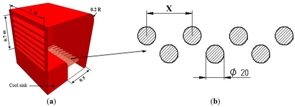
Figure 4. (a) Illustration of the computer-aided design (CAD) geometry of the wind tower with heat transfer devices; (b) Cross-sectional diagram of the heat transfer device in staggered arrangement.

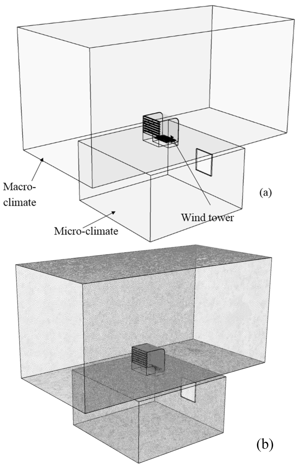
Figure 5. (a) Illustration of the geometry; (b) Meshing of the macro-climate, wind tower and test room.

3.2. Mesh Generation and Verification

Due to the geometrical complexity, an unstructured mesh was used to discretise the surface and volumes of the computational domains [32]. To be able to capture properly the flow fields near the critical areas of interest in the simulation such as the heat transfer devices and louvers, size functions were applied in those surfaces. The size of the mesh element was extended smoothly to resolve the sections with high gradient mesh and to improve the accuracy of the results of the velocity and temperature fields [33]. The mesh element size was varied from 0.005 m for the mesh near the heat transfer devices and louvers to 0.07 m for the middle of the space. Figure 5b shows the meshing of the modeled wind tower and room using ANSYS Mesh. The total number of the mesh elements used for the CFD analysis was equal to 7,249,235.

Mesh verification method was used to validate the programming and computational operation of the model. The numerical grid was refined and locally enriched using the h-method grid verification. The h-method (mesh refinement) refers to the targeting of areas of the mesh which have high levels of skewness and replacing them with an increased number of elements, or a different element type. The mesh was evaluated and refined until the posterior estimate error becomes insignificant between the number of elements and the posterior error indicator [33,34].

The mesh verification method starts with a coarse mesh and gradually refines it until the variation observed between the results were smaller than the predefined acceptable error. The accuracy of the results was improved by using successively smaller cell sizes for the computation [33,35]. The set boundary conditions remained fixed throughout the simulation process to ascertain precise comparison of the results. The initial coarse grid consisted of 2,674,484 elements which was refined over five stages until an acceptable error of 0.01% was achieved with a total of 7,249,235 elements.

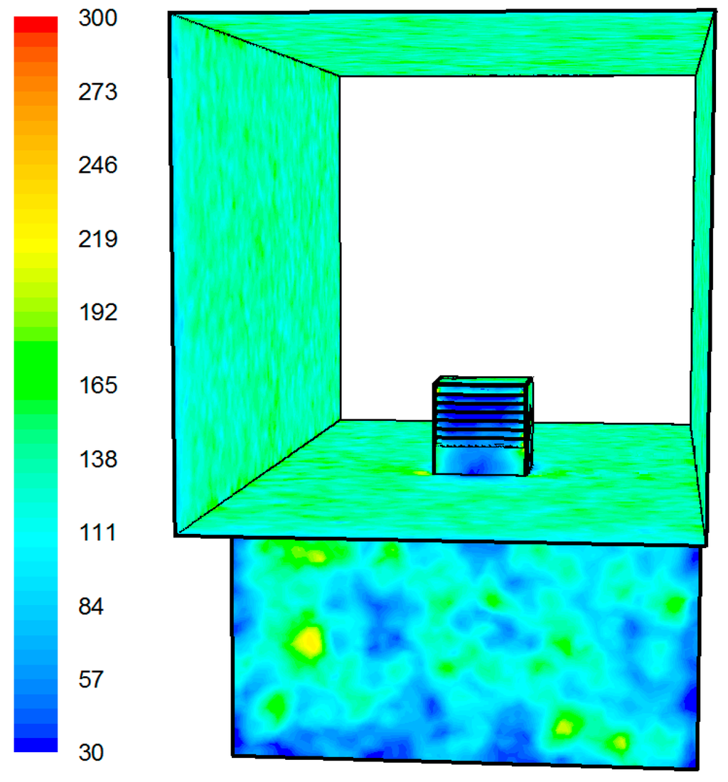
Figure 6. Contour of wall y-plus value.

Furthermore, the grid resolution was determined taking into account an acceptable value for the wall y+. The log-law, which is valid for equilibrium boundary layers and fully developed flows, provides upper and lower limits of the acceptable distance between the near-wall cell centroid and the wall. The distance is usually measured in the dimensionless wall units, y+. For standard wall functions, each wall-adjacent cell’s centroid should be located within the log-law layer, 30 < y+ < 300 [28]. Figure 6 shows the wall y+ analysis for the model.

3.3. Boundary Conditions

Figure 7 shows the physical domain containing the macro- and micro-climate fluid volumes. A wall boundary condition was used to create a boundary between each region. The macro-climate fluid volume, used to simulate the external velocity of the flow field, generated velocity into the wind tower. A horizontal plane was used as a velocity inlet, while the opposite boundary wall was set as the pressure outlet (atmospheric). The velocity inlet was varied between 0 and 5 m/s. The external air temperature was set to 318 K to simulate a hot external environment. The external air temperature was also varied between 318 K and 302 K. In order to cool the air that was supplied to the room, the surface temperature of the heat transfer devices was set to 293 K. An opening located at the leeward side of the room was set as pressure outlet (atmospheric) to extract the air out of the room. The influence of the internal gains (occupants, equipment, etc.) and heat gain through walls were not investigated in this work.

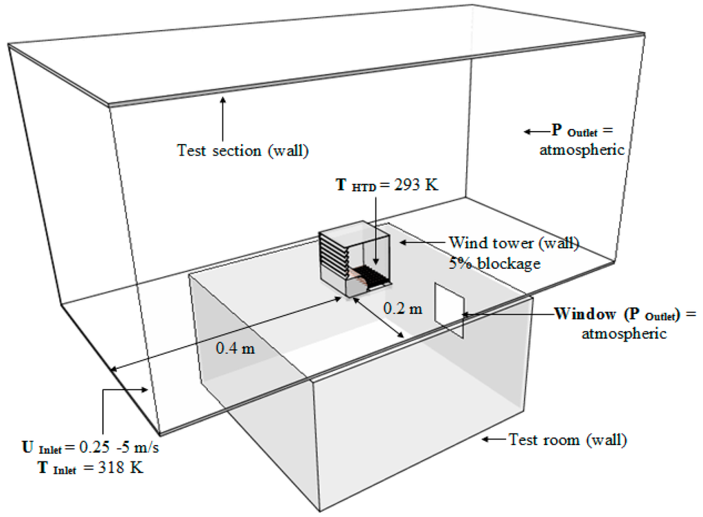
Figure 7. Flow domain of the computational model showing the boundary conditions.

3.4. Solution Convergence

Solution convergence is the term for a numerical method using iterations to produce a solution of the grid, whereby the error approaches zero. Solutions are based on iterations against pre-defined convergence criterion [28]. The default convergence criterion in FLUENT is 10-6 for the energy equation and 10-3 for all other equations. When the set convergence criterion is met the iteration process is complete. In this study, the convergence checking was disabled and the convergence was monitored by examining the residual levels (Figure 8). In addition, relevant integrated quantities such as the indoor and supply air velocity (Figure 9) and temperature (Figure 10) were also monitored.

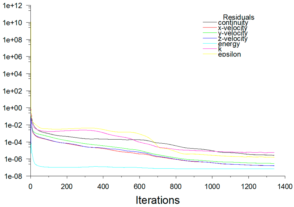
Figure 8. CFD solution residuals.

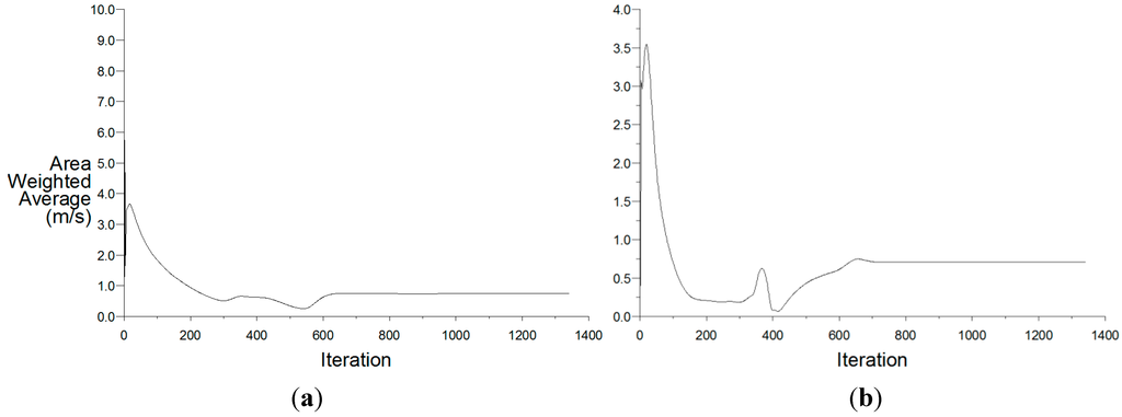
Figure 9. (a) Indoor velocity; and (b) air supply velocity convergence.

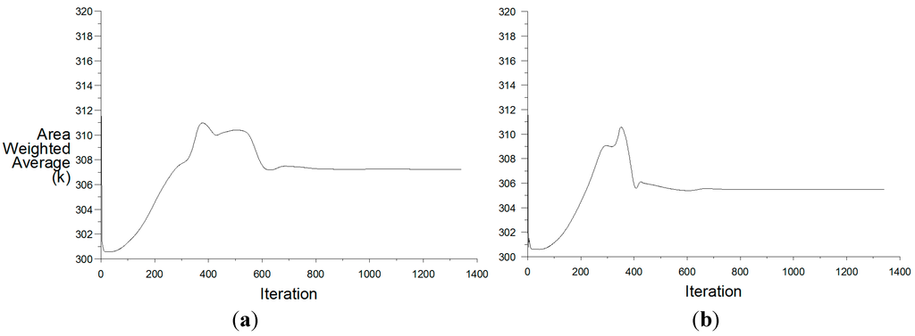
Figure 10. (a) Indoor temperature; and (b) air supply temperature convergence.

4. Experimental Methodology

The experimental test was carried out in a low speed wind tunnel detailed in [36]. The wind tunnel had a test section of the height, width, and length of 0.5 m, 0.5 m, and 1 m as shown in Figure 11. A 1:10 scale model of the wind tower and test room was used in the experimental study. According to the dimensions of the 1:10 model and the wind tunnel cross-section, the wind tower scale model produced a maximum wind tunnel blockage of 4.8%, and no corrections were made to the measurements obtained with these configurations [30,35]. Maintaining the geometric similarity between the model and prototype dimensions is necessary for accurate comparison between the two analysis methods. In order for the data measured from the scale model to be reliable, similarity is required for geometric and kinematic parameters such that the Reynolds numbers are maintained between both scales and analysis methods [37]. The geometric scale of the model of the wind tower was selected to maintain, as close as possible, equality of model and prototype ratios of overall dimensions to the important meteorological lengths of the simulated wind. All the relevant dimensions of the prototype were equally scaled down by the appropriate factor. Maintaining the ratio between the inertial and viscous forces, commonly known as the Reynolds number, for the flow has been shown to be not possible when air is used at the working fluid [38]. However, as long as the Reynolds number exceeds the critical value (10,000) for fully developed turbulent flow then the analysis is reliable [38]. The critical Reynolds number can be calculated for each scale, provided that the scale used is greater than this, fully developed turbulent flow is realised.

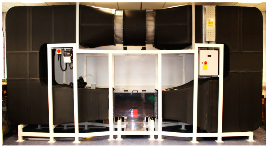
Figure 11. Closed-loop subsonic wind tunnel system for wind tower testing [36].

Due to the size of the required experimental model and complexity of the geometry, the wind tunnel prototype was created using a 3D printer. The wind tower model (Figure 12a) was connected to a 0.5 m × 0.5 m × 0.3 m room (Figure 12b), which was mounted underneath the wind tunnel test section (Figure 7). A 0.1 m × 0.1 m opening at the leeward side of the room represents the outlet. The room model was made of clear perspex sheets to allow the accurate positioning of the measurement sensors inside the room. The top plate of the room was constructed that it could be rotated in the test section in order to test different approaching wind directions.

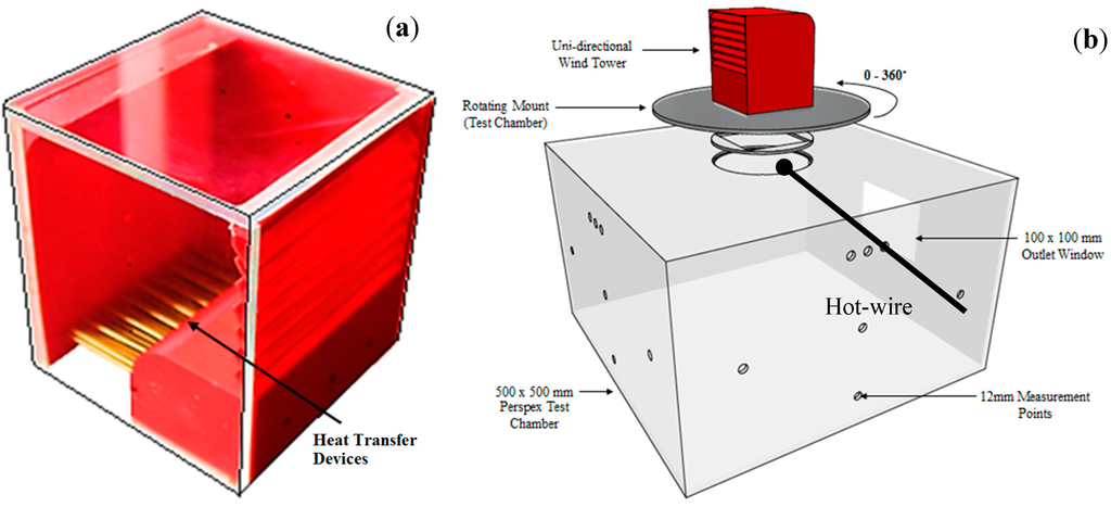
Figure 12. (a) 1:10 wind tower prototype; (b) Test room prototype.

The airflow into the room was measured using a hot-wire anemometer, which was positioned below the channels of the wind tower. The cross-sectional area of the wind tower channel was divided into several portions and the supply rate through the channel was calculated. Figure 13a shows the position of the measurement points inside the channel at a height of 0.27 m from the base of the room. The hot-wire sensor gave airflow velocity measurements with uncertainty of ±1.0% rdg. at speeds lower than 8 m/s and uncertainty of ±0.5% rdg. at higher speeds (8–20 m/s).

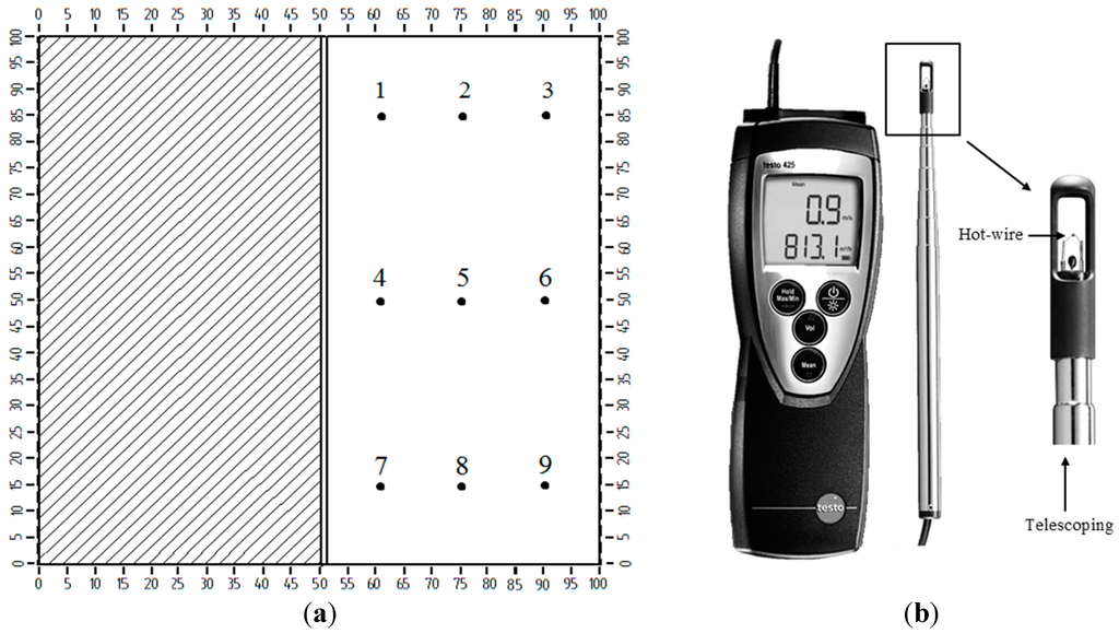
Figure 13. (a) Measurement points; (b) Hot-wire anemometer.

5. Results and Discussion

5.1. Validation of Computational Model

Figure 14a shows the comparison between the predicted and experimental results for the airflow velocity measurements below the wind tower channel. An uneven airflow distribution was observed below the supply channel. The airflow speed on the right corner of the channel (Points 1, 4 and 7) was 30%–60% higher than the left corner (Points 3, 6 and 9). This was due to the flow separation created by the sudden change in direction (90° bend). Good agreement was observed between the CFD results and measurement, with the error below 10% for all the points except for Point 6. The average error across the points was 7.2%. Figure 14b compares the CFD and experimental results of the volumetric airflow through the wind tower channel. In this figure, the direction of the airflow in the supply channel is recognised by positive and negative values of airflow. A volumetric airflow rate of 0.6 m³/s was achieved through the supply channel at 0° for an external wind speed of 3 m/s.

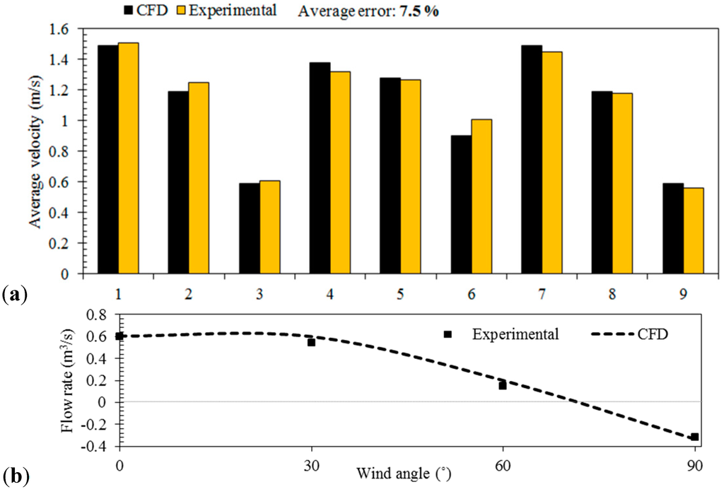
Figure 14. (a) Comparison between the prediction of the CFD and the measurement of the airflow speed at different points; (b) Effect of variation of wind direction on airflow rate.

Due to the nature of the single-sided wind tower, the dominant direction of the prevailing wind is important in obtaining maximum flow rate. At a 0° wind angle, the flow rate is at the maximum value. As the wind angle increases, the flow rate reduces to a minimum at 75°. Above this angle, negative pressure cross the opening of the wind tower causes a suction force, drawing air out shown by the negative flow rate values. Using a wind rose calculated for a specific location, the wind tower can be positioned to utilise the wind flow and direction most effectively. Should the wind the direction be 180° from the opening of the wind tower, negative pressure at the opening of the wind tower would cause air to be drawn out of the building. Though no air entering the building would pass over the heat transfer devices (HTD), ventilation would still occur as outdoor air is induced into the building through other openings.

5.2. Airflow Distribution

Figure 15a illustrates a cross-sectional plot of the velocity contours in the room and wind tower with heat transfer device. The right hand side of the plot shows the scale of airflow velocity (m/s). The contour plot in the fluid domain is colour coded and related to the CFD colour map, ranging from 0 to 3.7 m/s. As observed, the airflow passed around the wind tower, parts of it entered the wind tower and parts of it exited through the pressure outlet on the right side of the domain. After entering the wind tower, the airflow was accelerated as it hit the rear wall of the channel and re-directed downward towards the room. Separation zone was observed near the lower edge of the opening, which caused a sharp variation in velocity in this region and reduced the maximum efficiency of the wind tower. High draft speeds were observed at the centre of the room reaching up to 0.83 m/s. The air stream was circulated inside the structure and exited the opening located on the leeward side of the room. The average air velocity inside the room model was 0.28 m/s. Figure 15b shows the relation between the varying external wind speeds and performance of the wind tower in terms of the internal air distribution.

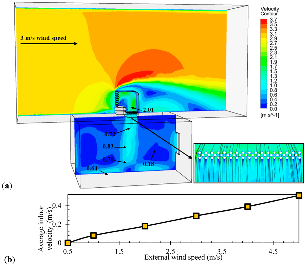
Figure 15. (a) Velocity contour plot of a cross-sectional plane; (b) Effect of variation of external wind speed on average indoor airflow speed.

5.3. Airflow Supply Rate

Since people nearly spend 90% of their time indoors, concern over human exposure to the indoor pollutants and its potential adverse effects on the occupant’s health and productivity is therefore growing. Achieving good indoor air quality in buildings, hence, depends on reducing the influence of indoor sources and also decreasing pollutant entry by effective design and operation of the ventilation system. The Building Regulation’s Approved Document F1A suggests that an air supply rate of 8–10 L/s per occupant is recommended for office spaces and classrooms [39]. A number of studies have identified that ventilation rates below 10 L/s/person affect occupants’ health and perceived air quality. In contrast, ventilation rates above 10 L/s/person are related to lower risk of Sick Building Syndrome (SBS) [40]. As shown in Table 1, the device did not meet this recommendation for an external wind speed of 1 m/s and lower. However, the system surpassed the recommended supply rates as the external velocity increased. For comparison with a standard wind tower device, the model was simulated without the heat transfer devices and the results are presented in Table 2.

Table 1. Summary of the supply rates of the wind tower with heat transfer device.

**Table 1.** Summary of the supply rates of the wind tower with heat transfer device.
Inlet Speed [m/s]	CFD Supply Rate [L/s]	CFD Supply Rate [L/s/occupant]	Building Regulation [L/s/occupant]	CFD [L/s/m²] Area = 25 m²
0.50	65.00	4.33	10.00	2.60
1.00	145.00	9.67	10.00	5.80
2.00	325.00	21.67	10.00	13.00
3.00	485.00	32.33	10.00	19.40
4.00	695.00	46.33	10.00	27.80
5.00	840.00	56.00	10.00	33.60

Table 2. Summary of the supply rates of the wind tower without heat transfer device.

**Table 2.** Summary of the supply rates of the wind tower without heat transfer device.
Inlet Speed [m/s]	CFD Supply Rate [L/s]	CFD Supply Rate [L/s/occupant]	Building Regulation [L/s/occupant]	CFD [L/s/m²] Area = 25 m²
0.50	100.00	6.67	10.00	4.00
1.00	200.00	13.33	10.00	8.00
2.00	430.00	28.67	10.00	17.20
3.00	610.00	40.67	10.00	24.40
4.00	870.00	58.00	10.00	34.80
5.00	1090.00	72.67	10.00	43.60

5.4. Temperature Distribution

Figure 16 displays a cross-sectional plot of the temperature distribution inside the room with a wind tower. The right hand side of the contour plot shows the scale of static temperature (K). The contour plot in the fluid domain is colour coded and related to the CFD colour map, ranging from 293 K (heat transfer device temperature) to 318 K (external temperature). The average temperature inside the room was 310.4 K when the temperature of the external wind was set at 318 K. The temperature was reduced further at the immediate downstream of the heat transfer device with a supply temperature value of 309 K.

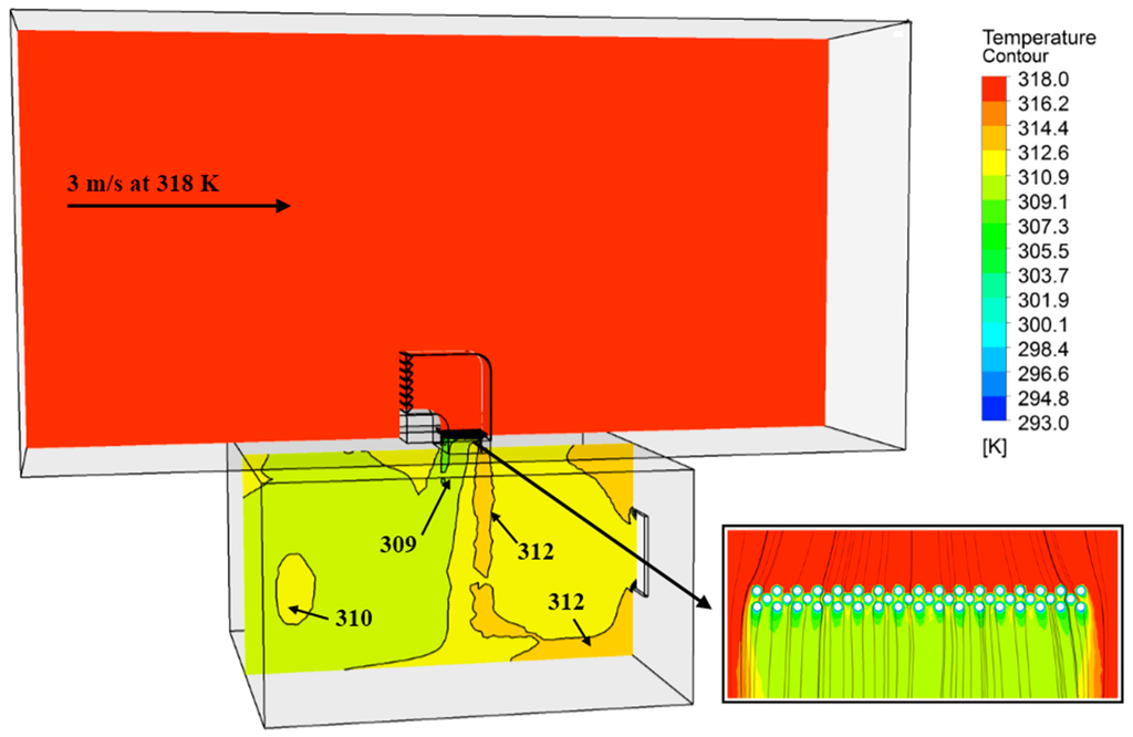
Figure 16. Cross-sectional plot of the temperature contour.

Figure 17 shows the effect of increasing the external wind speeds (1–5 m/s) on the thermal performance of the wind tower with heat transfer devices. As observed, the cooling performance of the heat transfer device decreased as the speed of the airflow increased. For instance, at 5 m/s external wind speed, the air temperature was only reduced by 5 K. Significant reduction in temperature was observed at lower wind speeds (1–2 m/s), up to 9.5–12 K reduction. Figure 18 shows the effect of varying the outdoor air temperature on the supply air temperature. The highest temperature reduction was achieved when the outdoor temperature was at 318 K and the wind speed was low (1 m/s). When the outdoor temperature was set at 302 K, the temperature reduction was only 4 K and 5 K (3 m/s and 1 m/s wind speed).

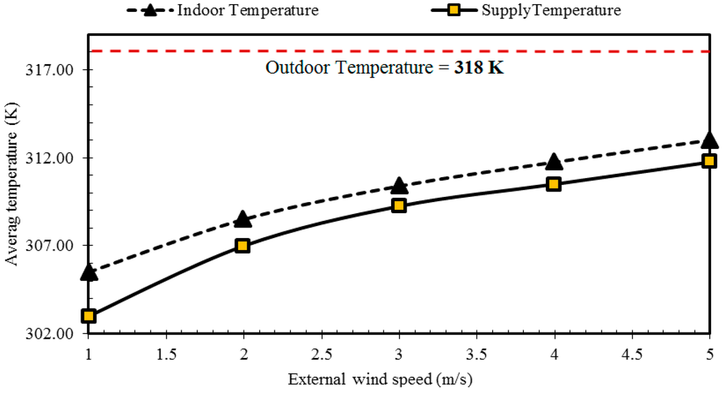
Figure 17. Effect of the wind speed on the indoor and supply air temperature.

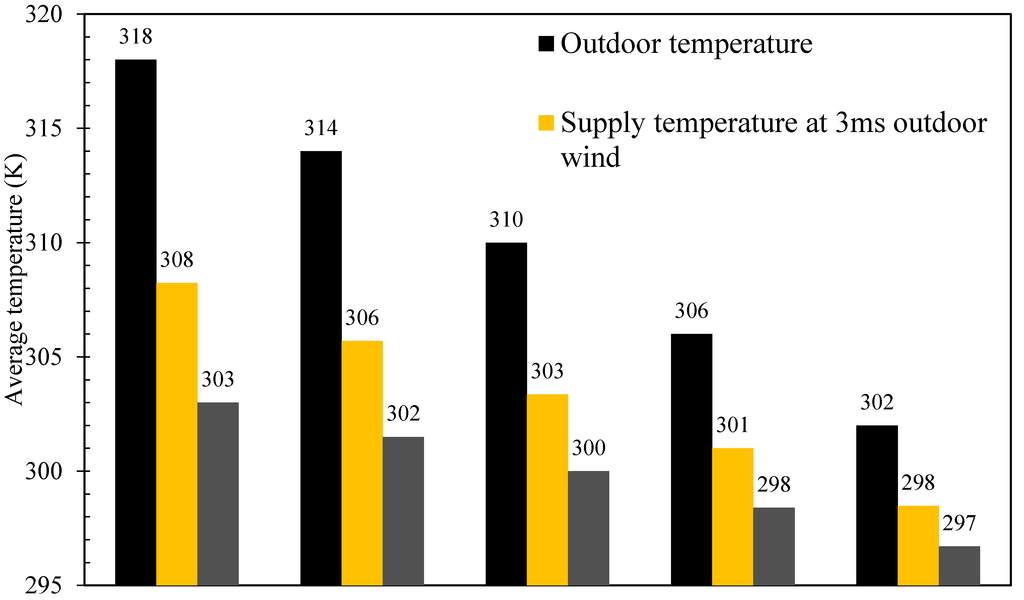
Figure 18. Effect of the outdoor temperature on the supply air temperature.

5.5. Determining the Optimum Heat Transfer Device Spacing

Figure 19 illustrates the combined response of the velocity and temperature due to the variation of the horizontal spacing between the heat transfer devices. It was observed that the effect of the horizontal spacing on the airflow temperature was more significant compared to the effect on the airflow velocity. Reducing the spacing from 100 mm to 50 mm improved the temperature drop by 3.48 K while the supply airflow velocity was reduced by only 0.12 m/s. The shaded region represents the optimum (in terms of a balance between the temperature and air velocity) horizontal spacing for the heat transfer device, and appears at 62.5–75.0 mm. U_avg and T_avg are the average predicted U and T values.

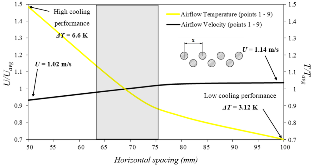
Figure 19. Effect of varying the horizontal spacing on the ventilation and thermal performance.

6. Conclusions

The integration of natural ventilation wind towers as a low energy alternative to HVAC systems has the potential to improve the thermal comfort of occupants, the indoor air quality and reduce energy consumption and greenhouse gas emissions. A comprehensive review of the advancement of Computational Fluid Dynamics (CFD) in aiding the development of wind towers was presented. From the review, it was concluded that regulating the temperature of supply air through a low energy process still remains incomplete. Therefore, a wind tower incorporating heat transfer devices was proposed to provide the link between passive ventilation and low energy temperature regulation. CFD modelling and scaled wind tunnel testing were used to evaluate the performance of the wind tower device. The CFD simulations were generally in good agreement with the experimental measurements. Simulation of different external wind speeds (1–5 m/s) showed that the cooling performance of the heat transfer device was indirectly proportional with the air supply rate. At 5 m/s external air speed, the air temperature was only reduced by 6 K. Significant reduction in the temperature was observed at lower wind speeds (1–2 m/s), up to 9.5–12 K reduction. Furthermore, the spacing between the heat transfer devices was varied to optimise the cooling and natural ventilation performance. It was found that the effect of varying the horizontal spacing on the supplied air temperature was more significant compared to the effect on the airflow velocity. Reducing the spacing from 100 mm to 50 mm improved the temperature drop by 3.48 K while the supply airflow velocity was reduced by only 0.12 m/s.

Acknowledgments

The support by the University of Sheffield (Department of Mechanical Engineering) is gratefully acknowledged. The statements made herein are solely the responsibility of the authors. The technology presented here is subject to a patent application (PCT/GB2014/052263).

Author Contributions

The main author (J.K.C.) conducted the CFD modelling and wind tunnel testing of the wind tower incorporating the heat transfer devices. The co-authors reviewed the development of CFD analysis in aiding the development of wind towers (D.O.C.) and the optimisation of natural ventilation systems (P.S.). B.R.H. participated in the analysis of the CFD and experimental data.

Conflicts of Interest

The authors declare no conflict of interest.

References

Bouchahm, Y.; Bourbia, F.; Belhamri, A. Performance analysis and improvement of the use of wind tower in hot dry climate. Renew. Energy 2011, 36, 898–906. [Google Scholar] [CrossRef]
WBCSD. Energy Efficiency in Buildings: Facts & Trends; Atar Roto Presse: Satigny, Switzerland, 2008. [Google Scholar]
Sofotasiou, P.; Hughes, B.R.; Calautit, J.K. Qatar 2022: Facing the FIFA World Cup climatic and legacy challenges. Sustain. Cities Soc. 2015, 14, 16–30. [Google Scholar] [CrossRef]
Bahadori, M.N. Passive cooling systems in Iranian architecture. Sci. Am. 1978, 238, 144–154. [Google Scholar] [CrossRef]
Hughes, B.R.; Calautit, J.K.; Ghani, S.A. The Development of Commercial Wind Towers for Natural Ventilation: A Review. Appl. Energy 2012, 92, 606–627. [Google Scholar] [CrossRef]
O’Connor, D.; Calautit, J.K.; Hughes, B.R. A Study of Passive Ventilation Integrated with Heat Recovery. Energy Build. 2014, 82, 799–811. [Google Scholar] [CrossRef]
Linden, P.F. The fluid mechanics of natural ventilation. Ann. Rev. Fluid Mech. 1999, 31, 201–238. [Google Scholar] [CrossRef]
Bahadori, M.N. An improved design of wind towers for natural ventilation and passive cooling. Sol. Energy 1985, 35, 119–129. [Google Scholar] [CrossRef]
Yaghoubi, M.A.; Sabzevari, A.; Golneshan, A.A. Wind Towers—Measurement and Performance. Sol. Energy 1991, 47, 97–106. [Google Scholar] [CrossRef]
Hughes, B.R.; Mak, C.M. A study of wind and buoyancy driven flows through commercial wind towers. Energy Build. 2011, 43, 1784–1791. [Google Scholar] [CrossRef]
Hughes, B.R.; Ghani, S.A. A numerical investigation into the effect of Windvent louvre external angle on passive stack ventilation performance. Build. Environ. 2010, 45, 1025–1036. [Google Scholar] [CrossRef]
Liu, S.C.; Mak, C.M.; Niu, J.L. Numerical Evaluation of Louver Configuration and Ventilation Strategies for the Windcatcher System. Build. Environ. 2011, 46, 1600–1616. [Google Scholar] [CrossRef]
Montazeri, H. Experimental and numerical study on natural ventilation performance of various multi-opening wind catchers. Build. Environ. 2011, 46, 370–378. [Google Scholar] [CrossRef]
Calautit, J.K.; Chaudhry, H.N.; Hughes, B.R.; Ghani, S.A. Comparison between evaporative cooling and a heat pipe assisted thermal loop for a commercial wind tower in hot and dry climatic conditions. Appl. Energy 2013, 101, 740–755. [Google Scholar] [CrossRef]
Gan, G.; Riffat, S.B. Naturally ventilated buildings with heat recovery: CFD simulation of thermal environment. Build. Serv. Eng. Res. Technol. 1997, 18, 67–75. [Google Scholar] [CrossRef]
Hughes, B.R.; Chaudhry, H.N.; Calautit, J.K. Passive energy recovery from natural ventilation air streams. Appl. Energy 2014, 113, 127–140. [Google Scholar] [CrossRef]
Calautit, J.K.; Hughes, B.R.; Chaudhry, H.N.; Ghani, S.A. CFD analysis of a heat transfer device integrated wind tower system for hot and dry climate. Appl. Energy 2013, 112, 576–591. [Google Scholar] [CrossRef]
Stavrakakis, G.; Koukou, M.; Vrachopoulos, M.; Markatos, N. Natural cross-ventilation in buildings: Building-scale experiments, numerical simulation and thermal comfort evaluation. Energy Build. 2008, 40, 1666–1681. [Google Scholar] [CrossRef]
Stavrakakis, G.; Zervas, P.; Sarimveis, H.; Markatos, N. Development of a computational tool to quantify architectural-design effects on thermal comfort in naturally ventilated rural houses. Build. Environ. 2010, 45, 65–80. [Google Scholar] [CrossRef]
Zhou, L.; Haghighat, F. Optimization of ventilation system design and operation in office environment, Part I: Methodology. Building and Environment. Build. Environ. 2009, 44, 651–656. [Google Scholar] [CrossRef]
Shen, X.; Zhang, G.; Bjerg, B. Investigation of Response Surface Methodology for Modelling Ventilation Rate of a Naturally Ventilated Building. Build. Environ. 2012, 54, 174–185. [Google Scholar] [CrossRef]
Shen, X.; Zhang, G.; Bjerg, B. Assessments of Experimental Designs in Response Surface Modelling Process: Estimating Ventilation Rate in Naturally Ventilated Livestock Buildings. Energy Build. 2013, 62, 570–580. [Google Scholar] [CrossRef]
Lal, S. Experimental, CFD simulation and parametric studies on modified solar chimney for building ventilation. Appl. Sol. Energy 2014, 50, 37–43. [Google Scholar] [CrossRef]
Calautit, J.K.; O’Connor, D.; Hughes, B.R. Determining the optimum spacing and arrangement for commercial wind towers for ventilation performance. Build. Environ. 2014, 82, 274–287. [Google Scholar] [CrossRef]
Yin, Y.; Xu, W.; Gupta, J.; Guity, A.; Marmion, P.; Manning, A.; Gulick, B.; Zhang, X.; Chen, Q. Experimental Study on Displacement and Mixing Ventilation Systems for a Patient Ward. HVAC&R Res. 2010, 15, 1175–1191. [Google Scholar] [CrossRef]
Aliabadi, A.; Faghani, E.; Tjong, H.; Green, S. Hybrid Ventilation Design for a Dining Hall Using Computational Fluid Dynamics (CFD). In Proceedings of the CSME International Congress 2014, Toronto, ON, Canada, 2014.
Chen, Q. Using computational tools to factor wind into architectural environment design. Energy Build. 2004, 36, 1197–1209. [Google Scholar] [CrossRef]
ANSYS^® Academic Research. ANSYS FLUENT User’s Guide Release 14.0. Available online: https://www.ansys.com (accessed on 1 January 2014).
Calautit, J.K.; Hughes, B.R.; Ghani, S.A. A Numerical Investigation into the Feasibility of Integrating Green Building Technologies into Row Houses in the Middle East. Archit. Sci. Rev. 2013, 56, 279–296. [Google Scholar] [CrossRef]
Calautit, J.K.; Hughes, B.R. Wind tunnel and CFD study of the natural ventilation performance of a commercial multi-directional wind tower. Build. Environ. 2014, 80, 71–83. [Google Scholar] [CrossRef]
Calautit, J.K. Integration and Application of Passive Cooling within a Wind Tower. Ph.D. Thesis, University of Leeds, Leeds, UK, 2013. [Google Scholar]
Calautit, J.K.; Hughes, B.R.; Ghani, S.A. Numerical investigation of the integration of heat transfer devices into wind towers. Chem. Eng. Trans. 2013, 34, 43–48. [Google Scholar]
Chung, T. Computational Fluid Dynamics; Cambridge University Press: Cambridge, UK, 2002. [Google Scholar]
Calautit, J.K.; Hughes, B.R. Measurement and prediction of the indoor airflow in a room ventilated with a commercial wind tower. Energy Build. 2014, 84, 367–377. [Google Scholar] [CrossRef]
Calautit, J.K.; Hughes, B.R. Integration and application of passive cooling within a wind tower for hot climates. HVAC&R Res. 2014, 20, 722–730. [Google Scholar] [CrossRef]
Calautit, J.K.; Chaudhry, H.N.; Hughes, B.R.; Sim, L.F. A validated design methodology for a closed-loop subsonic wind tunnel. J. Wind Eng. Ind. Aerodyn. 2014, 125, 180–194. [Google Scholar]
Cermak, J.E.; Isyumov, N. Wind Tunnel Studies of Buildings and Structure; ASCE Publications: Virginia, USA, 1999. [Google Scholar]
Linden, P.F.; Cooper, P. Multiple sources of buoyancy in a naturally ventilated enclosure. J. Fluid Mech. 1996, 311, 177–192. [Google Scholar] [CrossRef]
Building Regulations 2000: Approved Document F1A: Means of Ventilation. Available online: https://www.planningportal.gov.uk (accessed on 1 January 2014).
Seppänen, O.A.; Fisk, W.J.; Mendell, M.J. Association of ventilation rates and CO₂ concentrations with health and other responses in commercial and institutional buildings. Indoor Air 1999, 9, 226–252. [Google Scholar] [CrossRef] [PubMed]

© 2015 by the authors; licensee MDPI, Basel, Switzerland. This article is an open access article distributed under the terms and conditions of the Creative Commons Attribution license (http://creativecommons.org/licenses/by/4.0/).