LocRes–PINN: A Physics–Informed Neural Network with Local Awareness and Residual Learning

Abstract

Physics–Informed Neural Networks (PINNs) have demonstrated efficacy in solving both forward and inverse problems for nonlinear partial differential equations (PDEs). However, they frequently struggle to accurately capture multiscale physical features, particularly in regions exhibiting sharp local variations such as shock waves and discontinuities, and often suffer from optimization difficulties in complex loss landscapes. To address these issues, we propose LocRes–PINN, a physics–informed neural network framework that integrates local awareness mechanisms with residual learning. This framework integrates a radial basis function (RBF) encoder to enhance the perception of local variations and embeds it within a residual backbone to facilitate stable gradient propagation. Furthermore, we incorporate a residual–based adaptive refinement strategy and an adaptive weighted loss scheme to dynamically focus training on high–error regions and balance multi–objective constraints. Numerical experiments on the Extended Korteweg–de Vries, Navier–Stokes, and Burgers equations demonstrate that LocRes–PINN reduces relative prediction errors by approximately 12% to 67% compared to standard benchmarks. The results also verify the model’s robustness in parameter identification and noise resilience.

1. Introduction

Partial differential equations (PDEs) play a central role in modeling complex physical and engineering systems [1,2]. Recently, physics–informed neural networks (PINNs) have emerged as a hybrid framework that integrates data–driven learning with physical priors by embedding governing equations directly into neural network loss functions [3,4,5,6]. Raissi et al. [5] demonstrated that PINNs can achieve high accuracy and efficiency in solving both forward and inverse PDE problems, even in data–scarce regimes [7,8]. However, subsequent studies have reported that standard PINNs may suffer from optimization instability and limited capability in capturing multiscale solution features, which motivates the development of enhanced network architectures and training strategies [9,10].

Accordingly, these methodological advancements can be broadly categorized into two streams: optimization strategies and architectural innovations. Optimization–focused methods aim to enhance training dynamics via loss balancing and adaptive sampling. For example, Wang et al. [10] proposed a learning rate annealing strategy based on gradient statistics. While effective in balancing global PDE residuals and boundary constraints, it relies on global or layer–wise statistics, often overlooking local residual heterogeneity in regions with sharp physical transitions [9,10,11]. Similarly, Lu et al. [12] introduced Residual–based Adaptive Refinement (RAR) to concentrate sampling in high–error zones, and Niu et al. [11] utilized Adaptive Weighted Loss (AW–Loss) to balance multiple objectives. However, these strategies mainly operate at the data or loss level. Their effectiveness is limited by the representational capacity of the network; without an architecture capable of encoding high–frequency features efficiently, these adaptive strategies may provide diminishing returns or impose high computational costs [9,10,13,14,15].

Complementary to these optimization efforts, architectural innovations have been explored to address the inherent limitations of standard MLPs [4,6,16]. While PINNs have been applied to a wide range of PDEs, they often struggle with multiscale problems involving sharp local variations, such as boundary layers, shock waves, and discontinuities [17,18,19,20]. In such regions, the network tends to suffer from an inherent limitation in capturing high–frequency variations, leading to a noticeable decline in solution accuracy [9,10,16]. To enhance local feature representation, kernel–based methods have been introduced. For instance, Rao et al. [7] utilized general kernel functions, and Bai et al. [15] implemented radial basis function (RBF) structures. However, these approaches predominantly restrict RBFs to shallow input embeddings with minimal integration into the deep network backbone, thereby limiting the network’s global modeling capacity [21]. Conversely, increasing network depth is theoretically necessary to capture complex dynamics but often induces gradient pathologies and optimization difficulties, particularly in unsupervised learning settings [22,23,24]. To address this, researchers such as Zeng et al. [25], Tian et al. [26], and Miao et al. [27] incorporated residual connections [28] into the PINN framework to facilitate information flow and enhance convergence stability. Yet, standard residual blocks alone typically lack the specific sensitivity required to capture fine–grained local transitions in regions exhibiting abrupt physical changes. This highlights the need for a synergistic architecture that effectively integrates local feature extraction with deep residual learning.

To address the above limitations, we propose the Local–Aware Residual Physics–Informed Neural Network (LocRes–PINN), which integrates local–aware embeddings into a residual backbone to enhance accuracy and robustness. The proposed method enhances the modeling of complex physical fields without significantly increasing model complexity. In extensive numerical experiments on benchmark PDEs, LocRes–PINN consistently outperformed baseline PINNs in terms of accuracy and stability.

The main contributions of this work are summarized as follows:

(1)

We propose the RBF–Embedded Residual Network (RER–Net) to overcome the spectral bias of standard PINNs. Unlike conventional approaches that use RBFs merely as parallel distinct modules, RER–Net integrates RBF layers as embedded feature extractors within a deep residual backbone. This design enables the explicit capture of high–frequency local features while leveraging residual connections to mitigate gradient pathologies, thereby simultaneously ensuring local representational capacity and global training stability;

(2)

We incorporate a combined training strategy that leverages Residual–based Adaptive Refinement (RAR) and Adaptive Weighted Loss (AW–Loss) within our proposed architecture. This integration allows the framework to concentrate training samples in high–residual regions and dynamically balance competing loss terms. Coupled with the network’s enhanced representational capacity, these techniques improve sample efficiency and enable the model to accurately resolve steep gradients that are challenging for standard PINN architectures;

(3)

We conducted systematic experiments on representative benchmarks, including the EKdV, Navier–Stokes, and Burgers equations. Results demonstrate that LocRes–PINN consistently reduces prediction errors by 12.8% to 67% across these complex flow scenarios relative to baselines. Notably, in the inverse problem of parameter identification, the proposed method identifies physical coefficients with errors below 3%, significantly outperforming RBF–Net (which exhibits errors exceeding 17%) under identical conditions, while maintaining robustness under 20% observational noise.

2. Methodology

2.1. Overall Architecture of LocRes–PINN

We consider a general class of PDEs defined on a $d\times k-$ dimensional spatial domain Ω with boundary ∂Ω. The governing equation can be expressed as follows:

$$\begin{array}{l}N(u(\mathit{x},t))=f(\mathit{x},t),\hspace{1em}\hspace{1em}(\mathit{x},t)\in \Omega \times [{\mathrm{T}}_1,{\mathrm{T}}_2]\\ u(\mathit{x},t)=g(\mathit{x},t),\hspace{1em}\hspace{1em}(\mathit{x},t)\in \partial \Omega \times [{\mathrm{T}}_1,{\mathrm{T}}_2]\\ u(\mathit{x},0)=h(\mathit{x}),\hspace{1em}\hspace{1em}\mathit{x}\in \Omega \end{array}$$

(1)

where $N(\cdot )$ denotes the differential operator, $u(\mathit{x},t)=g(\mathit{x},t)$ represents the boundary conditions and $u(\mathit{x},0)=h(\mathit{x})$ represents the initial conditions. Let $\mathit{x}\in \Omega$ denote the spatial coordinate in a $d\times k-$ dimensional domain. Unless otherwise specified, all symbols used in the following sections are consistent with those defined here. Motivated by the need to improve local feature expressivity and global training stability, we designed LocRes–PINN to solve the defined class of PDEs. The overall architecture is illustrated in Figure 1.

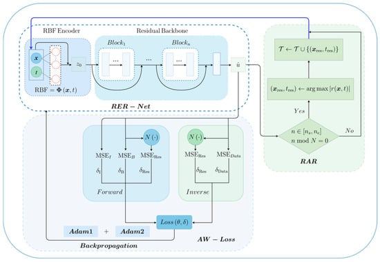
Figure 1. Schematic illustration of the Local–Aware Residual Physics–Informed Neural Network (LocRes–PINN) framework for solving partial differential equations.

The proposed LocRes–PINN framework integrates an RER–Net composed of multiple residual blocks. Given spatiotemporal input $(\mathit{x},t)$, we apply an RBF encoder to obtain localized feature representations $\mathit{\varphi }(\mathit{x},t)$. Following the encoding process, the original input is concatenated with these localized representations to form the full feature vector $z_0=[\mathit{x},t,{\mathit{\varphi }}^{x_1},{\mathit{\varphi }}^{x_2},\dots ,{\mathit{\varphi }}^{x_d},{\mathit{\varphi }}^t]$, which serves as the initial input to the network. This $z_0$ is fed into the main network, which consists of several hidden layers connected via residual connections, thereby enabling more effective modeling of multiscale features. The network outputs the predicted solution $\widehat{u}$, from which the physical residuals are computed.

To enhance the network’s representation capability in critical physical regions, we employ an iterative RAR strategy. As illustrated in the feedback loop in Figure 1, this mechanism is triggered periodically when n in [$n_s$, $n_e$] and n mod N = 0. A subset of points $({\mathit{x}}_{res},t_{res})$ corresponding to the largest residuals is selected via $\arg \max \left|r(\mathit{x},t)\right|$. These are incorporated into the training set via the update rule $\mathcal{T}\leftarrow \mathcal{T}\cup \{({\mathit{x}}_{Res},t_{Res})\}$ as part of the RAR sampling strategy, effectively updating the data pool for subsequent training iterations. The updated dataset is then used in the adaptively weighted total loss function $Loss(\theta ,\delta )$ to update loss weight parameters. To further improve training stability, a joint optimization strategy [29] is adopted, where Adam1 optimizer updates the primary network parameters $\theta$ while Adam2 optimizer adjusts the adaptive loss weights $\delta$, thereby enhancing the model’s adherence to underlying physical laws. The architectural design of RER–Net (the detailed structure of the residual block $Bloc{k}_i(i=1\dots n)$ is shown in Figure 2), the sampling strategy, and adaptive loss formulation are detailed in Section 2.2 and Section 2.3, and Section 2.4, respectively.

2.2. RER-Net

A neural network architecture is constructed to extract localized features via RBF encoding, followed by residual learning to enhance gradient stability. The design process is outlined below. The design process is outlined below. To maintain numerical stability, we adopt a unified scale compatibility criterion for all input variables prior to concatenation into $x$. Each input variable is examined and, if necessary, linearly rescaled such that its magnitude falls within the range of O (1) to O (10). This normalization principle is consistently applied to all input variables involved in the construction of $\mathit{x}$, ensuring that the inputs remain within the responsive range of the RBF kernels and avoiding gradient pathologies during the early stages of training. Variables whose natural physical scales already lie within the target range are used directly, while variables with disparate magnitudes are rescaled accordingly prior to concatenation. Concrete normalization examples for different variables are provided in the numerical experiments section. Assume an input consisting of $\mathit{x}=x_1,x_2,\dots ,x_{d-1},x_d$ and $t$, where each variable is $k-$ dimensional. Each dimension is mapped through a set of nonlinear transformations using RBF kernels. For example, the output of the $i$–th RBF unit for variable $x_1$ is defined as follows:

$$\begin{array}{l}{g}_i^{(x_1)}=-{\displaystyle \frac{{(x_1-a_i^{(x_1)}{\omega }_i^{(x_1)})}^2}{2({(b_i^{(x_1)})}^2\cdot {\sigma }_{x_1}^2+\epsilon )}},\\ {\varphi }_i^{x_1}(x_1)=e^{g_i^{(x_1)}},\hspace{1em}(i=1,\dots ,N_{x_1})\end{array}$$

(2)

where ${\varphi }_i^{x_1}(x_1)$ denotes the response of the $i$–th Gaussian RBF to variable $x_1$, and ${\omega }_i^{(x_1)}$ represents the center of the $i$–th basis function, which is fixed within the input domain $\Omega$. For a variable $x_1\in \left[x_{1,\min },x_{1,\max }\right]$, the centers are distributed as ${\omega }_i^{(x_1)}=x_{1,\min }+{\displaystyle \frac{i-1}{N_{x_1}-1}}(x_{1,\max }-x_{1,\min })$. The variance ${\sigma }_{x_1}^2$ is estimated based on the span of the input region. To control the center position, we define $a_i^{(x_1)}=1+0.5\tanh (a_{i,raw}^{(x_1)})$; the width is similarly modulated by $b_i^{(x_1)}=0.1+softplus(b_{i,raw}^{(x_1)})$. The terms $a_i^{(x_1)}$ and $b_i^{(x_1)}$ are learnable weights. A small positive constant $\epsilon$ (set to 1 × 10⁻⁸) is added to the denominator to avoid division by zero. The scalar outputs ${\varphi }_1^{x_1}(x_1),{\varphi }_2^{x_1}(x_1),\dots ,{\varphi }_{N_{x_1}}^{x_1}(x_1)$ are concatenated to form a feature vector,

$${\mathit{\varphi }}^{x_1}=({\varphi }_1^{x_1}(x_1),{\varphi }_2^{x_1}(x_1),\dots ,{\varphi }_{N_{x_1}}^{x_1}(x_1)),\hspace{1em}\hspace{1em}\hspace{1em}i=1,\dots ,N_{x_1}.$$

(3)

Following the same procedure, the RBF encodings of all input variables are obtained (with the RBF parameters adapted to the specific domain boundaries of each variable, while the number of basis functions is uniformly set to $N_{x_i}=40$ for all spatial and temporal coordinates) as ${\mathit{\varphi }}^{x_1},{\mathit{\varphi }}^{x_2},\dots ,{\mathit{\varphi }}^{x_d},{\mathit{\varphi }}^t$, which are concatenated into a unified feature vector,

$$\mathit{\varphi }(\mathit{x},t)=[{\mathit{\varphi }}^{x_1},{\mathit{\varphi }}^{x_2},\dots ,{\mathit{\varphi }}^{x_d},{\mathit{\varphi }}^t].$$

(4)

Next, the original input is concatenated with its corresponding RBF encodings to form the full input,

$$z_0=[\mathit{x},t,{\mathit{\varphi }}^{x_1},{\mathit{\varphi }}^{x_2},\dots ,{\mathit{\varphi }}^{x_d},{\mathit{\varphi }}^t].$$

(5)

A nonlinear transformation is subsequently applied, yielding

$$h_0=\tanh (W_{input}{z}_0+b_{input}).$$

(6)

where the $\tanh$ function is chosen to ensure smooth higher–order derivatives for the subsequent physics–informed loss evaluation.

$L$ residual blocks are employed, each structured as shown in Figure 2. The formulation of the $l$–th residual block is given by

$$F_l(h_l)=h_l+Linea{r}_2(\tanh (Linea{r}_1(h_l))),h_{l+1}=h_l+F_l(h_l),\hspace{1em}(l=0,\dots ,L-1)$$

(7)

Figure 2. Residual Block.

Figure 2. Residual Block.

Intuitively, this residual structure enables the network to learn the solution through incremental corrections, which significantly eases the optimization landscape compared to plain feedforward networks. Unlike standard ResNet designed for classification, this architecture omits normalization layers to maintain the integrity of the physical field values and utilizes a specific additive structure that stabilizes the backpropagation of the PDE residuals.

Finally, the output of the last residual block $h_L$ is mapped to the prediction,

$$\widehat{u}(\mathit{x},t)=W_{out}{h}_L+b_{out}$$

(8)

2.3. Initial Sampling Configuration and Loss Function Formulation

PINNs solve PDEs by embedding physical constraints directly into the loss function, enabling the learning of multidimensional solutions $\widehat{u}(\mathit{x},t)$ [4]. In this framework, neural networks are trained not only on initial and boundary conditions but also on selected observation points ${\left\{{\mathit{x}}_I^i,t_I^i,h_I^i\right\}}_{i=1}^{N_I}$ and ${\left\{{\mathit{x}}_B^i,t_B^i,g_B^i\right\}}_{i=1}^{N_B}$. To satisfy the governing equations, the model is further constrained using physical residual points ${\left\{{\mathit{x}}_{Res}^i,t_{Res}^i,f_{Res}^i\right\}}_{i=1}^{N_{Res}}$, sampled from the interior of the domain $\Omega$. In the initialization phase, these residual points are randomly sampled from a uniform distribution across the computational domain to ensure global coverage. Accordingly, we define the training loss by minimizing the mean squared error over all these sets,

$$Los{s}_{fwd}=MS{E}_I+MS{E}_B+MS{E}_{Res}$$

(9)

where

$$\begin{array}{l}MS{E}_I={\displaystyle \frac{1}{N_I}}{\displaystyle \sum _{i=1}^{N_I}{‖\widehat{u}({\mathit{x}}_I^i,0)-h_I^i‖}_2^2}\\ MS{E}_B={\displaystyle \frac{1}{N_B}}{\displaystyle \sum _{i=1}^{N_B}{‖\widehat{u}({\mathit{x}}_B^i,t_B^i)-g_B^i‖}_2^2}\\ MS{E}_{Res}={\displaystyle \frac{1}{N_{Res}}}{\displaystyle \sum _{i=1}^{N_{Res}}{‖N(\widehat{u}({\mathit{x}}_{Res}^i,t_{Res}^i))-f_{Res}^i‖}_2^2}\end{array}$$

(10)

To address inverse problems, we further introduce unknown parameters or functions $\mathit{\lambda }$, such as diffusion coefficients, source terms, or boundary condition coefficients. In this case, the governing PDEs can be reformulated in a parameterized form as follows:

$$N(u(\mathit{x},t);\mathit{\lambda })=0,\hspace{1em}\hspace{1em}\hspace{1em}(x,t)\in \Omega \times [{\mathrm{{\rm T}}}_1,{\mathrm{T}}_2]$$

(11)

Given a set of partial observations ${\{{\mathit{x}}_D^i,t_D^i\}}_{i=1}^{N_D}$, the solution must satisfy the governing equation as well as the boundary and initial conditions. On this basis, the unknown parameter $\mathit{\lambda }$ is treated as a deterministic variable rather than a stochastic quantity. The predicted solution $\widehat{u}(\mathit{x},t)$ can be jointly inferred. Consequently, the total loss for inverse problems is defined as follows:

$$Los{s}_{inv}=MS{E}_{Res}+MS{E}_{Data}$$

(12)

where $MS{E}_{Res}$ is defined in Equation (10), and the data mismatch loss $MS{E}_{Data}$ quantifies the discrepancy between the prediction and the observations. Specifically, the observational dataset ${\{{\mathit{x}}_D^i,t_D^i\}}_{i=1}^{N_D}$ is obtained by randomly sampling points from the entire spatio–temporal domain $\Omega \times [{\mathrm{T}}_1,{\mathrm{T}}_2]$. The explicit formulation is given by:

$$MS{E}_{Data}={\displaystyle \frac{1}{N_D}}{\displaystyle \sum _{i=1}^{N_D}{‖\widehat{u}({\mathit{x}}_D^i,t_D^i)-u_D^i‖}_2^2}$$

(13)

2.4. Optimization Strategy

To more effectively balance the contributions of different loss components, we adopt a dynamic adaptive weighting mechanism inspired by Niu et al. [11]. This approach leverages the Adam2 optimizer to dynamically update the relative weights of each loss term (e.g., physical residuals, and initial and boundary conditions). The updates are driven by variations in gradient magnitudes or residuals, enabling the model to adaptively adjust its learning priorities, which enhances training stability and accelerates convergence [12]. Accordingly, the loss function in Equation (9) is reformulated as follows:

$$\begin{array}{l}Loss(\theta ,\delta )={\displaystyle \frac{1}{2({\delta }_I^2+{\gamma }^{-1})}}MS{E}_I+{\displaystyle \frac{1}{2({\delta }_B^2+{\gamma }^{-1})}}MS{E}_B+{\displaystyle \frac{1}{2({\delta }_{Res}^2+{\gamma }^{-1})}}MS{E}_{Res}\\ \hspace{1em}\hspace{1em}\hspace{1em}+\log ({\delta }_I^2+{\gamma }^{-1})+\log ({\delta }_B^2+{\gamma }^{-1})+\log ({\delta }_{Res}^2+{\gamma }^{-1})\end{array}$$

(14)

where ${\delta }_I,{\delta }_B,{\delta }_{Res}$ are trainable adaptive weights corresponding to the initial condition, boundary condition, and residual losses, respectively. And these adaptive weights are updated by Adam 2 optimizer. The constant $\gamma$ is introduced to avoid numerical instability. The reformulated loss function in Equation (14) is grounded in the principle of maximum likelihood. Here, each ${\delta }_I,{\delta }_B,{\delta }_{Res}$ acts as a learnable parameter representing the homoscedastic uncertainty of its respective task. The inverse–square terms adjust the relative contribution of each loss component to balance the gradient flow, while the logarithmic terms serve as a regularization mechanism to prevent the adaptive weights from diverging to infinity during optimization. Beyond these probabilistic interpretations, adaptive weighting and sampling dynamics are further supported by control–theoretic frameworks, in particular the feedback maximum principle, which provide a mathematical foundation for optimizing supervised learning in continuity equations [30].

To enhance the network’s representation capability in critical physical regions, we employ an iterative RAR strategy [12,31]. The specific workflow is illustrated in Figure 1. Let n denote the current training iterations and $\mathcal{T}$ represent the training collocation set.

To ensure training stability and computational efficiency, the refinement process is constrained to a specific training phase n in [$n_s$, $n_e$], where $n_s$ defines the end of the warm–up period and the start of the refinement phase, and $n_e$ defines the termination iteration for the refinement. Within this range, the mechanism is triggered periodically with an interval of N iterations (i.e., when n mod N = 0).

At each trigger step, we identify the top–m candidate points {$({\mathit{x}}_{Res},t_{Res})$} corresponding to the maximum PDE residuals within the domain: $({\mathit{x}}_{Res},t_{Res})\leftarrow \arg \max \left|r(\mathit{x},t)\right|$. These identified high–error points are then dynamically appended to the current training set $\mathcal{T}$ via the update rule: $\mathcal{T}\leftarrow \mathcal{T}\cup \{({\mathit{x}}_{Res},t_{Res})\}$. This cumulative strategy allows the model to progressively focus its resources on regions with sharp gradients or complex dynamics.

The proposed LocRes–PINN framework integrates RER–Net, AW–loss, and RAR to jointly enhance model robustness and accuracy under multiscale physical dynamics and data uncertainties. The implementation details are provided in Algorithm 1.

Algorithm 1: LocRes–PINN algorithm

Input: Observed data $\{\mathit{x},t,u\}$, Collocation point counts $N_I,N_B,N_{\mathrm{Re}s},N_D$, Training configuration: error tolerance $\gamma$, RAR parameters: $n_s$, $n_e$, N, m Output: Optimized model parameters ${\theta }_{*}$, adaptive loss weights ${\delta }_{*}$, and updated residual points set $\mathcal{T}$ Construct RER–Net with:   RBF encoders $\mathit{\varphi }(\mathit{x},t)=[{\mathit{\varphi }}^{x_1},{\mathit{\varphi }}^{x_2},\dots ,{\mathit{\varphi }}^{x_d},{\mathit{\varphi }}^t]$   Concatenate $[\mathit{x},t,{\mathit{\varphi }}^{x_1},{\mathit{\varphi }}^{x_2},\dots ,{\mathit{\varphi }}^{x_d},{\mathit{\varphi }}^t]$   Input layer: Linear → SiLU   Residual Block × M (each with Linear + Tanh + Skip)   Output layer: Linear →$u_{pred}$ Initialize network parameters $\theta$ and learning rate $\eta$ Initialize adaptive weights ${\delta }_I,{\delta }_B,{\delta }_{Res}$ Initialize residual point set $\mathcal{T}={\left\{{\mathit{x}}_{\mathrm{Re}s}^i,t_{\mathrm{Re}s}^i,f_{\mathrm{Re}s}^i\right\}}_{i=1}^{N_{\mathrm{Re}s}}$ with $N_{\mathrm{Re}s}$ random collocation points For $n=0,1,\dots ,epoch$ do:   Compute physics–informed loss   Update $\theta$ using Adam1 optimizer   Update ${\delta }_I,{\delta }_B,{\delta }_{Res}$ using Adam2 optimizer   if n >= $n_s$ and n <= $n_e$ and n mod N == 0 then:     Estimate PDE residuals on candidate points     Select top–m high–residual points $({\mathit{x}}_{Res},t_{Res})\leftarrow \arg \max \left|r(\mathit{x},t)\right|$     Update training set $\mathcal{T}$ via $\mathcal{T}\leftarrow \mathcal{T}\cup \{({\mathit{x}}_{Res},t_{Res})\}$   end if   return $\theta ,{\delta }_I,{\delta }_B,{\delta }_{Res},\mathcal{T}$

3. Numerical Examples

A series of numerical experiments were conducted to evaluate the performance of the proposed LocRes–PINN in solving PDE problems. The model integrates RBF encoding with a residual neural architecture to enhance the representation of complex structures and multiscale features. To quantify the contribution of each architectural component, we designed multiple ablation studies based on LocRes–PINN, including: (i) a baseline PINN with fully connected layers; (ii) an RBF–Net with stacked RBF modules; and (iii) a ResNet employing only residual connections without RBF encoding. To ensure a fair comparison and isolate the impact of the architectural innovations, all comparative models were trained using the identical RAR and AW–Loss strategy as LocRes–PINN. Performance was evaluated in terms of accuracy, convergence rate, and numerical stability, with all models tested under the same configuration.

To rigorously evaluate model performance, the relative $L^2$–norm error is employed to quantify the discrepancy between the predicted solution $u_{pred}$ and the true solution $u_{\mathrm{t}rue}$ over the domain $\Omega$ with $K$ discrete sampling points, while the training stability is monitored via the layer–wise gradient norm $G_l={‖{\displaystyle \frac{\partial \mathcal{L}}{\partial W_l}}‖}_2$, where ${\displaystyle \frac{\partial \mathcal{L}}{\partial W_l}}$ represents the partial derivatives of the loss with respect to the weights of the l–th layer, both defined as:

$$\begin{array}{l}\mathrm{Relative}\mathrm{Error}={\left({\displaystyle \frac{{\displaystyle \sum _{i=1}^K{\left|u_{pred}(x_i)-u_{true}(x_i)\right|}^2}}{{\displaystyle \sum _{i=1}^K{\left|u_{true}(x_i)\right|}^2}}}\right)}^{{\displaystyle \frac{1}{2}}},\\ \hspace{1em}\hspace{1em}{G}_l={‖{\displaystyle \frac{\partial \mathcal{L}}{\partial W_l}}‖}_2=\sqrt{{\displaystyle \sum _{i,j}{(\frac{\partial \mathcal{L}}{\partial {\omega }_{i,j}^{(l)}})}^2}},l=1,\dots ,L.\end{array}$$

(15)

To further assess model performance, we report the experimental results of all considered models, focusing on the representational capacity and training efficiency of LocRes–PINN. To enable effective parameter optimization, a unified training strategy was adopted for the PINN, RBF–Net, ResNet, and LocRes–PINN architectures. The adaptive weight adjustment’s parameter $\gamma$ was set to 1 in the numerical experiments for all three equations. The Adam1 optimizer was used for network parameter training, with learning rates tailored to the three numerical experiments, while Adam2 with a fixed learning rate of 1 × 10⁻³ [12] was employed for the adaptive adjustment of the weights of different loss components, while other hyperparameters were kept at their default settings. The specific choices of network architecture parameters, training iterations, and collocation densities were empirically determined following established benchmarks in the PINN literature. Although these configurations are not theoretically optimal, they provide a robust baseline that balances approximation accuracy with computational efficiency for the targeted PDE problems. Observations of the training loss and solution metrics confirmed that this setup ensures stable convergence and adequately captures the multiscale features of the solutions. In terms of computational costs, “Wall–Clock Time (s)” records the total elapsed time from initialization to the completion of training, while “RAR Time (s)” denotes the cumulative duration consumed by the RAR sampling procedures.

All numerical experiments were conducted on a workstation equipped with an NVIDIA GeForce RTX 3090 GPU (24 GB) and 62.5 GB RAM. All implementations were based on the PyTorch framework (version 1.13.1) using Python 3.7.0 and were accelerated by CUDA 11.7 on a Linux system (kernel 5.4).

3.1. Extended Korteweg–De Vries Equation

Nonlinear internal waves commonly occur in stratified ocean environments, especially in coastal and continental shelf regions, where they are typically generated by tidal currents interacting with a complex topography. These waves exhibit strong nonlinearity and weak dispersion, rendering classical linear theories unable to accurately capture their propagation behavior [32]. However, from a computational perspective, the EKdV equation poses a rigorous test for PINNs. Specifically, the existence of the third–order dispersive term ${\beta }_1{u}_{xxx}$ typically leads to gradient pathology during backpropagation, while the dual nonlinearity (${\alpha }_{1}u{u}_x$ and ${\alpha }_2{u}^2{u}_x$) requires the network to capture high–frequency features and steep wave gradients without falling into local minima. As a result, the extended Korteweg–de Vries (EKdV) equation has been widely adopted as a representative model for studying such phenomena. Its general form is given by [33,34]:

$$u_t+c_0{u}_x+{\alpha }_{1}u{u}_x+{\alpha }_2{u}^2{u}_x+{\beta }_1{u}_{xxx},(x,t)\in [x_1,x_2]\times [{\mathrm{T}}_1,{\mathrm{T}}_2]$$

(16)

$$u(x,t)={\displaystyle \frac{u_0}{b+(1-b){\cosh }^2\zeta (x-ct)}},$$

(17)

where $c=c_0+{\displaystyle \frac{u_0}{3}}({\alpha }_1+{\displaystyle \frac{1}{2}}{\alpha }_2{u}_0),{\zeta }^2={\displaystyle \frac{u_0({\alpha }_1+\frac{1}{2}{\alpha }_2{u}_0)}{12{\beta }_1}},b={\displaystyle \frac{-u_0{\alpha }_2}{2{\alpha }_1+{\alpha }_2{u}_0}},$ and $u(x,t)$ is the wave amplitude. The initial condition is given by $u(x,0)={\displaystyle \frac{u_0}{b+(1-b){\cosh }^2\zeta (x)}},$ the boundary condition is $u(50,t)={\displaystyle \frac{u_0}{b+(1-b){\cosh }^2\zeta (50-ct)}},u(-50,t)={\displaystyle \frac{u_0}{b+(1-b){\cosh }^2\zeta (-50-ct)}}$ the constants are set as $c_0=0.04,{\alpha }_1=1,{\alpha }_2=-1,{\beta }_1=1,b=2/3,u_0=0.8,\zeta =0.2,x_1=-50,$ $x_2=50,$ and $[{\mathrm{T}}_1,{\mathrm{T}}_2]=[0,1].$ The primary objective of this reconstruction is to verify the model’s precision in capturing the solitary wave’s physical identity. Specifically, the accuracy is assessed by its ability to restore the peak amplitude $u_0$ and the propagation phase $c$ without significant numerical dissipation. These metrics are crucial because any slight misalignment in phase or decay in amplitude would indicate a failure of the model to satisfy the underlying conservation laws and the delicate balance between nonlinear and dispersive effects.

Because there is no publicly available dataset for this equation, high–fidelity synthetic data were generated from its analytical solution and used as the ground–truth for supervised training. In terms of network architecture, both the proposed LocRes–PINN and the ResNet models were configured with 3 residual blocks and a hidden layer width of 128. For comparison, the standard PINN consisted of 7 layers with 30 neurons per layer, and RBF–Net was set up with 9 layers. All models were trained under the same conditions: a total of 30,000 iterations using the Adam1 optimizer, an initial learning rate of 1 × 10⁻⁴, and 1000 interior PDE collocation points. Additionally, 100 initial points and 100 boundary points were used to construct the dataset. An additional 500 high–residual points were selected using the RAR strategy to improve the approximation accuracy in regions with large residuals.

In the numerical investigation of the EKdV equation, LocRes–PINN demonstrated superior modeling capability. As shown in Table 1, the mean relative errors on the test set for PINN, ResNet, RBF–Net, and LocRes–PINN were 1.144 × 10⁻³, 7.557 × 10⁻⁴, 1.503 × 10⁻³, and 4.842 × 10⁻⁴, respectively. To ensure statistical reliability, all models were evaluated across five independent trials with different random seeds, and the reported values represent the averaged performance. LocRes–PINN corresponds to an accuracy improvement of approximately 57% to 67% relative to these baseline methods. The improved accuracy is further illustrated in Figure 3, where LocRes–PINN captures steep gradient variations in the solitary–wave structure more effectively, while the baseline models exhibit a noticeable loss of accuracy in these regions. In terms of computational cost, LocRes–PINN enhances modeling performance without introducing a prohibitive overhead. The mean wall–clock time is 1348.08 s, which is lower than that of RBF–Net at 1548.0 s and only slightly higher than that of the standard PINN at 1220.87 s. In addition, the cumulative RAR time of 0.682 s indicates that the adaptive refinement strategy contributes only a negligible portion (less than 0.06%) of the total training cost.

Table 1. The mean relative Error u, Wall–Clock Time (s) and RAR Time (s) of PINN, RBF–Net, ResNet, and LocRes–PINN.

Model	PINN	RBF–Net	ResNet	LocRes–PINN
Relative Error u	1.144 × 10−3 ± 3.360 × 10−4	7.557 × 10−4 ± 3.119 × 10−4	1.503 × 10−3 ± 9.396 × 10−4	4.842 × 10−4 ± 1.545 × 10−4
Wall–Clock Time (s)	1220.87 ± 77.03	1548.0 ± 103.84	1277.70 ± 75.93	1348.08 ± 49.11
RAR Time (s)	0.496 ± 0.018	0.748 ± 0.024	0.532 ± 0.031	0.682 ± 0.052

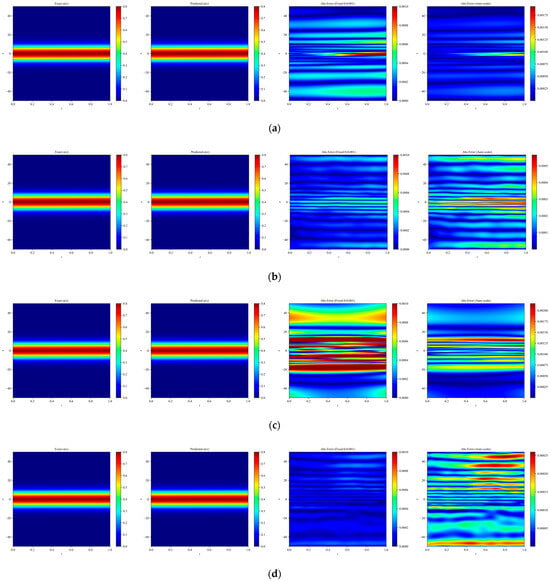
Figure 3. Heatmaps of exact and predicted solutions, along with absolute errors displayed using both fixed and independent color scales for different network architectures: (a) PINN, (b) RBF–Net, (c) ResNet, and (d) LocRes–PINN. The four columns, from left to right, correspond to the exact solution, the predicted solution, the absolute error with a fixed color scale, and the absolute error with an independent color scale. The maximum absolute errors for each model are: (a) PINN ≈ 1.75 × 10⁻³, (b) RBF–Net ≈ 5 × 10⁻⁴, (c) ResNet ≈ 2.0 × 10⁻³, and (d) LocRes–PINN ≈ 2.5 × 10⁻⁴. These heatmaps are representative examples, with performance consistent with the statistical averages.

The internal training dynamics, as analyzed via the $L_2$ gradient norms across layers in Figure 4, provide a deeper explanation for these performance disparities. While ResNet maintains a high gradient magnitude, it exhibits a sharp spike in the final layer that may lead to numerical instability; conversely, the PINN suffers from a severe “U–shaped” gradient collapse in its intermediate layers, which typically hinders the effective propagation of physical constraints. Although RBF–Net shows a steady increase in gradient norms, its upward trend suggests potential scaling challenges in deeper architectures. In contrast, LocRes–PINN demonstrates the most robust performance, utilizing local residual structures to effectively mitigate the gradient decay seen in the standard PINN and achieving a remarkably uniform gradient distribution across all layers, ensuring more balanced learning and superior numerical stability. Since all models were trained under a unified optimization strategy and computational framework, the observed performance gains can be attributed to the integrated use of RBF encoding and residual connections rather than to implementation–related differences.

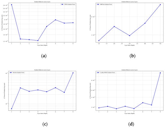
Figure 4. Gradient behavior for the Ekdv equation across different models: (a) PINN, (b) RBF–Net, (c) ResNet, and (d) LocRes–PINN.

As shown in Figure 5, LocRes–PINN achieves a high precision reconstruction of the EKdV equation. To further investigate the mechanism behind the high precision predictions observed in the snapshots, we visualize the spatiotemporal distribution of the adaptive collocation points in Figure 6. As shown, the added residual points, marked in red, are not uniformly distributed but are predominantly concentrated around the moving wavefront, where the solution exhibits steep gradients and rapid temporal variations. This observation suggests that the LocRes–PINN is able to identify regions associated with larger local residuals, which correspond to more complex physical dynamics, and to allocate additional training resources to these regions. Such an adaptive sampling behavior contributes to maintaining the accuracy of the final reconstruction.

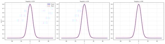
Figure 5. Results of LocRes–PINN for the Ekdv equation. The plot compares the exact solution represented by the blue solid line and the predicted solution denoted by the red dashed line at three distinct time snapshots of t = 0.2, 0.5, and 0.8. The close alignment between the curves demonstrates high prediction accuracy.

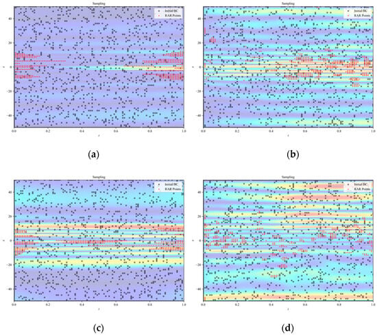
Figure 6. Sampling point distributions for the Ekdv equation across different models: (a) PINN, (b) RBF–Net, (c) ResNet, and (d) LocRes–PINN. The black dots indicate the initial collocation set consisting of 1000 randomly sampled points. The red dots represent the adaptive points added via the RAR strategy. The specific RAR configuration for this case is: start iteration $n_s=5000$, end iteration $n_e=8000$, refinement interval $N=600$, and batch size $\mathrm{m}=100$. The concentration of red dots along the wave propagation path highlights the effective capture of the steep gradients within the solitary wave structure.

To evaluate the stability and robustness of the proposed LocRes–PINN framework under realistic conditions, we investigated its performance on the Ekdv equation with varying levels of observational noise. In practical applications, measurement data are inevitably contaminated by noise; therefore, maintaining predictive accuracy under such conditions is essential. Gaussian white noise was added to the training data with intensity levels noise = {0.00, 0.01, 0.05, 0.1, 0.2}. To isolate the effect of noise intensity on convergence behavior and eliminate the influence of random initialization, all experiments were conducted using a fixed random seed. Quantitative results, including the relative error of u, wall–clock time, and RAR computation time, are reported in Table 2.

Table 2. The relative prediction error u, Wall–Clock Time (s), and RAR Time (s) of the LocRes–PINN for the Ekdv equation under various noise conditions.

Noise	0.00	0.01	0.05	0.1	0.2
Relative Error u	4.43 × 10−4	2.88 × 10−3	2.39 × 10−2	4.15 × 10−2	5.03 × 10−2
Wall–Clock Time (s)	1387.39	1422.46	1424.48	1552.40	1522.32
RAR Time (s)	0.73	0.6	0.7	0.66	0.72

As shown in Table 2, the LocRes–PINN exhibits consistent performance across different noise levels. In the noise–free case (noise = 0.00), the model achieves a relative error of 4.43 × 10⁻⁴. With increasing noise intensity, the prediction error increases gradually, as expected. Notably, even at a relatively high noise level of 20% (noise = 0.2), the relative error remains at 5.03 × 10⁻², indicating that the model retains reasonable accuracy under severe data perturbations. These results suggest that the proposed framework is capable of extracting the underlying physical dynamics from noisy observations.

In addition, the computational cost, measured by wall–clock time, remains relatively stable across all noise levels, ranging from approximately 1380 s to 1550 s. This indicates that increased noise does not significantly affect the optimization process or convergence efficiency of the LocRes–PINN. Overall, the results demonstrate that the proposed method exhibits strong robustness to observational noise, making it suitable for PDE problems where data quality cannot be fully guaranteed.

3.2. Navier–Stokes Equations in Wind Turbine Wake Flows

The Navier–Stokes (N–S) equations form the core of fluid dynamic modeling and are widely employed to simulate unsteady vortex structures and transient momentum transport within wind turbine wakes [35]. These equations are particularly effective in capturing the time–evolving nonlinear interactions and multiscale features of complex wake flows, thereby providing a robust theoretical basis for understanding dynamic wake behavior, wind–farm power prediction, and layout optimization [36]. The governing unsteady equations are

$$\begin{array}{l}{u}_t+u{u}_x+v{u}_y-{\displaystyle \frac{1}{\mathrm{Re}}}(u_{xx}+u_{yy})=0,\hspace{1em}\hspace{1em}(x,y,t)\in \Omega \times [{\mathrm{T}}_1,{\mathrm{T}}_2]\\ v_t+u{v}_x+v{v}_y-{\displaystyle \frac{1}{\mathrm{Re}}}(v_{xx}+v_{yy})=0,\\ u_x+v_y=0\end{array}$$

(18)

The Reynolds number is defined as $\mathrm{Re}=u_0\cdot D/\upsilon$, where $u,v$ are the respective stream–wise and transverse velocity components at location $(x,y)$. Following the experimental setup of Wang et al. [37], high–fidelity LiDAR measurements of wind turbine wakes were used to determine the characteristic velocity $u_0=8 \mathrm{m}/\mathrm{s}$, rotor diameter $D=126 \mathrm{m}$, and kinematic viscosity of air $\upsilon =1.5\cdot {10}^{-5} {\mathrm{m}}^2/\mathrm{s}$. The spatial domain was defined as $(x,y)\in [1374,1878]\times [1248,1752]$, and the temporal domain was $t\in [20330,20340]$. Following the data preprocessing approach outlined by Xu et al. [38], standard normalization and denormalization were applied to the equation variables and measurement data. The detailed formulations for these processes are provided in Appendix A. Assuming stationary atmospheric conditions [39], the unsteady nature of the wake flow during the observation period, we integrated the time–dependent N–S constraints with sparse wake observations to resolve the transient wake structures. This approach is particularly suitable for our objective of wind turbine wake reconstruction over the analyzed 10–s interval ($t\in [20330,20340]$). During this period, the model effectively captures the time–varying velocity deficit and the evolution of large–scale wake structures, providing a more detailed representation of the wake recovery process than traditional steady–state approximations. While this approach requires higher computational resources for unsteady–state reconstruction, it provides superior physical fidelity in capturing transient effects and mean wake dynamics simultaneously. Model performance was evaluated by comparing the velocity components $u$ and $v$, as well as the velocity magnitude $U=\sqrt{u^2+v^2}$ against the reference values through relative error analysis.

In terms of network architecture, both the proposed LocRes–PINN and the ResNet model employed 6 residual blocks with a hidden layer width of 64. The baseline PINN used 8 fully connected layers with 30 neurons per layer, while the RBF–Net was composed of 9 layers. All models were trained under identical training settings: a total of 40,000 iterations using the Adam1 optimizer, an initial learning rate of 1 × 10⁻³. The training dataset included 10,000 interior collocation points for the PDE, 1000 points for the initial condition, and 1000 points on each boundary. Additionally, 500 extra samples were introduced through the RAR strategy to iteratively enhance the solution accuracy. For model comparison, a horizontal slice of the wind turbine wake at simulation time t = 20,330 s was selected for evaluation.

In the numerical investigation of the N–S equation, LocRes–PINN demonstrated superior modeling capability. As shown in Table 3, the mean relative errors U on the test set for PINN, ResNet, RBF–Net, and LocRes–PINN were 1.693 × 10⁻², 1.038 × 10⁻², 1.068 × 10⁻², and 9.046 × 10⁻³, respectively. To ensure statistical reliability, all models were evaluated across five independent trials with different random seeds, and the reported values represent the averaged performance. LocRes–PINN corresponds to an accuracy improvement of approximately 12.8% to 46.6% relative to these baseline methods. The improved accuracy is further illustrated in Figure 7, where LocRes–PINN captures steep gradient variations in the complex wake structures more effectively, while the baseline models exhibit a noticeable loss of accuracy in these regions. The internal training dynamics, as analyzed via the $L_2$ gradient norms in Figure 8, provide a compelling explanation for the stable performance of LocRes–PINN. While the standard PINN and RBF–Net exhibit rapid gradient decay as depth increases, LocRes–PINN demonstrates a stable gradient behavior. This decay in the baseline models leads to a loss of backpropagated physical information. The pattern in LocRes–PINN confirms that the architecture acts as an essential booster. It maintains a robust gradient flow across the entire 20–layer architecture. This mechanism prevents the gradient collapse observed in baseline models and ensures that deep layers remain effectively trainable. In terms of computational cost, LocRes–PINN enhances modeling performance without introducing a prohibitive overhead. The mean wall–clock time is 4497.11 s, which is significantly lower than both RBF–Net at 13,186.01 s and ResNet at 6936.39 s, and even more efficient than the standard PINN at 5587.18 s. In addition, the cumulative RAR time of 46.46 s indicates that the adaptive refinement strategy contributes only a negligible portion (less than 1.1%) of the total training cost. As illustrated in Figure 9, this efficiency is achieved through the strategic concentration of adaptive points (red dots) within high–gradient shear layers and complex wake structures, enabling the model to capture critical flow features with minimal additional collocation points. Since all models were trained under a unified optimization strategy and computational framework, the observed performance gains can be attributed to the integrated use of RBF encoding and residual connections rather than to implementation–related differences.

Table 3. The relative prediction error u, v, U, Wall–Clock Time (s), and RAR Time (s) of PINN, RBF–Net, ResNet, and LocRes–PINN.

M.	PINN	RBF–Net	ResNet	LocRes–PINN
Relative Error u	1.692 × 10−2 ± 9.936 × 10−4	1.043 × 10−2 ± 3.683 × 10−4	1.069 × 10−2 ± 1.989 × 10−4	9.081 × 10−3 ± 5.866 × 10−5
Relative Error v	3.339 × 10−1 ± 3.246 × 10−2	2.112 × 10−1 ± 6.897 × 10−3	1.930 × 10−1 ± 1.040 × 10−2	2.294 × 10−1 ± 1.018 × 10−2
Relative Error U	1.693 × 10−2 ± 9.932 × 10−4	1.038 × 10−2 ± 3.607 × 10−4	1.068 × 10−2 ± 2.021 × 10−4	9.046 × 10−3 ± 6.756 × 10−5
Wall–Clock Time (s)	5587.18 ± 330.71	13,186.01 ± 2650.28	6936.39 ± 509.76	4497.11 ± 619.02
RAR Time (s)	22.75 ± 0.46	31.02 ± 0.73	32.38 ± 0.98	46.46 ± 3.02

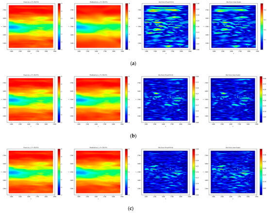
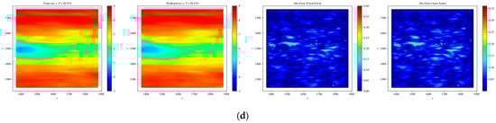
Figure 7. Heatmaps of exact and predicted solutions, along with absolute errors displayed using both fixed and independent color scales for different network architectures: (a) PINN, (b) RBF–Net, (c) ResNet, and (d) LocRes–PINN. The four columns, from left to right, correspond to the exact solution, the predicted solution, the absolute error with a fixed color scale, and the absolute error with an independent color scale. The maximum absolute errors for each model are: (a) PINN ≈ 0.4, (b) RBF–Net ≈ 0.4, (c) ResNet ≈ 0.35, and (d) LocRes–PINN ≈ 0.35. These heatmaps are representative examples, with performance consistent with the statistical averages.

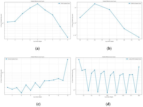
Figure 8. Gradient behavior for the N–S equation (wind turbine wake flow) across different models: (a) PINN, (b) RBF–Net, (c) ResNet, and (d) LocRes–PINN.

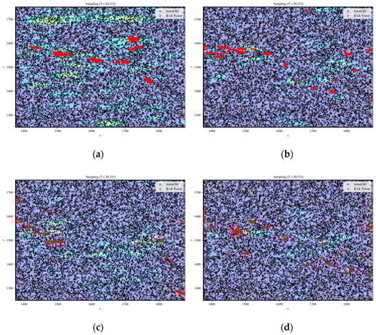
Figure 9. Sampling point distributions for the N–S equation (wind turbine wake flow) across different models: (a) PINN, (b) RBF–Net, (c) ResNet, and (d) LocRes–PINN. The black dots indicate the initial collocation set consisting of 10,000 randomly sampled points. The red dots represent the adaptive points added via the RAR strategy. The specific RAR configuration for this case is: start iteration $n_s=8000$, end iteration $n_e=\mathrm{40,000}$, refinement interval $N=8000$, and batch size $\mathrm{m}=100$. The concentration of red dots highlights the effective capture of the complex wake flow structures and high–gradient shear layers.

To evaluate the stability and robustness of the proposed LocRes–PINN framework under realistic conditions, we investigated its performance on the N–S equation with varying levels of observational noise. In practical applications, measurement data are inevitably contaminated by noise; therefore, maintaining predictive accuracy under such conditions is essential. Gaussian white noise was added to the training data with intensity levels noise = {0.00, 0.01, 0.05, 0.1, 0.2}. To isolate the effect of noise intensity on convergence behavior and eliminate the influence of random initialization, all experiments were conducted using a fixed random seed. Quantitative results, including the relative error of u, wall–clock time, and RAR computation time, are reported in Table 4.

Table 4. The relative prediction error u, v, U, Wall–Clock Time (s), and RAR Time (s) of the LocRes–PINN for the N–S equation under various noise conditions.

Noise	0.00	0.01	0.05	0.1	0.2
Relative Error u	9.16 × 10−3	9.25 × 10−3	9.57 × 10−3	1.16 × 10−2	2.38 × 10−2
Relative Error v	2.22 × 10−1	2.24 × 10−1	2.63 × 10−1	4.16 × 10−1	5.60 × 10−1
Relative Error U	9.12 × 10−3	9.21 × 10−3	9.55 × 10−3	1.15 × 10−2	2.37 × 10−2
Wall–Clock Time (s)	4615.70	4770.36	4933.98	4724.01	4943.91
RAR Time (s)	43.25	46.46	49.95	46.21	47.45

As shown in Table 4, the prediction errors of all variables increase smoothly as the noise level increases, without abrupt degradation or loss of convergence. In particular, for low to moderate noise levels. In the noise–free case (noise = 0.00), the model achieves a relative error U of 9.12 × 10⁻³. With increasing noise intensity, the prediction error increases gradually, as expected. Notably, even at a relatively high noise level of 20% (noise = 0.2), the relative error remains at 2.37 × 10⁻², indicating that the model retains reasonable accuracy under severe data perturbations. These results suggest that the proposed framework is capable of extracting the underlying physical dynamics from noisy observations.

In addition, the computational cost, measured by wall–clock time, remains relatively stable across all noise levels, ranging from approximately 4615.70 s to 4943.91 s. This indicates that increased noise does not significantly affect the optimization process or convergence efficiency of the LocRes–PINN. Overall, the results demonstrate that the proposed method exhibits strong robustness to observational noise, making it suitable for PDE problems where data quality cannot be fully guaranteed.

3.3. Inverse Problem of Burgers Equation

As a final example, the proposed LocRes–Net was employed to address the inverse problem of parameter identification in PDEs under sparse observational data. To evaluate the model’s efficacy in solving ill–posed inverse tasks, we considered the one–dimensional Burgers equation as the benchmark system. This equation is widely used as a prototypical model in fluid dynamics due to its relevance in simulating nonlinear convection-diffusion processes [8,40]. The governing equations are:

$$\begin{array}{l}{u}_t+{\lambda }_{1}u{u}_x-{\lambda }_2{u}_{xx}=0,\hspace{1em}\hspace{1em}\hspace{1em}x\in [-1,1],T\in [0,1]\\ u(x,0)=-\sin (\pi x),\\ u(t,-1)=u(t,1)=0\end{array}$$

(19)

The specific initial condition $u(x,0)=-\sin (\pi x)$ is selected because its evolution leads to the formation of a sharp shock–like discontinuity at x = 0, providing a rigorous test for the model’s ability to handle steep gradients. In this inverse problem, the parameters ${\lambda }_1$ and ${\lambda }_2$ are unknown. The training data was generated using the exact solution of the Burgers equation with the ground truth parameters set to ${\lambda }_1=1$ and ${\lambda }_2=0.01/\pi$. Because the choice of parameters ${\lambda }_1=1$ and ${\lambda }_2=0.01/\pi$ ensures a convection–dominated regime, consistent with established benchmark problems in the literature, allowing for a direct assessment of the model’s performance in parameter identification tasks. The objective of the network is to identify these two parameters from the sparse observational data.

For the network architecture, the proposed LocRes–PINN was compared against a ResNet baseline, both configured with 3 residual blocks and a hidden layer width of 64. The standard PINN used 8 layers with 30 neurons per layer, while RBF–Net was constructed with 9 layers. Training was conducted using the dataset provided by Raissi et al. [4], and the network was trained for 50,000 iterations using the Adam1 optimizer with an initial learning rate of 1 × 10⁻³. The training set consisted of 2000 randomly sampled collocation points and 300 residual points selected via the RAR strategy.

In the numerical investigation of the Burgers equation, the proposed LocRes–PINN demonstrates improved modeling performance compared to the baseline methods. As reported in Table 5, the mean relative errors of the solution u on the test set for PINN, RBF-Net, ResNet, and LocRes–PINN are 1.957 × 10⁻², 9.537 × 10⁻³, 1.589 × 10⁻², and 8.142 × 10⁻³, respectively. To ensure statistical reliability, all models were evaluated over five independent trials with different random seeds, and the reported results correspond to the averaged performance. Compared with the baseline methods, LocRes–PINN achieves a relative accuracy improvement ranging from approximately 14.6% to 58.4%. The improvement in predictive accuracy is further illustrated in Figure 10. As shown, LocRes–PINN captures the steep gradient variations of the solitary–wave structure more accurately.

Table 5. The relative prediction error u, % Error in ${\lambda }_1$, % Error in ${\lambda }_2$, Wall–Clock Time (s), and RAR Time (s) PINN, RBF–Net, ResNet, and LocRes–PINN.

Model	PINN	RBF–Net	ResNet	LocRes–PINN
Relative Error u	1.957 × 10−2 ± 5.940 × 10−3	9.537 × 10−3 ± 1.395 × 10−3	1.589 × 10−2 ± 2.833 × 10−3	8.142 × 10−3 ± 4.140 × 10−4
% Error in ${\lambda }_1$	4.114 ± 1.461	1.910 ± 0.366	4.754 ± 1.076	2.727 ± 0.563
% Error in ${\lambda }_2$	8.098 ± 4.005	17.519 ± 2.348	12.527 ± 5.053	2.412 ± 2.210
Wall–Clock Time (s)	1516.84 ± 355.66	2188.14 ± 122.25	1824.59 ± 69.54	1913.50 ± 68.22
RAR Time (s)	0.468 ± 0.076	0.806 ± 0.052	0.554 ± 0.040	0.662 ± 0.034

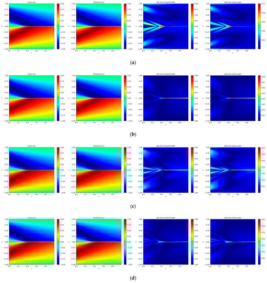
Figure 10. Heatmaps of exact and predicted solutions, along with absolute errors displayed using both fixed and independent color scales for different network architectures: (a) PINN, (b) RBF–Net, (c) ResNet, and (d) LocRes–PINN. The four columns, from left to right, correspond to the exact solution, the predicted solution, the absolute error with a fixed color scale, and the absolute error with an independent color scale. The maximum absolute errors for each model are: (a) PINN ≈ 0.08, (b) RBF-Net ≈ 0.08, (c) ResNet ≈ 0.07, and (d) LocRes-PINN ≈ 0.07. These heatmaps are representative examples, with performance consistent with the statistical averages.

Beyond field prediction, LocRes–PINN also demonstrates enhanced performance in parameter identification. Although RBF–Net attains a prediction accuracy 9.537 × 10⁻³ comparable to that of LocRes–PINN, its error in identifying the physical parameter ${\lambda }_2$ is considerably higher at 17.519%. To quantitatively investigate this discrepancy, we analyze the gradient behavior across the network layers. As shown in Figure 11, the RBF–Net architecture exhibits a pronounced ‘U–shaped’ gradient distribution where the gradient norms $G_l$ drop significantly in the intermediate layers. This localized gradient decay suggests a weakening of the backpropagation signal, which hinders the synchronized optimization of network weights and the physical parameters ${\lambda }_1$, ${\lambda }_2$. In contrast, LocRes–PINN maintains a stable gradient flow, with $G_l$ consistently staying within a healthy range of 1 × 10⁻³. This consistent gradient propagation ensures that sensitive information regarding the governing equation’s parameters is effectively preserved, leading to the lowest identification errors for both parameters, with ${\lambda }_1$ and ${\lambda }_2$ errors of 2.727% and 2.412%, respectively, as reported in Table 5. These results indicate that the integrated architecture of LocRes–PINN not only improves solution accuracy but also facilitates more accurate recovery of the underlying physical parameters in the governing equation.

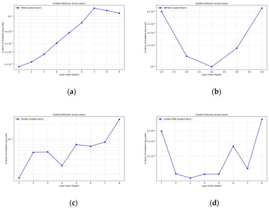
Figure 11. Gradient behavior for the Burgers equation across different models: (a) PINN, (b) RBF–Net, (c) ResNet, and (d) LocRes–PINN.

As shown in Figure 12, LocRes–PINN achieves a high–precision reconstruction of the Burgers equation. To further investigate the mechanism behind these results, we visualize the spatiotemporal distribution of the adaptive collocation points in Figure 13. As shown, the added residual points, marked in red, are predominantly concentrated along the central horizontal shock line where x = 0. This observation suggests that LocRes–PINN identifies regions with larger local residuals—corresponding to complex physical dynamics—and accordingly allocates additional training resources to these areas.

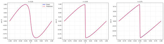
Figure 12. Results of LocRes–PINN for the Burgers equation. The plot compares the exact solution represented by the blue solid line and the predicted solution denoted by the red dashed line at three distinct time snapshots of t = 0.25, 0.5, and 0.75. The close alignment between the curves demonstrates high prediction accuracy.

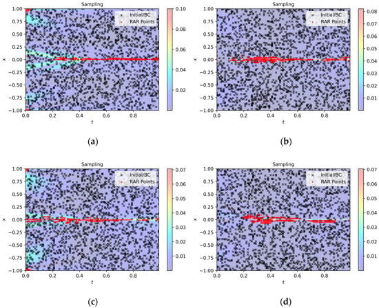
Figure 13. Sampling point distributions for the Burgers equation across different models: (a) PINN, (b) RBF–Net, (c) ResNet, and (d) LocRes–PINN. The black dots indicate the initial collocation set consisting of 2000 randomly sampled points. The red dots represent the adaptive points added via the RAR strategy. The specific RAR configuration for this case is: start iteration $n_s=\mathrm{20,000}$, end iteration $n_e=\mathrm{30,000}$, refinement interval $N=2500$, and batch size $\mathrm{m}=100$. The concentration of red dots near x = 0 highlights the effective capture of the shock wave discontinuity.

The strategic concentration of sampling points observed in Figure 10 directly facilitates the model’s ability to extract underlying physical laws from imperfect data. As a quantitative validation, Table 6 summarizes the identification results for the Burgers equation parameters under various noise levels. It can be observed that across all tested noise conditions (ranging from 0 to 0.2), the proposed method correctly identifies the leading–order structure of the equation. The identified convection coefficient ${\lambda }_1$ and diffusion coefficient ${\lambda }_2$ consistently maintain the same order of magnitude as their true physical values. While the overall parameter identification error shows limited growth as the noise level increases, the relative error for ${\lambda }_1$ remains strictly within 5%, and the error for ${\lambda }_2$ stays below 7% even at the highest noise intensity. It is worth noting that the diffusion coefficient exhibits higher sensitivity to noise, which is consistent with the characteristic of high–order derivatives being prone to noise amplification during numerical computation. These results demonstrate that the proposed method can stably perform parameter identification even under moderate noise levels, reflecting its significant robustness when dealing with noisy data.

Table 6. Identified Burgers equation coefficients ${\lambda }_1$ and ${\lambda }_2$ under different noise conditions compared with the true values $u_t+u{u}_x-0.0031831u_{xx}=0$.

Noise	Identified PDE	Error of ${\mathit{\lambda }}_{\mathbf{1}}$	Error of ${\mathit{\lambda }}_{\mathbf{2}}$
0.00	$u_t+0.97247u{u}_x-0.00316u_{xx}=0$	2.75%	0.84%
0.01	$u_t+0.96925u{u}_x-0.00314u_{xx}=0$	3.08%	1.23%
0.05	$u_t+0.95491u{u}_x-0.00332u_{xx}=0$	4.51%	4.17%
0.1	$u_t+0.97850u{u}_x-0.00337u_{xx}=0$	2.15%	5.85%
0.2	$u_t+0.96404u{u}_x-0.00298u_{xx}=0$	3.60%	6.45%

4. Conclusions and Future Work

We proposed LocRes–PINN, a physics–informed neural network framework that integrates RBF encoding and residual connections to enhance local feature representation and global training stability when solving nonlinear partial differential equations. With the integration of RBF encoding, residual skip connections, RAR sampling, and dynamic loss weighting, the proposed model achieved superior numerical performance on benchmark problems, including the EKDV equation, wind turbine wake reconstruction, and parameter identification for the Burgers equation.

Extensive numerical experiments on the EKdV equation, wind turbine wake flows, and the Burgers equation demonstrate that LocRes–PINN achieves a superior balance between accuracy and computational efficiency compared to standard PINNs and their variants. Specifically, LocRes–PINN achieved relative errors of 4.842 × 10⁻⁴ for the EKdV equation, 9.046 × 10⁻³ for the N–S equation, and 8.142 × 10⁻³ for the Burgers equation, representing accuracy improvements ranging from approximately 12.8% to 67% over baseline methods. In terms of computational cost, the model proved highly efficient; for instance, in the N–S equation case, its wall–clock time of 4497.11 s was significantly lower than that of RBF–Net and ResNet, while the RAR sampling procedure across all cases consumed a negligible portion of the total training time, typically less than 1.1%. Ablation studies further indicate that while the core RER–Net architecture provides the primary representational capacity, the RAR strategy offers auxiliary refinement for specific high–gradient features; detailed comparative results are provided in Appendix B.2. Furthermore, LocRes–PINN exhibited robust performance under observational noise levels up to 20%, maintaining reasonable relative errors (e.g., 5.03 × 10⁻² for EKdV and 2.37 × 10⁻² for N-S) and stable parameter identification for the Burgers equation, where errors for ${\lambda }_1$ and ${\lambda }_2$ remained within 3.60% and 6.45% respectively. Furthermore, while our results exhibit strong empirical consistency, there remains an open and promising research path to more formally characterize the theoretical synergy between the adaptive loss weighting and the sampling mechanisms to further strengthen the mathematical foundations of the convergence process.

Beyond these theoretical considerations, several specific avenues are identified to further enhance the practical performance and broaden the general applicability of LocRes–PINN: (1) Future research will address the theoretical gap in convergence analysis by investigating the formal approximation properties and error bounds of the RBF–embedded residual architecture, particularly for nonlinear PDEs with high–frequency features or sharp gradients. (2) We aim to investigate the interaction dynamics between the adaptive weighted loss and the RAR strategy. This includes exploring principled criteria for synchronizing loss weighting with point refinement to enhance convergence consistency across disparate physical scales. (3): The framework’s scalability will be extended to more complex physical systems, such as 3D turbulent flows and multiphysics coupling problems, to evaluate the robustness of local feature perception in higher–dimensional computational domains. (4) Efforts will be made to develop adaptive mechanisms for determining RBF kernel centers and sampling thresholds, aiming to reduce reliance on manual configuration and improve model adaptability under sparse or uncertain observations.

Appendix B.1. Training and Collocation Parameters

We summarize the key hyperparameters used in training, including the configurations for Adam1 and Adam2 optimizers, training iterations, batch sizes, collocation points, boundary points, and RAR update intervals. The number of collocation points was chosen based on literature benchmarks and practical experience. While no formal convergence study with respect to collocation density was conducted, preliminary observations indicate stable convergence and sufficient resolution for the considered PDE problems. Table A1 provides a complete overview of these settings.

Table A1. Detailed hyperparameter configurations and spatiotemporal sampling strategies for different PDE equations.

Equation	Adam1	Adam2	Iterations	I	B	Res	RAR	${\mathit{n}}_{\mathit{s}}$	${\mathit{n}}_{\mathit{e}}$	$\mathit{N}$
Ekdv	1 × 10−4	1 × 10−3	30,000	100	100	1000	500	5000	8000	600
N-S	1 × 10−3	1 × 10−3	40,000	1000	1000	10,000	500	8000	40,000	8000
Burgers	1 × 10−3	1 × 10−3	50,000	2000			300	20,000	30,000	2500

Table A1. Detailed hyperparameter configurations and spatiotemporal sampling strategies for different PDE equations.

Equation	Adam1	Adam2	Iterations	I	B	Res	RAR	${\mathit{n}}_{\mathit{s}}$	${\mathit{n}}_{\mathit{e}}$	$\mathit{N}$
Ekdv	1 × 10−4	1 × 10−3	30,000	100	100	1000	500	5000	8000	600
N-S	1 × 10−3	1 × 10−3	40,000	1000	1000	10,000	500	8000	40,000	8000
Burgers	1 × 10−3	1 × 10−3	50,000	2000			300	20,000	30,000	2500

The parameters I, B, and Res denote the number of collocation points for initial conditions, boundary conditions, and the interior domain, respectively. RAR represents the total number of residual points added through the adaptive sampling strategy. For the optimization configuration, Adam 1 and Adam 2 refer to the learning rates for the primary network parameters and the adaptive loss weights, respectively. Regarding the RAR execution, $n_s$ and $n_e$ signify the starting and ending iteration of the refinement process, while $N$ specifies the refinement interval. Specifically, for the Burgers inverse problem, 2000 collocation points are directly and randomly sampled within the spatiotemporal domain to facilitate parameter identification. All other hyperparameters follow the default settings unless otherwise specified.

Appendix B.2. Ablation Study of the RAR Strategy on Prediction Accuracy

To evaluate the specific contribution of the RAR strategy, a comparative study was performed between the complete LocRes–PINN framework and a modified version in which the RAR module was removed. Throughout the comparison, the experimental setup was strictly controlled to ensure fairness. In particular, the total number of residual collocation points was kept the same for both models, and all remaining hyperparameters, including the network architecture, learning rates, and optimization configurations, were held constant. The results presented in Table A2 indicate that the inclusion of the RAR strategy generally leads to lower prediction errors across the benchmark equations and yields smaller standard deviations.

Table A2. Impact of RAR on model performance across EKdV, N–S, and inverse Burgers equation.

Model	Ekdv	N-S	Burgers	Burgers (% Error in ${\mathit{\lambda }}_{\mathbf{1}}$)	Burgers (% Error in ${\mathit{\lambda }}_{\mathbf{2}}$)
LocRes-PINN (Without RAR)	6.341 × 10−4 ± 2.329 × 10−4	9.148 × 10−3 ± 6.213 × 10−5	8.379 × 10−3 ± 5.78 × 10−4	2.8134 ± 0.622	2.393 ± 2.132
LocRes-PINN (With RAR)	4.842 × 10−4 ± 1.545 × 10−4	9.046 × 10−3 ± 6.756 × 10−5	8.142 × 10−3 ± 4.140 × 10−4	2.727 ± 0.563	2.412 ± 2.210

Table A2. Impact of RAR on model performance across EKdV, N–S, and inverse Burgers equation.

Model	Ekdv	N-S	Burgers	Burgers (% Error in ${\mathit{\lambda }}_{\mathbf{1}}$)	Burgers (% Error in ${\mathit{\lambda }}_{\mathbf{2}}$)
LocRes-PINN (Without RAR)	6.341 × 10−4 ± 2.329 × 10−4	9.148 × 10−3 ± 6.213 × 10−5	8.379 × 10−3 ± 5.78 × 10−4	2.8134 ± 0.622	2.393 ± 2.132
LocRes-PINN (With RAR)	4.842 × 10−4 ± 1.545 × 10−4	9.046 × 10−3 ± 6.756 × 10−5	8.142 × 10−3 ± 4.140 × 10−4	2.727 ± 0.563	2.412 ± 2.210

References

- Jiao, L.; Song, X.; You, C.; Liu, X.; Li, L.; Chen, P.; Tang, X.; Feng, Z.; Liu, F.; Guo, Y.; et al. AI meets physics: A comprehensive survey. Artif. Intell. Rev. 2024, 57, 256. [Google Scholar] [CrossRef]
- Cai, S.; Mao, Z.; Wang, Z.; Yin, M.; Karniadakis, G.E. Physics-informed neural networks (PINNs) for fluid mechanics: A review. Acta Mech. Sin. 2021, 37, 1727–1738. [Google Scholar] [CrossRef]
- Raissi, M.; Yazdani, A.; Karniadakis, G.E. Hidden fluid mechanics: Learning velocity and pressure fields from flow visualizations. Science 2020, 367, 1026–1030. [Google Scholar] [CrossRef]
- Cuomo, S.; Di Cola, V.S.; Giampaolo, F.; Rozza, G.; Raissi, M.; Piccialli, F. Scientific machine learning through physics–informed neural networks: Where we are and what’s next. J. Sci. Comput. 2022, 92, 88. [Google Scholar] [CrossRef]
- Raissi, M.; Perdikaris, P.; Karniadakis, G.E. Physics-informed neural networks: A deep learning framework for solving forward and inverse problems involving nonlinear partial differential equations. J. Comput. Phys. 2019, 378, 686–707. [Google Scholar] [CrossRef]
- Karniadakis, G.E.; Kevrekidis, I.G.; Lu, L.; Perdikaris, P.; Wang, S.; Yang, L. Physics-informed machine learning. Nat. Rev. Phys. 2021, 3, 422–440. [Google Scholar] [CrossRef]
- Rao, C.; Sun, H.; Liu, Y. Physics-informed deep learning for incompressible laminar flows. Theor. Appl. Mech. Lett. 2020, 10, 207–212. [Google Scholar] [CrossRef]
- Chen, Z.; Liu, Y.; Sun, H. Physics-informed learning of governing equations from scarce data. Nat. Commun. 2021, 12, 6136. [Google Scholar] [CrossRef]
- Krishnapriyan, A.S.; Gholami, A.; Zhe, S.; Kirby, R.M.; Mahoney, M.W. Characterizing possible failure modes in physics-informed neural networks. In Proceedings of the Advances in Neural Information Processing Systems, Online, 6–14 December 2021; Curran Associates Inc.: Red Hook, NY, USA, 2021; Volume 34, pp. 26548–26560. Available online: https://proceedings.neurips.cc/paper/2021/file/df438e5206f31600e6ae4af72f2725f1-Paper.pdf (accessed on 9 January 2026).
- Wang, S.; Teng, Y.; Perdikaris, P. Understanding and mitigating gradient flow pathologies in physics-informed neural networks. SIAM J. Sci. Comput. 2021, 43, A3055–A3081. [Google Scholar] [CrossRef]
- Niu, P.; Guo, J.; Chen, Y.; Feng, M.; Shi, Y. Improved physics-informed neural network in mitigating gradient-related failures. Neurocomputing 2025, 638, 130167. [Google Scholar] [CrossRef]
- Lu, L.; Meng, X.; Mao, Z.; Karniadakis, G.E. DeepXDE: A deep learning library for solving differential equations. SIAM Rev. 2021, 63, 208–228. [Google Scholar] [CrossRef]
- Berrone, S.; Pintore, M. Meshfree Variational-Physics-Informed Neural Networks (MF-VPINN): An Adaptive Training Strategy. Algorithms 2024, 17, 415. [Google Scholar] [CrossRef]
- Zhao, C.; Zhang, F.; Lou, W.; Wang, X.; Yang, J. A comprehensive review of advances in physics-informed neural networks and their applications in complex fluid dynamics. Phys. Fluids 2024, 36, 101301. [Google Scholar] [CrossRef]
- Bai, J.; Liu, G.R.; Gupta, A.; Alzubaidi, L.; Feng, X.Q.; Gu, Y. Physics-informed radial basis network (PIRBN): A local approximating neural network for solving nonlinear partial differential equations. Comput. Methods Appl. Mech. Eng. 2023, 415, 116290. [Google Scholar] [CrossRef]
- Urbán, J.F.; Stefanou, P.; Pons, J.A. Unveiling the optimization process of Physics Informed Neural Networks: How accurate and competitive can PINNs be? J. Comput. Phys. 2025, 523, 113656. [Google Scholar] [CrossRef]
- Wight, C.L.; Zhao, J. Solving Allen–Cahn and Cahn–Hilliard equations using the adaptive physics-informed neural networks. Commun. Comput. Phys. 2021, 29, 930–954. [Google Scholar] [CrossRef]
- Moschou, S.P.; Hicks, E.; Parekh, R.Y.; Mathew, D.; Majumdar, S.; Vlahakis, N. Physics-informed neural networks for modeling astrophysical shocks. Mach. Learn. Sci. Technol. 2023, 4, 035032. [Google Scholar] [CrossRef]
- Bararnia, H.; Esmaeilpour, M. On the application of physics informed neural networks (PINN) to solve boundary layer thermal-fluid problems. Int. Commun. Heat Mass Transf. 2022, 132, 105890. [Google Scholar] [CrossRef]
- Liu, L.; Liu, S.; Xie, H.; Xiong, F.; Yu, T.; Xiao, M.; Liu, L.; Yong, H. Discontinuity computing using physics-informed neural networks. J. Sci. Comput. 2024, 98, 22. [Google Scholar] [CrossRef]
- Fu, Z.; Xu, W.; Liu, S. Physics-informed kernel function neural networks for solving partial differential equations. Neural Netw. 2024, 172, 106098. [Google Scholar] [CrossRef]
- Hughes, T.J.R.; Papadrakakis, M.; Zohdi, T. Of computer methods in applied mechanics and engineering. Comput. Methods Appl. Mech. Eng. 2022, 397, 115206. [Google Scholar] [CrossRef]
- Basir, S.; Senocak, I. Critical investigation of failure modes in physics-informed neural networks. In Proceedings of the AIAA SCITECH 2022 Forum, San Diego, CA, USA, 3–7 January 2022; AIAA: San Diego, CA, USA, 2022; p. 2353. [Google Scholar] [CrossRef]
- Mishra, S.; Molinaro, R. Estimates on the generalization error of physics-informed neural networks for approximating PDEs. IMA J. Numer. Anal. 2023, 43, 1–43. [Google Scholar] [CrossRef]
- Zeng, J.; Li, X.; Dai, H.; Zhang, L.; Wang, W.; Zhang, Z.; Kong, S.; Xu, L. A Residual Physics-Informed Neural Network Approach for Identifying Dynamic Parameters in Swing Equation-Based Power Systems. Energies 2025, 18, 2888. [Google Scholar] [CrossRef]
- Tian, R.; Kou, P.; Zhang, Y.; Mei, M.; Zhang, Z.; Liang, D. Residual-connected physics-informed neural network for anti-noise wind field reconstruction. Appl. Energy 2024, 357, 122439. [Google Scholar] [CrossRef]
- Miao, Z.; Chen, Y. VC-PINN: Variable coefficient physics-informed neural network for forward and inverse problems of PDEs with variable coefficient. Physica D 2023, 456, 133945. [Google Scholar] [CrossRef]
- He, K.; Zhang, X.; Ren, S.; Sun, J. Deep residual learning for image recognition. In Proceedings of the IEEE Conference on Computer Vision and Pattern Recognition (CVPR), San Francisco, CA, USA, 18–20 June 1996; IEEE: Las Vegas, NV, USA, 2016; pp. 770–778. [Google Scholar] [CrossRef]
- Bischof, R.; Kraus, M.A. Multi-objective loss balancing for physics-informed deep learning. Comput. Methods Appl. Mech. Eng. 2025, 439, 117914. [Google Scholar] [CrossRef]
- Staritsyn, M.; Pogodaev, N.; Chertovskih, R.; Pereira, F.L. Feedback Maximum Principle for Ensemble Control of Local Continuity Equations: An Application to Supervised Machine Learning. IEEE Control Syst. Lett. 2022, 6, 1046–1051. [Google Scholar] [CrossRef]
- Mao, Z.; Meng, X. Physics-informed neural networks with residual/gradient-based adaptive sampling methods for solving partial differential equations with sharp solutions. Appl. Math. Mech. 2023, 44, 1069–1084. [Google Scholar] [CrossRef]
- Huang, S.; Wang, J.; Li, Z.; Yang, Z.; Lu, Y. Generation characteristics of internal solitary waves in the Northern Andaman sea based on MODIS observations and numerical simulations. Front. Mar. Sci. 2024, 11, 1472554. [Google Scholar] [CrossRef]
- Helfrich, K.R.; Melville, W.K. Long nonlinear internal waves. Annu. Rev. Fluid Mech. 2006, 38, 395–425. [Google Scholar] [CrossRef]
- Flamarion, M.V.; Pelinovsky, E. Solitary wave interactions with an external periodic force: The extended Korteweg-de Vries framework. Mathematics 2022, 10, 4538. [Google Scholar] [CrossRef]
- Cai, K.; Wang, J. Physics-informed neural networks for solving incompressible Navier–Stokes equations in wind engineering. Phys. Fluids 2024, 36, 121303. [Google Scholar] [CrossRef]
- Ali, K.; Stallard, T.; Ouro, P. A diffusion-based wind turbine wake model. J. Fluid Mech. 2024, 1001, A13. [Google Scholar] [CrossRef]
- Wang, L.; Chen, M.; Luo, Z.; Zhang, B.; Xu, J.; Wang, Z.; Tan, A.C.C. Dynamic wake field reconstruction of wind turbine through physics-informed neural network and sparse LiDAR data. Energy 2024, 291, 130401. [Google Scholar] [CrossRef]
- Xu, S.; Dai, Y.; Yan, C.; Sun, Z.; Huang, R.; Guo, D.; Yang, G. On the preprocessing of physics-informed neural networks: How to better utilize data in fluid mechanics. J. Comput. Phys. 2025, 528, 113837. [Google Scholar] [CrossRef]
- Vahidi, D.; Porté-Agel, F. A physics-based model for wind turbine wake expansion in the atmospheric boundary layer. J. Fluid Mech. 2022, 943, A49. [Google Scholar] [CrossRef]
- Ortiz Ortiz, R.D.; Martínez Núñez, O.; Marín Ramírez, A.M. Solving viscous burgers’ equation: Hybrid approach combining boundary layer theory and physics-informed neural networks. Mathematics 2024, 12, 3430. [Google Scholar] [CrossRef]
Disclaimer/Publisher’s Note: The statements, opinions and data contained in all publications are solely those of the individual author(s) and contributor(s) and not of MDPI and/or the editor(s). MDPI and/or the editor(s) disclaim responsibility for any injury to people or property resulting from any ideas, methods, instructions or products referred to in the content. |
© 2026 by the authors. Licensee MDPI, Basel, Switzerland. This article is an open access article distributed under the terms and conditions of the Creative Commons Attribution (CC BY) license.