Abstract
Most solutions of fractional differential equations (FDEs) that model real-world phenomena in various fields of science, industry, and engineering are complex and cannot be solved analytically. This paper mainly aims to present some useful results for studying the qualitative properties of solutions of FDEs involving the new generalized Hattaf mixed (GHM) fractional derivative, which encompasses many types of fractional operators with both singular and non-singular kernels. In addition, this study also aims to unify and generalize existing results under a broader operator. Furthermore, the obtained results are applied to some linear systems arising from medicine.
1. Introduction
Fractional differential equations (FDEs) have become a powerful tool for modeling complex systems that exhibit nonlocal dynamics, memory effects, hereditary properties, and anomalous behavior, which cannot be accurately described using classical ordinary differential equations (ODEs). For example, FDEs have been used in biology to model biological complexity, from subcellular processes to ecosystem dynamics. Their ability to capture memory, heterogeneity, and anomalous transport makes them a significant contributor to the development of predictive biology, precision medicine, and bioengineering.
In the literature, FDEs have been widely applied across many fields, and they have been formulated by means of various fractional operators, such as the Caputo fractional derivative [1], the Caputo–Fabrizio (CF) fractional derivative [2], the Atangana–Baleanu (AB) fractional derivative [3], the weighted AB fractional derivative [4], the generalized Hattaf fractional (GHF) derivative [5], the Hattaf mixed fractional derivative [6], the Hadamard fractional derivative [7,8] and the Katugampola fractional derivative [9]. More recently, a new generalized Hattaf mixed (GHM) fractional derivative was introduced in [10] to include all the above-cited fractional derivatives [1,2,3,4,5,6,7,8,9] as well as other types, such as the new weighted fractional derivative with respect to another function [11], the generalized AB fractional derivative, the derivative involving the generalized Mittag-Leffler function [12], the AB fractional derivative with respect to another function [13], the weighted CF fractional derivative with respect to another function [14], the power fractional derivative [15], as well as the modified fractional derivative [16].
Several researchers have studied the qualitative analysis of FDEs based on various inequalities. For instance, Aguila-Camacho et al. [17] established a useful inequality for the Caputo fractional derivative of the quadratic Lyapunov function to prove the stability of numerous fractional systems. This useful inequality was extended to investigate the stability of FDEs with the AB fractional derivative [18], the Hadamard fractional derivative [19], the GHF derivative [20], as well as the generalized proportional Caputo fractional derivative [21]. Another idea proposed by Vargas-De-León [22] aimed to extend the Volterra-type Lyapunov function to fractional-order epidemic systems via an inequality, allowing one to estimate the Caputo fractional derivative of this function. Similarly, the last inequality was extended to the Caputo fractional derivative with respect to another function in [23], to the GHF derivative in [20], and to the AB fractional derivative in [18].
On the other hand, the stability analysis of fractional nonlinear systems involving the Caputo fractional derivative was studied by Delavari et al. [24] by means of Bihari and Bellman–Gronwall inequalities [25,26]. An extension of the comparison principle to the Hadamard fractional derivative was used by Wang et al. [27] to analyze the stability of a class of nonlinear Hadamard-type fractional differential systems. A new version of the fractional comparison principle was introduced in [28] to discuss the qualitative properties of FDEs with the GHF derivative, such as stability, asymptotic stability, and Mittag-Leffler stability. This new version extends the results presented in [29] for the Caputo fractional derivative and the one in [24] for the Riemann–Liouville fractional derivative.
In recent years, FDEs have received growing interest in pharmacokinetics and other medical-related applications due to their ability to capture nonlocal dynamics, long-term memory effects, and anomalous behaviors, making them a powerful tool for modeling complex biomedical systems. Their flexibility also makes FDEs particularly suitable for pharmacokinetics, biomedical signal processing, tumor growth, and disease modeling, enabling more accurate predictions, improved data fitting, and enhanced clinical decision-making. In [30], the authors investigated the application of FDEs to analyze datasets related to various drug processes exhibiting anomalous kinetics. Awadalla et al. [31] modeled drug concentration in human blood using the Psi-Caputo fractional derivative. The dynamics of a tumor growth model involving the Caputo fractional derivative were analyzed in [32]. In 2024, Wanassi and Torres [33] proposed a fractional model for blood alcohol concentration based on the same Psi-Caputo derivative, aiming to better capture the long-range dependencies and memory effects that play an important role in modeling blood alcohol concentration. The role of fractional derivatives in pharmacokinetic/pharmacodynamic anesthesia model using bispectral index scale (BIS) data was more recently investigated by Vellappandi and Lee [34].
The contributions of this study are as follows: (i) to extend the aforementioned inequalities, and (ii) to establish significant and practical results for investigating the qualitative properties of FDEs involving the GHM fractional derivative, aiming to unify and generalize a broad class of fractional operators with both singular and non-singular kernels. The choice of this fractional operator is motivated by its nonlocal nature and high flexibility. It allows for the adjustment of a wide range of parameters, making it particularly suitable for fitting real data and accurately capturing complex real-world dynamics. Moreover, the GHM fractional derivative incorporates a kernel with multiple tunable parameters, enabling it to represent various types of memory effects, including exponential, power-law, and Mittag-Leffler kernels, within a unified framework. To achieve the objectives of this study, the remainder of this paper is organized as follows: Section 2 introduces key preliminary concepts and results required for the subsequent analysis. Section 3 is devoted to the main results of the study, including generalizations of several known inequalities and the extension of the comparison principle to the GHM fractional derivative. Section 4 presents an application of our main analytical results to linear systems in the field of medicine. Finally, Section 5 concludes this paper, summarizing the main results, comparing them with related studies, highlighting their potential for extension to other applications, and outlining directions for future research.
2. Preliminary Concepts and Results
This section recalls the concepts related to the new GMH fractional derivative and presents some preliminary results necessary for the present study.
Definition 1
([10]). Assume that , , , , , , and . The GHM fractional derivative of the function of order α in the Caputo sense with the weight function and with respect to another function is defined as follows:
where is a normalization function, satisfying , with on the interval ; is the generalized Mittag-Leffler function with three parameters [35], with and denoting the Pochhammer symbol; and .
It is important to note that the GHM fractional derivative given by Definition 1 includes numerous fractional derivatives with singular and non-singular kernels available in the literature. As examples, it becomes the Caputo fractional derivative [1] when , , and ; the CF fractional derivative [2] when , , and ; the AB fractional derivative [3] when , , , and ; the weighted AB fractional derivative [4] when , , and ; the GHF derivative [5] when and ; the Hattaf mixed fractional derivative [6] when , , and ; the Hadamard fractional derivative [7,8] when , and ; the Katugampola fractional derivative [9] when , , and with ; the new weighted fractional derivative with respect to another function [11] when ; the generalized AB fractional derivative with the generalized Mittag-Leffler function [12] when , , , and ; the AB fractional derivative with respect to another function [13] when , , and ; the weighted CF fractional derivative with respect to another function [14] when ; the CF fractional derivative with respect to another function [14] when and ; the power fractional derivative [15] when , , (with ) and ; the modified fractional derivative [16] when , , , , and ; as well as the fractional derivative introduced in [36] when , , , , and .
Now, we recall the fractional integral associated with the GHM fractional derivative.
Definition 2
([10]). When , the fractional integral corresponding to the GHM fractional derivative is given by
where is the weighted Riemann–Liouville fractional integral of the the function with respect to another function [37] defined by
for and .
The generalized Hattaf fractional integral introduced in Definition 2 covers many forms of fractional integrals, including the generalized weighted fractional integral with respect to another function [11], the GHF integral [5], the fractional integral corresponding to the generalized AB fractional derivative with the generalized Mittag-Leffler function [12], the weighted AB fractional integral [4], the AB fractional integral with respect to another function [13], the AB fractional integral [3], the weighted CF fractional integral with respect to another function [14], the CF fractional derivative [2], the fractional integral corresponding to the new mixed fractional derivative [6], the power fractional integral [15], the fractional integral introduced in [36], the modified fractional integral [16], the weighted Riemann–Liouville fractional integral with respect to another function [37], the Hadamard fractional integral [38,39], the Katugampola fractional integral [40], the Riemann–Liouville fractional integral [41], the Riemann–Liouville fractional integral with respect to another function [41,42,43], and the tempered fractional integral [44,45].
Next, we recall the following fundamental result, which extends the Newton–Leibniz formula presented in [41] to the Caputo fractional derivative with a singular kernel, in [6] for the mixed fractional derivative, and in [46] to the AB fractional derivative in the Caputo sense.
Lemma 1.
Let , , , , and . Then
Based on Theorem 2.6 of [10], we deduce the following result.
Lemma 2.
The weighted Laplace transform with respect to another function χ of the GHM fractional derivative is given as follows:
where
3. Main Results
Let g be a continuous function and u be a continuously differentiable function. For any constant , we consider the following function:
Hence, we have the following:
We define
Thus,
where
Theorem 1.
For any constant , the GHM fractional derivative of the function defined by (4) satisfies the following inequalities:
- (i)
- When g is an increasing function and or , we have
- (ii)
- When g is a decreasing function and or , we have
Proof.
From integration by parts and using , with , we obtain the following:
Since , we have the following:
We define the following function:
Obviously, . When g is an increasing function, the function is decreasing on the interval and increasing on , with . Thus, has the global minimum at . Hence,
As , we obtain for all . Similarly, we can easily prove that for all when g is a decreasing function. This proves when .
For , the expression of is as follows:
Since , we have . Hence,
This proves for . □
Corollary 1.
Let be a continuously differentiable function. Then, at any time , for or , we have the following:
Proof.
By applying Theorem 1 (i) to the function , we have the following:
This completes the proof of Corollary 1. □
Remark 1.
Corollary 1 generalizes and extends various results existing in the literature. For instance,
- When , and , we get Corollary 1 of [20] for the GHF derivative.
- When , , and , we obtain Lemma 3.1 of [18] for the AB fractional derivative.
- When , and , we get Lemma 1 of [17] for the Caputo fractional derivative.
- When , and , we get Remark 3 of [19] for the Caputo fractional derivative.
- When , and with , we obtain Lemma 1 of [21] for the generalized proportional Caputo fractional derivative [47,48].
Corollary 2.
Let be a continuously differentiable function and . Then, at any time , for or , we have the following:
Proof.
For , we have .
Since is a decreasing function on , it follows from Theorem 1 (ii) that
which implies that
Then,
Since , we have the following:
This completes the proof of Corollary 2. □
Remark 2.
Corollary 2 generalizes and extends many inequalities used to establish the global stability of FDEs. For example,
- When and , we obtain the recent result presented in Theorem 5 of [23].
- When , and , we get Corollary 2 of [20] for GHF derivative.
- When , and , we get Lemma 3.1 of [22] for the Caputo fractional derivative.
- When , , and , we obtain Lemma 3.2 of [18] for the AB fractional derivative.
Theorem 2.
Let be a continuously differentiable function and be a symmetric positive definite matrix. Then, at any time , for or , we have the following:
Proof.
Consider the following function:
Then
where . Hence,
Integrating by parts, for , we obtain the following:
Since , we have the following:
On the other hand, the expression of for is as follows:
Since , we have . It follows from the Hospital’s rule that
Hence,
Therefore, for all when or , which implies that
The proof is completed. □
Remark 3.
Theorem 2 extends and generalizes many recent results reported in previous studies. More precisely, Theorem 2 coincides with
- (i)
- Lemma 2.5 of [49] when , and with ;
- (ii)
- Corollary 1 of [23] when , and ;
- (iii)
- Lemma 1 of [50] when , and , which covers the results presented in [18,20,51].
Theorem 3.
(Fractional comparison principle). Let and be two functions defined on the interval with and . Then for all .
Proof.
Since , it follows from Lemma 1 that
which leads to
As , we have , for all . □
Remark 4.
Theorem 3 extends three results, as follows: The first is in Lemma 6.1 of [29] involving the Caputo fractional derivative; the second is in Theorem 2.4 of [24] involving the Riemann–Liouville fractional derivative, and the third is in Lemma 1 of [28] involving the GHF derivative.
As in [37], the weighted convolution of functions f and g is defined by
Obviously, we have
Theorem 4.
Let κ be a constant, and be two functions such that
- (i)
- If , thenwhere and .
- (ii)
- If , then
Proof.
By applying the weighed Laplace transform to both sides of (11) and using Lemma (2), for , we obtain the following:
Since , we have
Hence,
This proves (i). For , we have
which implies that
This proves (ii). □
Corollary 3.
Let and be a function such that
- (i)
- If , then
- (ii)
- If , then
Proof.
It follows from (12) that there exists a nonnegative function such that
According to Theorem 4, for , we have the following:
Since and for , we get
Similarly, for , we obtain the following:
Hence,
□
Remark 5.
Corollary 3 includes the result given in [50]; it suffices to take and in .
Corollary 4.
Let , and be two nonnegative functions such that
- (i)
- If , then
- (ii)
- If , then
Proof.
Let . By applying Theorem 4, for , we have the following:
Since , we have
In a similar way, for , we obtain the following:
This completes the proof. □
Remark 6.
Corollary 4 covers the χ-Caputo Bellman–Gronwall inequality presented in Theorem 3 of [23]; it suffices to take in .
4. Application
This section presents an application of the main results obtained to investigate a problem in pharmacokinetics, which is a branch of medicine that studies the absorption, distribution, metabolism, and elimination of drugs in a living body.
To describe the dynamics of a drug concentration in a living body, we propose the following mathematical model with linear FDEs involving the GHM fractional derivative:
where represents the drug concentration in the body at time t, d is a positive constant that can be experimentally determined for each drug, and denotes the initial drug dose administered.
The drug concentration model presented by system (14) captures the time evolution of a drug within the body, governed by absorption, distribution, metabolism, and elimination. The GHM fractional derivative used in system (14) accounts for delayed drug absorption, heterogeneous tissue diffusion, and long-term retention, which are commonly observed in real biological systems.
By applying Theorem 4 for the case , the solution of (14) is given by
In this situation, the pharmacokinetics model presented in 2022 by Awadalla et al. [31] for predicting drug concentration levels in human blood over time is a special case of (14). Furthermore, the solution of (14) given by (15) is reduced to that presented in [31] by choosing .
For the situation , the application of Theorem 4 yields the solution of (14) as follows:
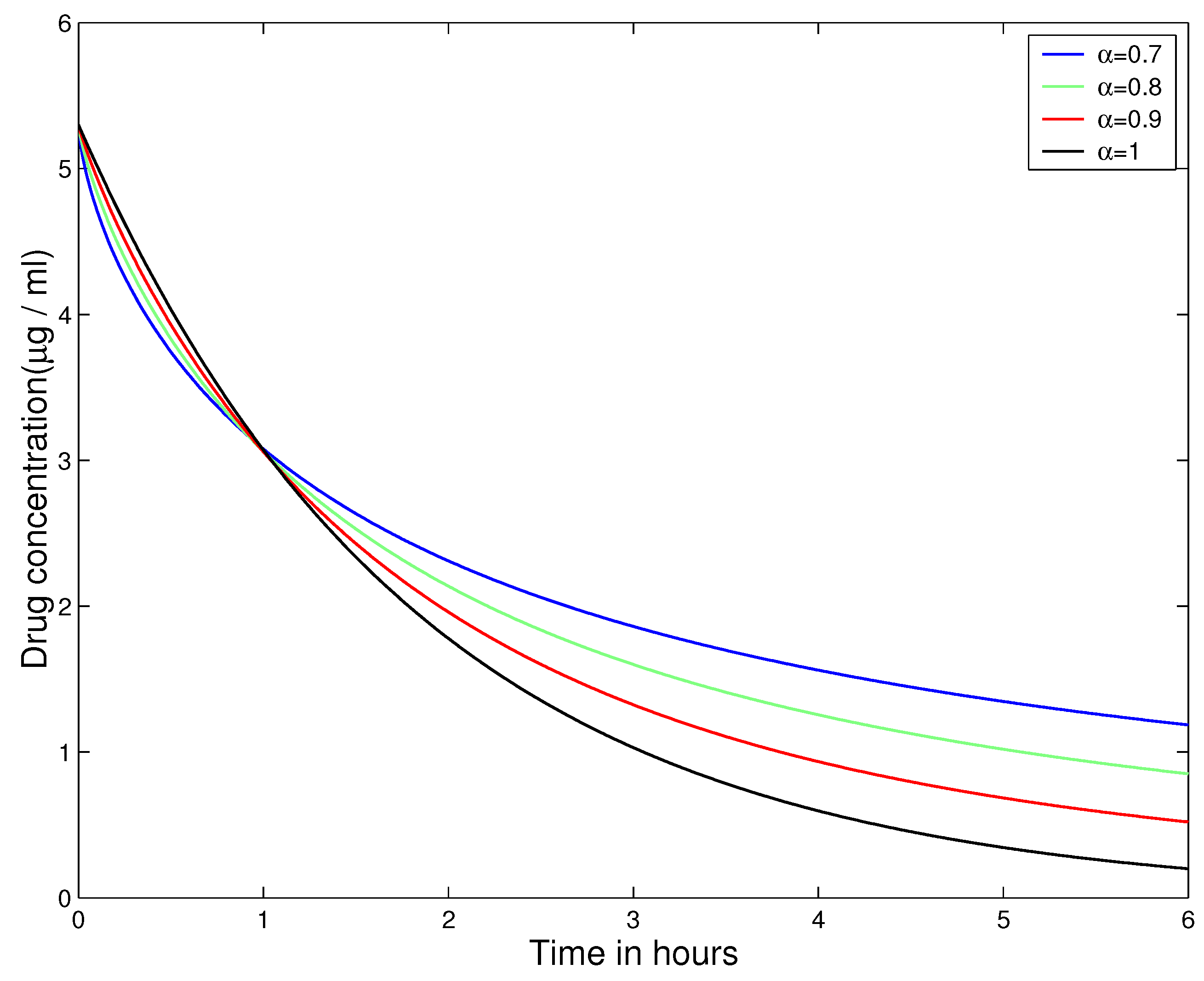
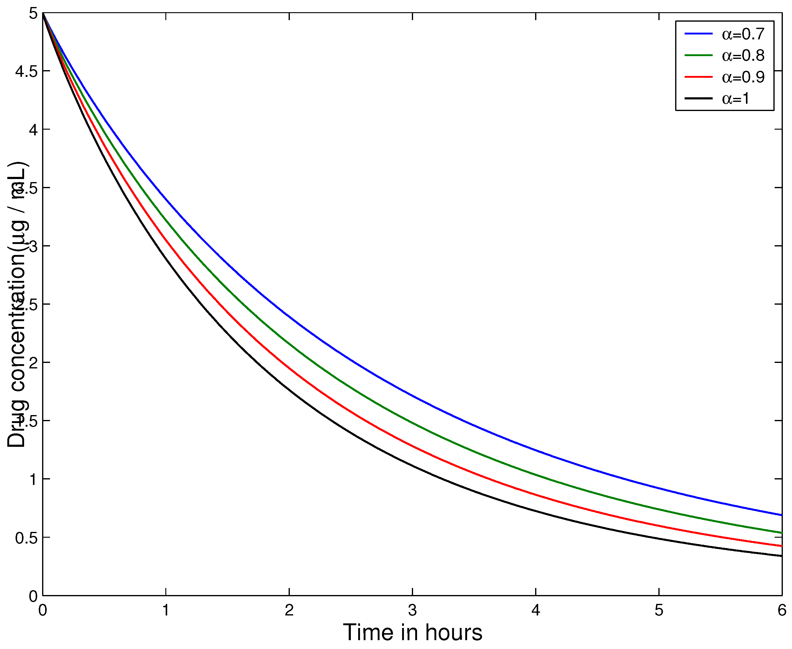
Let , , , and . Figure 1 and Figure 2 present the graphs of solutions of the pharmacokinetics model (14) for different values of order .
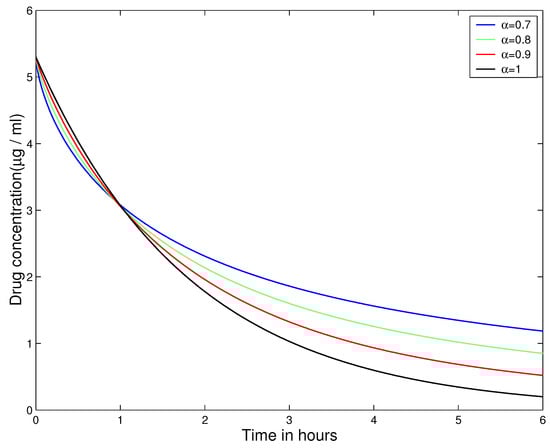
Figure 1.
The graph of (15) for different values of order .
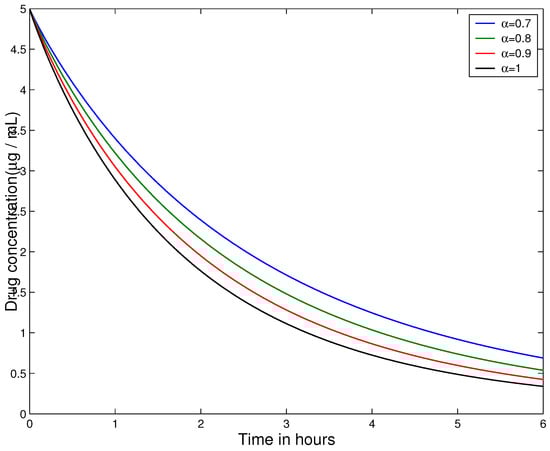
Figure 2.
The graph of (16) for different values of with and .
Based on Figure 1 and Figure 2, we observe that as the fractional order decreases, the memory effect becomes more pronounced, leading to a slower decay of drug concentration. This behavior reflects the nonlocal and history-dependent nature of fractional-order models, which more accurately capture the dynamics of real biological systems compared to classical models. Additionally, the slower decay of drug concentration at lower fractional orders may correspond to slow diffusion or delayed drug absorption due to complex bio-macromolecular interactions.
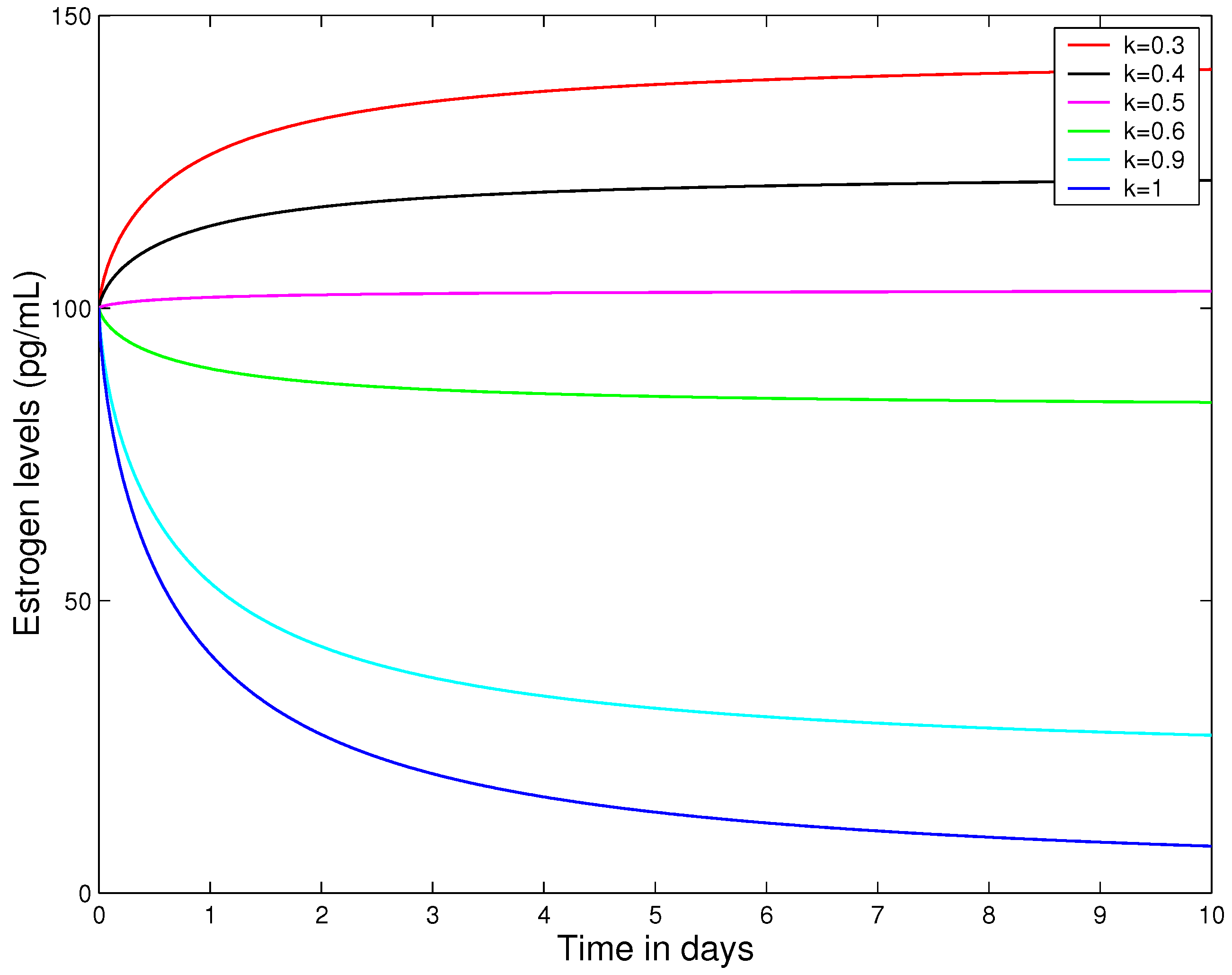
In medicine, various hormone therapies are employed to either lower estrogen levels or balance estrogen with other hormones. One such drug, Tamoxifen, is primarily used to treat hormone-dependent breast cancer by blocking estrogen receptors, which prevents cancer cells from utilizing estrogen for growth. Apart from cancer treatment, Tamoxifen is also applied in managing other conditions associated with excess estrogen. To investigate the impact of this drug on estrogen dynamics, we consider the following model:
where represents the estrogen levels at time t. The parameter s is the source rate of estrogen, while denotes the rate at which estrogen is washed out from the body system. Furthermore, the parameter k represents the drug efficacy.
It follows from Theorem 4 for the case that the solution of (17) is given by
When the weight function is constant, (18) is as follows
Similar to the first application example, let and . It is obvious that is the unique globally stable steady state of model (17), which represents the total amount of estrogen in the human body. However, normal estrogen levels vary by sex and life stage. In premenopausal women, levels fluctuate during the menstrual cycle, typically ranging from 15 to 350 pg/mL, while postmenopausal women have significantly lower levels, often below 10 pg/mL. In men, estrogen levels remain relatively stable throughout life (10–40 pg/mL) [52,53,54]. In addition, the washout rate of estrogen by the body is equal to day−1 [55]. Therefore, we obtain s between 0 and pg/mL/day. A complete list of parameters and their estimated values for model (17) is presented in Table 1.

Table 1.
Parameters and values of model (17).
Figure 3 shows that hormone therapy has a significant impact on estrogen dynamics, allowing high estrogen levels to be reduced to below 100 pg/mL when its efficacy exceeds .
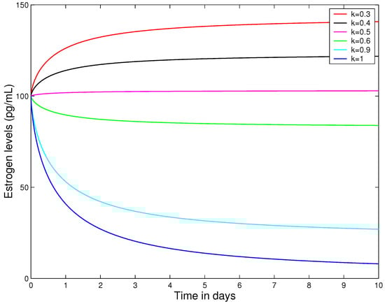
Figure 3.
The graph of (19) for different values of drug efficacy k with .
5. Conclusions
In this work, we proposed an analytical framework for studying the qualitative behavior of solutions of FDEs based on the GHM fractional derivative, which includes a broad class of fractional operators with both singular and non-singular kernels. We established a series of comparison principles and generalized Lyapunov-type inequalities that extend numerous results from previous studies. The research results were applied to some linear pharmacokinetic models in the medical field.
Based on the above results and due to the core advantages associated with the GHM fractional derivative, future research directions will focus on the stability analysis and the existence of solutions for FDEs involving the novel GHM fractional derivative, as well as the extension of application to modeling phenomena arising from ecology [56,57] and other medical fields, such as tumor growth modeling, physiological signal analysis, and infectious disease dynamics.
Funding
This research received no external funding.
Institutional Review Board Statement
Not applicable.
Informed Consent Statement
Not applicable.
Data Availability Statement
The original contributions presented in this study are included in the article. Further inquiries can be directed to the corresponding author.
Acknowledgments
The author would like to thank the editor and anonymous reviewers for their constructive comments and valuable suggestions, which significantly improved the quality of this paper.
Conflicts of Interest
The author declares no conflicts of interest.
References
- Caputo, M. Linear models of dissipation whose Q is almost frequency independent-II. Geophys. J. Int. 1967, 13, 529–539. [Google Scholar] [CrossRef]
- Caputo, M.; Fabrizio, M. A new definition of fractional derivative without singular kernel. Prog. Fract. Differ. Appl. 2015, 1, 73–85. [Google Scholar]
- Atangana, A.; Baleanu, D. New fractional derivatives with non-local and non-singular kernel: Theory and application to heat transfer model. Therm. Sci. 2016, 20, 763–769. [Google Scholar] [CrossRef]
- Al-Refai, M. On weighted Atangana-Baleanu fractional operators. Adv. Differ. Equ. 2020, 2020, 3. [Google Scholar] [CrossRef]
- Hattaf, K. A new generalized definition of fractional derivative with non-singular kernel. Computation 2020, 8, 49. [Google Scholar] [CrossRef]
- Hattaf, K. A new mixed fractional derivative with applications in computational biology. Computation 2024, 12, 7. [Google Scholar] [CrossRef]
- Gambo, Y.Y.; Jarad, F.; Baleanu, D.; Abdeljawad, T. On Caputo modification of the Hadamard fractional derivatives. Adv. Differ. Equ. 2014, 2014, 10. [Google Scholar] [CrossRef]
- Jarad, F.; Abdeljawad, T.; Baleanu, D. Caputo-type modification of the Hadamard fractional derivatives. Adv. Differ. Equ. 2012, 2012, 142. [Google Scholar] [CrossRef]
- Almeida, R.; Malinowska, A.B.; Odzijewicz, T. Fractional differential equations with dependence on the Caputo-Katugampola derivative. J. Comput. Nonlinear Dyn. 2016, 11, 061017. [Google Scholar] [CrossRef]
- Hattaf, K. A new generalized class of fractional operators with weight and respect to another function. J. Fract. Calc. Nonlinear Syst. 2024, 5, 53–68. [Google Scholar] [CrossRef]
- Thabet, S.T.M.; Abdeljawad, T.; Kedim, I.; Ayari, M.I. A new weighted fractional operator with respect to another function via a new modified generalized Mittag-Leffler law. Bound. Value Probl. 2023, 2023, 100. [Google Scholar] [CrossRef]
- Abdeljawad, T.; Baleanu, D. On fractional derivatives with generalized Mittag-Leffler kernels. Adv. Differ. Equ. 2018, 2018, 468. [Google Scholar] [CrossRef]
- Fernandez, A.; Baleanu, D. Differintegration with respect to functions in fractional models involving Mittag-Leffler functions. SSRN Electron. J. 2018, 1–5. [Google Scholar] [CrossRef]
- Al-Refai, M.; Jarrah, A. Fundamental results on weighted Caputo-Fabrizio fractional derivative. Chaos Solitons Fractals 2019, 126, 7–11. [Google Scholar] [CrossRef]
- Lotfi, E.M.; Zine, H.; Torres, D.F.M.; Yousfi, N. The power fractional calculus: First definitions and properties with applications to power fractional differential equations. Mathematics 2022, 10, 3594. [Google Scholar] [CrossRef]
- Chinchole, S.M. Modified definitions of SABC and SABR fractional derivatives and applications. Int. J. Differ. Equ. 2022, 17, 87–112. [Google Scholar]
- Aguila-Camacho, N.; Duarte-Mermoud, M.A.; Gallegos, J.A. Lyapunov functions for fractional order systems. Commun. Nonlinear Sci. Numer. Simulat. 2014, 19, 2951–2957. [Google Scholar] [CrossRef]
- Taneco-Hernández, M.A.; Vargas-De-León, C. Stability and Lyapunov functions for systems with Atangana-Baleanu Caputo derivative: An HIV/AIDS epidemic model. Chaos Solitons Fractals 2020, 132, 109586. [Google Scholar] [CrossRef]
- Dai, C.; Ma, W. Lyapunov direct method for nonlinear Hadamard-type fractional order systems. Fractal Fract. 2022, 6, 405. [Google Scholar] [CrossRef]
- Hattaf, K. On some properties of the new generalized fractional derivative with non-singular kernel. Math. Probl. Eng. 2021, 2021, 1580396. [Google Scholar] [CrossRef]
- Almeida, R.; Agarwal, R.P.; Hristova, S.; O’Regan, D. Quadratic Lyapunov functions for stability of the generalized proportional fractional differential equations with applications to neural networks. Axioms 2021, 10, 322. [Google Scholar] [CrossRef]
- Vargas-De-León, C. Volterra-type Lyapunov functions for fractional-order epidemic systems. Commun. Nonlinear Sci. Numer. Simulat. 2015, 24, 75–85. [Google Scholar] [CrossRef]
- Ma, W.; Dai, C.; Li, X.; Bao, X. On the kinetics of Ψ-fractional differential equations. Fract. Calc. Appl. Anal. 2023, 26, 2774–2804. [Google Scholar] [CrossRef]
- Delavari, H.; Baleanu, D.; Sadati, J. Stability analysis of Caputo fractional-order nonlinear systems revisited. Nonlinear Dynam. 2012, 67, 2433–2439. [Google Scholar] [CrossRef]
- Rao, M.R. Ordinary Differential Equations; East-West Press: Minneapolis, MI, USA, 1980. [Google Scholar]
- Slotine, J.J.E.; Li, W. Applied Nonlinear Control; Prentice Hall: Englewood Cliffs, NJ, USA, 1991. [Google Scholar]
- Wang, G.; Pei, K.; Chen, Y.Q. Stability analysis of nonlinear Hadamard fractional differential system. J. Frankl. Inst. 2019, 356, 6538–6546. [Google Scholar] [CrossRef]
- Hattaf, K. On the Stability and Numerical Scheme of Fractional Differential Equations with Application to Biology. Computation 2022, 10, 97. [Google Scholar] [CrossRef]
- Li, Y.; Chen, Y.Q.; Podlubny, I. Stability of fractional-order nonlinear dynamic systems: Lyapunov direct method and generalized Mittag-Leffler stability. Comput. Math. Appl. 2010, 59, 1810–1821. [Google Scholar] [CrossRef]
- Dokoumetzidis, A.; Macheras, P. Fractional kinetics in drug absorption and disposition processes. J. Pharmacokinet. Pharmacodyn. 2009, 36, 165–178. [Google Scholar] [CrossRef]
- Awadalla, M.; Noupoue, Y.Y.Y.; Asbeh, K.A.; Ghiloufi, N. Modeling drug concentration level in blood using fractional differential equation based on Psi-Caputo derivative. J. Math. 2022, 2022, 9006361. [Google Scholar] [CrossRef]
- Padder, A.; Almutairi, L.; Qureshi, S.; Soomro, A.; Afroz, A.; Hincal, E.; Tassaddiq, A. Dynamical analysis of generalized tumor model with Caputo fractional-order derivative. Fractal Fract. 2023, 7, 258. [Google Scholar] [CrossRef]
- Wanassi, O.K.; Torres, D.F.M. Modeling blood alcohol concentration using fractional differential equations based on the Ψ-Caputo derivative. Math. Methods Appl. Sci. 2024, 47, 7793–7803. [Google Scholar] [CrossRef]
- Vellappandi, M.; Lee, S. Role of fractional derivatives in pharmacokinetic/pharmacodynamic anesthesia model using BIS data. Comput. Biol. Med. 2025, 187, 109783. [Google Scholar] [CrossRef]
- Prabhakar, T.R. A singular integral equation with a generalized Mittag-Leffler function in the kernel. Yokohama Math. J. 1971, 19, 7–15. [Google Scholar]
- Chinchole, S.M.; Bhadane, A.P. A new definition of fractional derivatives with Mittag-Leffler kernel of two parameters. Commun. Math. Appl. 2022, 13, 19–26. [Google Scholar] [CrossRef]
- Jarad, F.; Abdeljawad, T.; Shah, K. On the weighted fractional operators of a function with respect to another function. Fractals 2020, 28, 2040011. [Google Scholar] [CrossRef]
- Hadamard, J. Essai sur l’étude des fonctions données par leur developpment de Taylor. J. Math. Pures Appl. Ser. 1892, 8, 101–186. [Google Scholar]
- Kilbas, A.A. Hadamard-type fractional calculus. J. Korean Math. Soc. 2001, 38, 1191–1204. [Google Scholar]
- Katugampola, U.N. New approach to a generalized fractional integral. Appl. Math. Comput. 2011, 218, 860–865. [Google Scholar] [CrossRef]
- Kilbas, A.A.; Srivastava, H.M.; Trujillo, J.J. Theory and Applications of Fractional Differential Equations; North-Holland Mathematics Studies; Elsevier: Amsterdam, The Netherlands, 2006. [Google Scholar]
- Osler, T.J. Leibniz rule for fractional derivatives generalized and an application to infinite series. SIAM J. Appl. Math. 1970, 18, 658–674. [Google Scholar] [CrossRef]
- Samko, S.G.; Kilbas, A.A.; Marichev, O.I. Fractional Integrals and Derivatives: Theory and Applications; Gordon and Breach Science: New York, NY, USA, 1993. [Google Scholar]
- Li, C.; Deng, W.; Zhao, L. Well-posedness and numerical algorithm for the tempered fractional ordinary differential equations. Discrete Contin. Dyn. Syst. Ser. B 2019, 24, 1989–2015. [Google Scholar]
- Meerschaert, M.M.; Sabzikar, F.; Chen, J. Tempered fractional calculus. J. Comput. Phys. 2015, 293, 14–28. [Google Scholar] [PubMed]
- Baleanu, D.; Fernandez, A. On some new properties of fractional derivatives with Mittag-Leffler kernel. Commun. Nonlinear Sci. Numer. Simul. 2018, 59, 444–462. [Google Scholar] [CrossRef]
- Jarad, F.; Abdeljawad, T.; Alzabut, J. Generalized fractional derivatives generated by a class of local proportional derivatives. Eur. Phys. J. Spec. Top. 2017, 226, 3457–3471. [Google Scholar] [CrossRef]
- Alzabut, J.; Abdeljawad, T.; Jarad, F.; Sudsutad, W. A Gronwall inequality via the generalized proportional fractional derivative with applications. J. Ineq. Appl. 2019, 2019, 101. [Google Scholar] [CrossRef]
- Sene, N. Stability analysis of the generalized fractional differential equations with and without exogenous inputs. J. Fract. Calc. Appl. 2019, 12, 562–572. [Google Scholar] [CrossRef]
- Hattaf, K. Stability of fractional differential equations with new generalized hattaf fractional derivative. Math. Probl. Eng. 2021, 2021, 8608447. [Google Scholar] [CrossRef]
- Sene, N. Stability analysis of the fractional differential equations with the Caputo-Fabrizio fractional derivative. J. Fract. Calc. Appl. 2020, 11, 160–172. [Google Scholar]
- Greenblatt, R.B.; Oettinger, M.; Bohler, C.S.S. Estrogen-androgen levels in aging men and women: Therapeutic considerations. J. Am. Geriatr. Soc. 1976, 24, 173–178. [Google Scholar] [CrossRef]
- Bae, Y.J.; Zeidler, R.; Baber, R.; Vogel, M.; Wirkner, K.; Loeffler, M.; Ceglarek, U.; Kiess, W.; Körner, A.; Thiery, J.; et al. Reference intervals of nine steroid hormones over the life-span analyzed by LC-MS/MS: Effect of age, gender, puberty, and oral contraceptives. J. Steroid Biochem. Mol. Biol. 2019, 193, 105409. [Google Scholar] [CrossRef]
- Petrela, R.B.; Chhetri, C.D.; Najafi, A.; Zhang, Z.; Rinkoski, T.A.; Wieben, E.D.; Fautsch, M.P.; Chakraborty, S.; Millen, A.E.; Patel, S.P. Associations between measures of oestrogen exposure and severity of Fuchs endothelial corneal dystrophy. BMJ Open Ophthalmol. 2025, 10, e001884. [Google Scholar] [CrossRef]
- Wu, C.H.; Motohashi, T.; Abdel-Rahman, H.A.; Flickinger, G.L.; Mikhail, G. Free and protein-bound plasma Estradiol-17β during the menstrual cycle. J. Clin. Endocrinol. Metab. 1976, 43, 436–445. [Google Scholar] [CrossRef] [PubMed]
- Lin, J.; Xu, C.; Xu, Y.; Zhao, Y.; Pang, Y.; Liu, Z.; Shen, J. Bifurcation and controller design in a 3D delayed predator-prey model. Aims Math. 2024, 9, 33891–33929. [Google Scholar] [CrossRef]
- Zhao, Y.; Xu, C.; Xu, Y.; Lin, J.; Pang, Y.; Liu, Z.; Shen, J. Mathematical exploration on control of bifurcation for a 3D predator-prey model with delay. Aims Math. 2024, 9, 29883–29915. [Google Scholar] [CrossRef]
Disclaimer/Publisher’s Note: The statements, opinions and data contained in all publications are solely those of the individual author(s) and contributor(s) and not of MDPI and/or the editor(s). MDPI and/or the editor(s) disclaim responsibility for any injury to people or property resulting from any ideas, methods, instructions or products referred to in the content. |
© 2025 by the author. Licensee MDPI, Basel, Switzerland. This article is an open access article distributed under the terms and conditions of the Creative Commons Attribution (CC BY) license (https://creativecommons.org/licenses/by/4.0/).