Simultaneous Multi-Objective and Topology Optimization: Effect of Mesh Refinement and Number of Iterations on Computational Cost

Abstract

In this study, a multi-objective optimization procedure with embedded topology optimization was presented. The procedure simultaneously optimizes the spatial arrangement and topology of bodies in a multi-body system. The multi-objective algorithm determines the locations of supports, joints, active loads, reactions, and load magnitudes, which serve as inputs for the topology optimization of each body. The multi-objective algorithm dynamically adjusts domain size, support locations, and load magnitudes during optimization. Due to repeated topology optimization calls within the genetic algorithm, the computational cost is significant. To address this, two reduction strategies are proposed: (I) using a coarser mesh and (II) reducing the number of iterations during the initial generations. As optimization progresses, Strategy I gradually refines the mesh, while Strategy II increases the maximum allowable iteration count. The effectiveness of both strategies is evaluated against a baseline (Reference) without reductions. By the 25th generation, all approaches achieve similar hypervolume values (Reference: 2.181; I: 2.112; II: 2.133). The computation time is substantially reduced (Reference: 42,226 s; I: 16,814 s; II: 21,674 s), demonstrating that both strategies effectively accelerate optimization without compromising solution quality.

1. Introduction

Topology optimization (TO) is a commonly used technique for designing lightweight load-bearing structures by efficiently distributing available material across a predefined domain [1]. In compliance minimization problem statements, topology optimization has been shown to improve the stiffness of a structure for a given material volume and set of input conditions within a discretized domain. The required inputs typically include domain size, support locations, available material volume fraction, and locations and magnitudes of applied loads [2]. While TO has been extended to dynamic loading scenarios [3], conventional methods generally assume fixed support locations, limiting their applicability in cases where support layouts must also be optimized.

A key limitation of traditional TO approaches is their reliance on predefined boundary conditions, which restricts their use in problems where support positions are unknown or variable. Generally, support locations are assigned on one side of the domain, leading to suboptimal solutions when real-world constraints dictate alternative layouts. To address this issue, researchers have explored methods to incorporate support location optimization within the TO framework. A comprehensive review of topology optimization methods addressing design-dependent loads and supports was conducted by [4]. Early studies provided both analytical and numerical solutions to the problem of support placement optimization [5,6,7]. Buhl [6] extended TO by treating support locations as additional design variables, adjusting their costs to guide placement selection. Similarly, Lee and Xie [7] introduced element-based support locations, which were included as additional design variables. Further, Panesar et al. [8] integrated the system and structural design aspects to enable the production of multi-functional parts with embedded components. This enabled the production of parts with optimal designs and embedded electrical components. Zhu et al. [9] further advanced this approach by optimizing component placement alongside structural configuration, facilitating the better integration of embedded elements.

However, these TO approaches primarily focus on single-domain structures and do not extend to multi-body systems, where interactions between multiple interconnected components must be considered. Multi-body topology optimization extends traditional topology optimization to systems with multiple interacting components, requiring considerations of contact mechanics, dynamic interactions, and structural constraints. Firstly, Ma et al. [10] developed a multi-domain topology optimization to enable controlled material distribution across subdomains; however, the approach was still limited to one body. Ghandriz et al. [11] optimized multiple interconnected components using the modified Solid Isotropic Material with Penalization (SIMP) method to avoid numerical instabilities, while sensitivities were approximated to reduce computational costs. However, their study did not account for variable support locations. Further, Fernandez et al. [12] aimed to solve the topology optimization problem of 3D deformable bodies in contact, which was performed using mortar segment-to-segment discretization and adjoint sensitivity analysis to improve computational efficiency. Sun and Hu [13] focused on the dynamic topology optimization of flexible multi-body systems, addressing time-varying systems and coupled optimization strategies. Fu et al. [14] integrated trajectory and topology optimization, utilizing the mode-superposition and adjoint sensitivity analysis to optimize both structure and control design variables. All the listed advancements improved the capabilities of multi-body topology optimization, making it more efficient and applicable to robotics, aerospace, and automated machinery fields. All the referenced papers solely utilize gradient-based optimization methods, which are ineffective when design variables include discrete dimensions, support locations, or actuator positions.

While gradient-based methods have been used for actuator placement and TO problems [15], they are limited to continuous design variables, struggle with discrete variables, cannot guarantee global optimality for non-convex problems [16], and are not suitable for multi-objective (MO) problems [17]. This limitation makes them less effective for problems involving multi-body systems (mechanisms in particular) where contact problems (e.g., cams, gears, or robotic grippers) introduce non-smooth forces due to sudden engagement or disengagement. The optimization of parallel mechanisms or robotic arms with complex workspace constraints can lead to highly irregular response surfaces, causing gradients to be misleading [18]. Similarly, problems with backlash, friction, and hysteresis are also difficult to model with smooth functions due to nonlinearities [19,20]. Additional difficulties might arise when designing near the elastic limit of the material due to the possible occurrence of plastic deformations, which might lead to structural buckling or failure events introducing sharp changes in the response. In that case, stochastic search methods offer better adaptability. Although stochastic search methods such as genetic algorithms or particle swarm optimization come with computational cost concerns, their ability to explore complex, non-convex search spaces make them well-suited for this class of optimization problems [20,21].

Real-world engineering problems are regularly solved using stochastic search methods, which also facilitate finding the global minimum. MO optimization is widely used in engineering applications, enabling the simultaneous optimization of objectives such as weight, stiffness, displacement, and cost [20,22,23]. Optimization problems are formulated using objective (fitness) functions supplemented by boundary conditions and design variable ranges [24]. Since structural modifications require computational models to be predefined, MO algorithms optimize dimensions rather than the structural topology. Due to the complexity of engineering problems, stochastic methods such as genetic algorithms, particle swarm optimization, and simulated annealing are often employed [25,26,27,28].

For this reason, in this paper we propose a unified approach that simultaneously optimizes (1) multi-body system topology and (2) support and load locations, along with strategies for the reduction in its computational cost. The optimization framework integrates topology and multi-objective optimization to comprehensively optimize multi-body mechanisms. The joints, actuators, and individual component geometries are considered, ensuring that the entire system is optimized rather than treating components in isolation. Two strategies for reducing the computational cost of the approach were proposed and their effects on the costs and quality of results were evaluated. Finally, the presented approach consistently produces near-optimal solutions, effectively avoiding common suboptimal local minima.

Although this study presents a 2D case for proof of concept, the proposed methodology is extendable to 3D structures, making it applicable to robotic systems, compliant mechanisms, and structural assemblies. The remainder of the paper is structured as follows: The optimization method is outlined in Section 2, which also includes the method flowchart and the underlying mathematical model. Next, strategies for reducing the computational cost are proposed in Section 3. Further, an example case is presented in Section 4, covering the mathematical problem formulation. Section 5 contains the results and comparisons between the results obtained using the computational cost reduction strategies proposed earlier. Results are compared visually and using the hypervolume indicator values with the same referent point. Finally, the conclusions and limitations of the paper are given in Section 6.

2. Optimization Method Overview

The optimization procedure for multi-body systems applicable to mechanisms has been developed (as shown in Figure 1). The considered multi-body system consists of bodies connected via hinged joints, with one or more bodies being fixed using supports or encastres. Each body within the system is considered as a separate domain during topology optimization. As an input, a simple analytical mechanical model of the system is created (a set of equilibrium equations), containing loads, boundary conditions, and variable ranges, enabling the calculation of loads in connecting elements, actuators, and supports. Connections between domains are then modelled by abstracting joints with fixed degrees-of-freedom (DoFs) and reaction forces along specific DoFs. The domain sizes used in topology optimization are scaled based on body lengths and the system may additionally include linear actuators, such as hydraulic or pneumatic cylinders, modelled as rigid bodies.

The procedure simultaneously optimizes the macrogeometry of the system (lever lengths, distances between joints, locations of load points) and the geometry of individual parts to reduce their mass. This is achieved through a two-layer optimization approach, where a multi-objective optimization algorithm determines the multi-body system microgeometry, while a nested topology optimization algorithm refines the structures of individual bodies. The multi-objective algorithm incorporates design variables, boundary conditions, and objective functions to optimize the overall system. It calls on the topology optimization algorithm, which computes the compliance-related objective function values (for more details, see Section 2.2).

The optimization procedure considered in this paper uses two objective functions—the volume ratio of the multi-body system (f1) and the total compliance (f2). Both values were calculated using the topology optimization algorithm (see Section 2.2). The mechanical model deconstructs the system into separate domains, expressing their interactions through loads and supports. Each domain is processed individually, using the loads and support data obtained from the analytical model. Possible domain overlapping was not possible since it was assumed that bodies were not located in the same plane (topology optimization was performed in a 2D space) and were then joined by joints normal to each of the planes, ensuring no physical overlaps occurred between them. Loads in joints were assigned based on the equilibrium equations derived from the mechanical model, with reaction forces depending on joint and support positions defined by the multi-objective optimizer.

The algorithm optimizes the internal structure of each domain within the population of candidate solutions, generating global load vectors (F), global displacement vectors (U), and the graphical representations of optimal topologies, and were obtained for all the domains of all units. The optimization problem is formulated as:

$$\begin{array}{l}\underset{x\in {ℝ}^n}{\min }\left(f_1\left(x\right),f_2\left(x\right)\right)\\ \begin{array}{l}\begin{array}{lll}\mathrm{subjected} \mathrm{to}:\hfill & h_j\left(x\right)=0,\hfill & j=1,\dots ,p\hfill \\ & g_k\left(x\right)=0,\hfill & k=1,\dots ,r\hfill \\ & K_i{U}_i-F_i=0\hfill & i=1,\dots ,n\hfill \\ & V_i(y_i)-v_i\cdot V_{\Omega i}=0\hfill & i=1,\dots ,n\hfill \end{array}\hfill \\ \begin{array}{ll}\mathrm{where}: \hfill & f_1(x)={\displaystyle \frac{{\displaystyle \sum _{i=1}^n{v}_i\cdot N_i}}{{\displaystyle \sum _{i=1}^n{N}_i}}};f_2(x)={\displaystyle \sum _{i=1}^n{c}_i}\left(y_i\right)={\displaystyle \sum _{i=1}^n{U}_i^T{K}_i{U}_i}\hfill \\ & x=\left[\begin{array}{llllllll}{v}_1\hfill & v_2\hfill & \dots \hfill & v_n\hfill & l_1\hfill & l_2\hfill & \dots \hfill & l_m\hfill \end{array}\right]\hfill \end{array}\hfill \end{array}\end{array}$$

(1)

where n is the number of domains; p and r are total numbers of equality (h_i(x)) and inequality (g_k(x)) constraints, respectively; y_i is the material distribution of the i-th domain; V_i(y_i) is the volume of the material in the i-th domain; v_i is the volume fraction of the i-th domain and V_Ωi is the total volume of the i-th domain; N_i is the total number of elements in the i-th domain; c_i(y_i) is the compliance of the i-th domain; and x is the vector containing the design variables, with l denoting lengths between supports/joints.

The optimization was carried out using MATLAB R2024b running on a Microsoft Windows 10 system with Intel i5-8500 CPU at 3.00 GHz and 32 GB of RAM. It should be noted that the optimization procedures were carried out without the use of parallel computing which could be implemented in future work to further reduce computational costs.

2.1. Multi-Objective Optimization Settings

The optimization problem is non-convex due to the discrete–continuous design variables. Thus, the genetic algorithm was used to solve the above-described multi-objective optimization problem due to its ability to solve non-convex and non-smooth optimization problems [16,21,24]. The following settings were used as default values in this paper: population size n_pop = 100, number of generations n_gen = 25, the crossover distribution index e_tac = 20, and the mutation constant e_tam = 20. While larger n_pop and n_gen would surely yield higher-quality solutions, they would also significantly increase the computational costs of the optimization. The number of design variables depends on the number of bodies n in the multi-body system and its structure, which affects the number of linkages.

Further, the multi-objective optimization algorithm also incorporated the mechanical model of the example case to obtain the data necessary for the calculation of the objective function values. All the necessary values were then input to topology optimization algorithm to obtain the minimum compliance of every domain, which was needed to determine the objective function values of all the units within the population. Given that the proposed procedure was focused on the bi-objective problems, Non-dominated Sorting Genetic Algorithm II (NSGA-II) [28] was used to carry out the multi-objective optimization due to its wide application and good results in solving such problems [29]. The implementation provided in [30] was used. The selected algorithm has a fast non-dominated sorting approach and employs the elitism mechanism to preserve the best solutions across generations. It has a broad application in engineering optimization tasks where maintaining diversity along the Pareto front, as well as ensuring convergence, is vital. Although other evolutionary MO algorithms could also be used, such as SPEA2 or HypE [29,31], NSGA-II was chosen due to its robustness, simplicity, and availability in open-source implementations. It also enables fast non-dominated sorting, maintains the diversity of solutions through crowding distance, and is widely used to optimize mechanical designs.

2.2. Topology Optimization Settings

The topology optimization was carried out as a sub-program of the multi-objective optimization. For each evaluation of the objective function, a topology optimization algorithm was applied to optimize the structure of each body within the multi-body system. The domain sizes were determined based on the lengths of the bodies; each body was considered to be a linkage between either two joints, the joint and the load, or the joint and the support. All the domain heights were set to nely = 100 and domain lengths to nelx = 100 + l_i, where linkage length l was rounded to the nearest integer. Hence, the domain sizes were changed based on the length of the observed body. The maximum number of iterations was set to max_iter = 25.

The SIMP method with density filtering was used to carry out the topology optimization and the relaxed Heaviside projection was used to increase the sharpness of the material distribution. The aim was to obtain the minimum compliance topology and the implementation by Ferrari and Sigmund [2] was used to carry out the calculations. It should be noted that the authors are aware that the selected algorithm is educational and that there are implementations with a lower computational cost. However, it is selected as it is very clear, widely available, and researchers from multiple fields are familiar with it. The default values were used: penalty was penal = 3, the zero-Neumann filter was used for boundary conditions, and the minimum radius of the filter was rmin = 3. A filter radius was constant throughout the manuscript and was expressed in element lengths. This way, the mesh refinement was limited so that the element size never became too small relative to the filter radius, ensuring the filter remained effective. The Rrelaxed Heaviside projection filtering scheme corresponded to ft = 3 and parameters eta and beta of 0.5 and 2 were used, respectively. Finally, the move limit was move = 0.2.

The code was slightly altered to enable the optimization procedure to be carried out with changes limited to enabling the input of additional variables to facilitate the introduction of cost-reducing strategies. Further, it was necessary to alter the definitions of supports and loads (their positions and magnitudes) to reflect the example case. Finally, segments of the code related to printing the numerical and graphical outputs were removed to reduce the computational cost.

3. Strategies for Reducing the Computational Cost

The computational cost of the proposed algorithm is predominantly affected by the following three factors:

• The number of topology optimization algorithm runs—The multi-objective optimization algorithm starts the topology optimization algorithm when analyzing the values of the objective functions. The total number of runs is equal to the product of the number of bodies in the multi-body system, the number of generations, and the population size. In this paper, its effect on the computational cost was not considered as it was rather linear; hence, all three values were taken as constant.
• Mesh refinement/coarsening—Increasing the number of elements used to discretize the domain increases both the calculation accuracy and the computational cost. The cost increase is mainly caused by the computations needed to solve the linear elasticity equations within the finite element problem [32]. Since domain size increases the size of the global stiffness matrix, it will also increase the computational cost. In this paper, variable mesh refinement was included, aiming to reduce the computational costs (Strategy I).
• The number of topology optimization algorithm iterations—Each additional iteration of the topology optimization algorithm increases the number of times the finite element problem must be solved. As a decrease in the number of iterations will also decrease the computational cost, its effects were examined further in Strategy II.

Finally, since topology optimization is also an iterative method, increases in population and generation sizes significantly increased the time needed to obtain the solutions [33]. Thus, it should be noted that while being of good quality, the results presented in this paper can be further improved by increasing either the population size, the number of generations, or both. Moreover, iterative optimization also requires repeated sensitivity evaluations and filtering operations, further compounding the computational burden.

3.1. Strategy I—Variable Mesh Refinement

The aim of Strategy I was to reduce the computational cost of the proposed optimization procedure through changes in the mesh refinement. The strategy assumed that refined topologies were not necessary in the starting generations of the optimization but were indicative and helped the algorithm to navigate towards high-quality solutions. Furthermore, since topology optimization algorithms are nested within the multi-objective optimization genetic algorithm, such an approach notably decreased the number of calculations in the first operations. It must be added that mesh refinement directly affects the structural fidelity of optimized topologies. Coarser meshes are less computationally demanding, but represent geometric features in less detail, possibly compromising the accuracy of calculations. In contrast, refined meshes will yield higher structural fidelity, precise stress and compliance evaluations, and effective density filtering, while increasing the computational cost.

Hence, mesh density in the first 40% of generations was taken as 20% of the final mesh density. Next, the mesh was refined linearly until reaching the final value at 0.8 of the maximum number of generations (n_gen). The fully refined mesh was then used until the maximum number of generations n_gen was reached. For example, as shown in this paper, the final number of domain rows was taken as 100 and the maximum number of generations n_gen = 25. Changes in mesh refinement are described in Figure 2.

3.2. Strategy II—Scalable Number of Topology Optimization Iterations

The second strategy was based on reducing the number of topology optimization algorithm iterations. Similarly to Strategy I, it was assumed that solutions obtained during the starting generations did not have to be refined; their key role is to guide the algorithm towards the optimal solutions. The domain size was held constant using this strategy.

The number of iterations during the first 40% of generations was taken as 20% of the number of iterations in the final generations. Similarly to Strategy I, it was linearly increased until it reached the final value at 0.8 of the maximum number of generations (n_gen). Finally, a maximum number of iterations max_iter = 25 was used until reaching the maximum number of generations n_gen. The number of domain rows was held constant at 100 and the maximum number of generations was n_gen = 25. Changes in the number of iterations of the topology optimization algorithm with generations are given in Figure 3.

4. Example Case

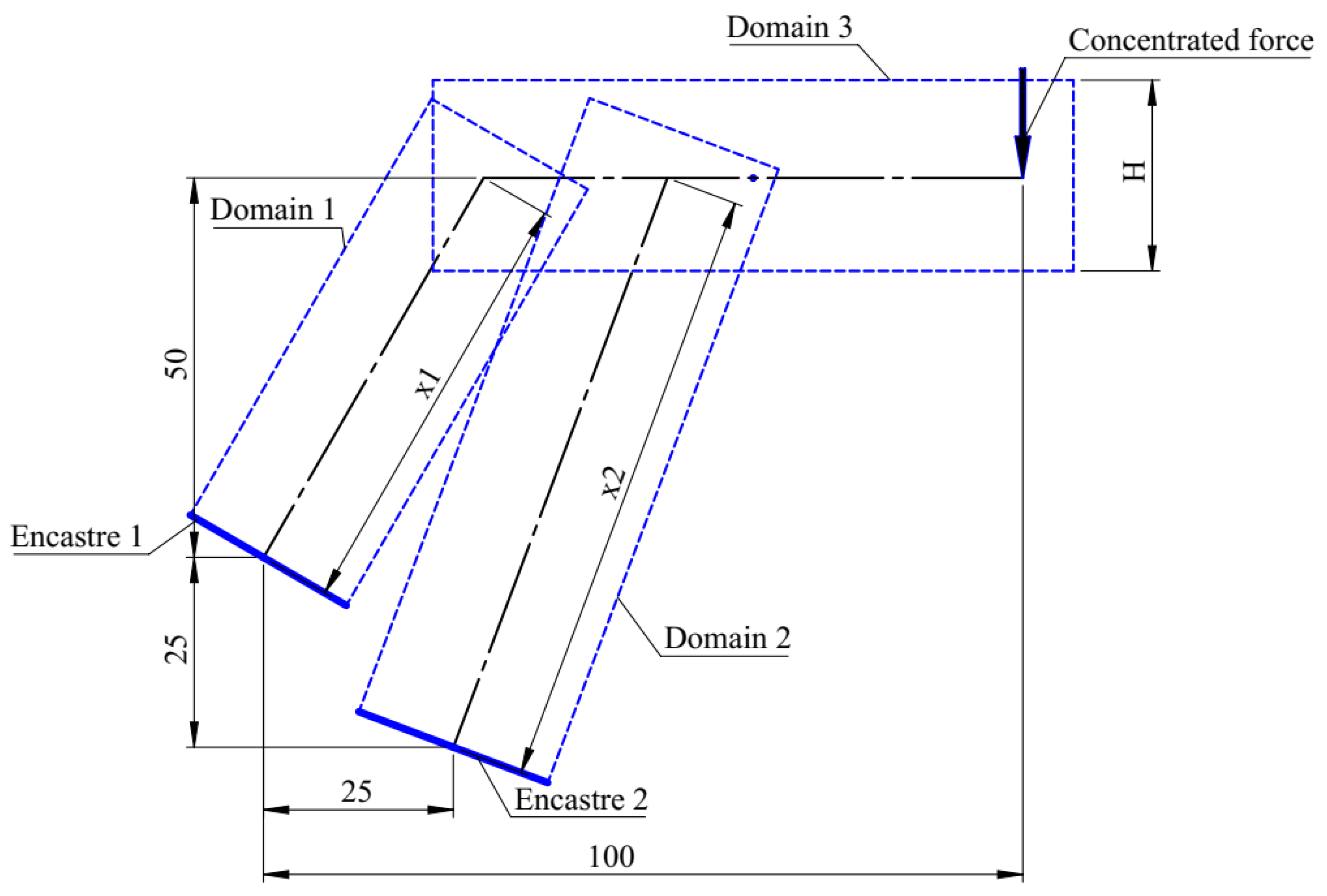
A relatively simple three-body system was selected as an example case to focus on demonstrating the behaviour of the proposed optimization procedure and the impact of cost reduction strategies. Although the system had a limited number of design variables, the coupling between multi-body and topology optimization still introduced significant computational complexity, illustrating the scalability potential of the method for more complex problems. The example multi-body system used for the evaluation of the proposed method and cost reduction strategies is given in Figure 4.

The system consists of three bodies, each treated as a separate domain, connected via hinged joints (Domain 1–Domain 3, Domain 2–Domain 3). Domain 1 and Domain 2 are inclined, each anchored at one end through encastre boundary conditions (Encastre 1 and Encastre 2, respectively), while Domain 3 extends horizontally from the upper joint of Domain 1 offset by a vertical distance H and supported by Domain 2. The system is subjected to an external concentrated force applied at the free end of Domain 3. The black dashed lines within each domain represent linkage lengths, while the blue dashed outlines indicate the domain sizes used in the topology optimization. The figure highlights the decomposition of the system into separate domains, allowing for independent yet interconnected optimization, ensuring a globally optimized structural configuration.

The outlined model serves as an input for the multi-objective optimization with nested topology optimization. The macrogeometry of the system, including lever lengths, joint locations, and load positions, is optimized using a multi-objective genetic algorithm, while the microgeometry of each domain is refined using topology optimization to minimize compliance and material usage. The response of the system is computed through equilibrium equations, accounting for the interactions between the domains via reaction forces and degrees of freedom constraints. The complete mathematical model along with all the MATLAB codes used to obtain the results can be found in the Supplementary Materials, with file test_case.m containing all the joint positions and lever lengths.

Equilibrium equations were used to devise the relations between the bodies. Finally, the optimization problem was formulated as follows:

$$\begin{array}{l}\underset{x\in {ℝ}^3}{\min }\left(f_1\left(x\right),f_2\left(x\right)\right)\\ \begin{array}{l}\begin{array}{lll}\mathrm{subjected} \mathrm{to}:\hfill & K_i{U}_i-F_i=0\hfill & i=1,\dots ,3\hfill \\ & V_i(y_i)-v_i\cdot V_{\Omega i}=0\hfill & i=1,\dots ,3\hfill \end{array}\hfill \\ \begin{array}{ll}\mathrm{where}: \hfill & f_1(x)={\displaystyle \frac{v_1\cdot N_1+v_2\cdot N_2+v_3\cdot N_3}{N_1+N_2+N_3}}\hfill \\ & f_2(x)=c_1\left(y_1\right)+c_2\left(y_2\right)+c_3\left(y_3\right);\hfill \\ & x=\left[\begin{array}{lllll}{v}_1\hfill & v_2\hfill & v_3\hfill & L_1\hfill & L_2\hfill \end{array}\right]\hfill \end{array}\hfill \end{array}\end{array}$$

(2)

where the variables correspond to those introduced in Equation (1). Moreover, indices 1, 2, and 3 correspond to Domains 1, 2, and 3, respectively.

Finally, the constraints were as follows: the volume fractions v₁, v₂, and v₃ ranged between 0.3 and 0.5; lever L₁ length ranged between 65 and 75; and the lever L₂ length ranged between 85 and 100.

5. Results and Discussion

Computational cost was evaluated using the time needed to carry out the calculations. The optimization was carried out according to the proposed procedure, resulting in Pareto-optimal fronts including all the sets of optimal solutions. The results obtained using Strategies I and II were compared to the results obtained by running the optimization procedure without any mesh coarsening or number of iterations of the topology optimization algorithm. Results obtained in this way are referred to as “reference” in the continuation of this section.

Further, it should be noted that the Pareto fronts obtained in this paper were evaluated using the hypervolume indicator [34,35], a measure that calculates the area between the Pareto-optimal front and a predefined reference point in the objective space. The hypervolume indicator reflects both convergence toward the ideal solutions and the diversity of solutions along the front, with larger values indicating a better Pareto front.

Given the disparity in objective ranges, all Pareto fronts were normalized to a common scale [0, 1] using min–max normalization to enable fair comparison. Finally, the hypervolume was calculated by linearly connecting the discrete Pareto points and measuring the area dominated up to the chosen reference point. A point slightly worse than the nadir point was used as the reference point R(1.1, 1.1) [36].

$$f_1={\displaystyle \frac{f_1^{*}-f_{1\min }}{f_{1\max }-f_{1\min }}};\hspace{1em}{f}_2={\displaystyle \frac{f_2^{*}-f_{2\min }}{f_{2\max }-f_{2\min }}}$$

(3)

where f₁^* and f₂^* denote the original values on the Pareto-optimal front, and f_1min and f_2min denote the lowest values of the volume ratio of the multi-body system and the total compliance across all Pareto fronts, respectively. Finally, f_1max and f_2max denote their maximum values and are defined analogously to f_1min and f_2min.

5.1. Resulting Pareto Fronts

Figure 5 shows the evolution of Pareto-optimal solutions across four selected generations (5th, 10th, 15th, and 20th generations) for the Reference, Strategy I, and Strategy II optimization approaches. The solutions with rather high compliance were outliers and were not shown in the figure for clarity. In all the figures, the horizontal axis represents the average volume fraction, while the vertical axis is the sum of compliances. The Reference strategy defines a well-developed Pareto front in 5th generation, while Strategy I and Strategy II significantly deviate, particularly for higher compliance values. This is due to both alternative strategies still being in the early exploration phases, as intended, providing a lower number of quality solutions.

As the generations progress, in the 10th and 15th generations, the solutions from Strategy I and Strategy II move closer to the Reference Pareto front, indicating gradual convergence. It should be noted that initial search period (coarsest mesh/lowest number of TO iterations) for both strategies occurs until reaching the 10th generation. Strategy II demonstrates a more structured evolution, aligning better with the Reference front compared to Strategy I, which still shows dispersion at higher compliance values.

Linear mesh refinement and number of TO iterations lasts until reaching generation 20. By the 20th generation, both Strategy I and Strategy II closely approach the Reference set, suggesting that the optimization process has reached a stable state. Strategy II achieves better overall alignment with the Reference front, particularly in the lower compliance region, while Strategy I has more scattered solutions, indicating a slower convergence rate. This trend suggests that Strategy II is more effective in finding high-performance solutions earlier in the optimization process, while Strategy I requires more iterations to achieve similar performance levels.

Overall, the progressive improvement in solution quality for both alternative strategies is evident, with Strategy II demonstrating superior convergence behaviour and Pareto-optimality compared to Strategy I. The final generations indicate that while all three strategies ultimately yield comparable results, their convergence rates and efficiency in identifying optimal solutions differ significantly.

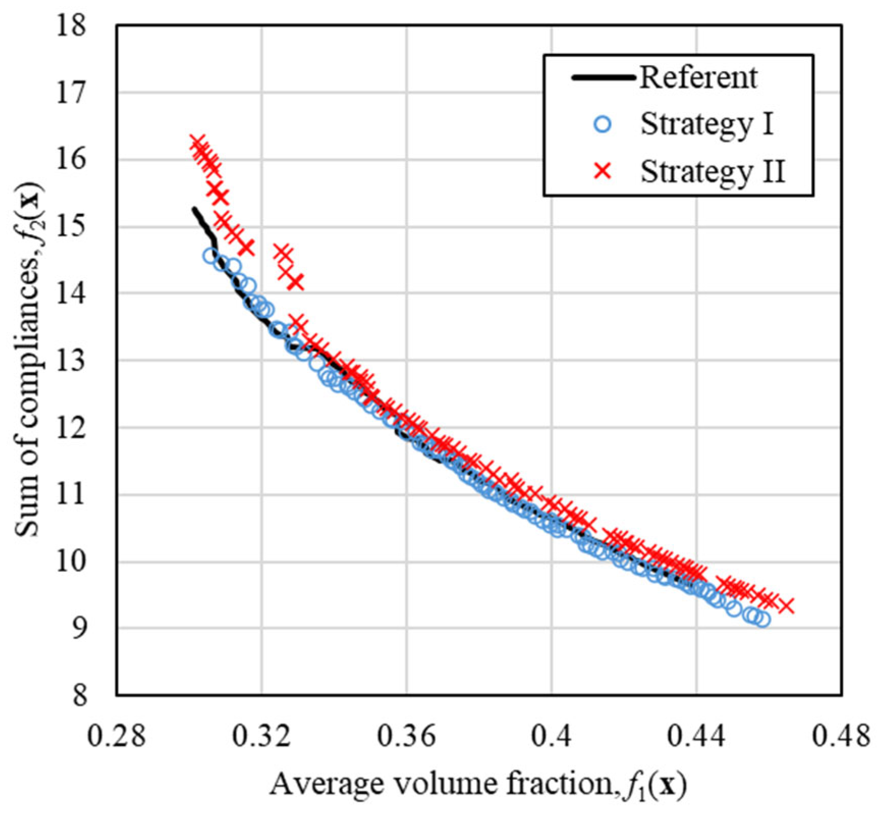
Outputs obtained after running the optimization procedure for n_gen = 25 generations using Strategy I and Strategy II were compared to the Reference set in Figure 6. By the final generation, Strategies I and II converged to the Reference Pareto front. Strategy I solutions are more evenly distributed along the Pareto front, aligning well with the Reference solutions, especially in the lower compliance regions. This suggests that Strategy I has effectively found a balanced set of solutions that optimize both stiffness and material usage. Strategy II exhibited slightly more scatter, particularly in the mid-to-high compliance range, indicating minor deviations and possibly a slower convergence rate compared to Strategy II.

Overall, this final generation confirms that all three strategies ultimately achieve comparable Pareto-optimal solutions, albeit through different optimization pathways. The results obtained using Strategy I practically match those obtained using the Reference settings; at some points the Pareto front even provides better solutions. Such behaviour is due to the inherent stochastic nature of the genetic algorithms. The Strategy II results, on the other hand, yielded lower-quality points along the Pareto-optimal front, especially for designs with lower volumes.

For the Reference set, values of objective functions f₁(x) and f₂(x) ranged from 0.3 to 0.438 and 9.685 to 15.27, respectively. For solutions obtained using Strategy I, f₁(x) ranged between 0.3 and 0.458 and f₂(x) between 9.137 and 86.9. Finally, Strategy II solutions had objective function values f₁(x) between 0.3 and 0.465 and f₂(x) between 9.342 and 25.22.

5.2. Hypervolume Indicator Values and Computational Time

The HI values for Pareto fronts are given in

Table 1. Hypervolume indicator values and computational times.

Generation No.	Reference	Strategy I	Strategy II
5	2.027	1.221	1.540
10	2.039	1.170	1.688
15	2.074	1.498	1.891
20	2.177	1.605	1.924
25	2.181	2.112	2.133
Computational time	42,226 s	16,814 s (−60.2%)	21,674 s (−48.67%)

. The results of the normalized HI analysis reveal differences in how each optimization strategy behaved across generations. The Reference case consistently achieved the highest hypervolume values, starting at 2.027 (5th generation) and gradually increasing to 2.181 (25th generation). Such a steady improvement indicated that it maintained a strong balance between the objectives. Further, its gradual increase suggests that early-stage decisions strongly influenced the long-term performance, with refinements continuing throughout the optimization process.

In contrast, Strategy I initially performed the worst, with the lowest hypervolume values of 1.221 and 1.170 at the 5th and 10th generation, respectively, indicating poor results in early generations. Such behaviour is due to using coarse mesh during the first 10 generations, which resulted in less-refined results. A significant improvement occurs after 15th generation (1.498), with further increases at the 20th generation (1.605) and 25th generation (2.112). By the final generation, Strategy I nearly matched the Reference solution, demonstrating that it can provide high-performance solutions. Such a rapid increase in the quality of solutions between 20th and 25th generation implied that using the coarse mesh helped to seed units in a quality and useful manner (only generations 20 to 25 were ran in a fully refined mesh) compared to the Reference set, which had a value of 2.027 after five generations of optimization using fully refined mesh.

Strategy II outperformed Strategy I in early generations, achieving higher hypervolume values at the 5th generation (1.540) and 10th generation (1.688). However, its improvement rate slowed in later generations, allowing Strategy I to surpass it by the 25th generation (2.133 vs. 2.112). This suggests that Strategy II provided better results in its early exploration but lacked the refinement needed to sustain its advantage in later iterations. By the 25th generation, all three strategies achieved similar normalized HI values, indicating that despite different optimization approaches, all strategies ultimately converged to solutions of comparable efficiency in the normalized objective space. The Reference solution provided the best results, while Strategy I demonstrated the most improvement, and Strategy II yielded strong early solutions but struggled to refine them.

Computational times were obtained for each case using the tic and toc MATLAB functions. The time elapsed to obtain the Reference set was 42,226 s, which was reduced to 16,814 s and 21,674 s when using Strategy I and Strategy II, respectively. Thus, Strategy I reduced the computational time by 60.2% and Strategy II reduced it by 48.67%, implying significant savings in necessary resources.

After accounting for both the quality of solutions on Pareto fronts and the associated computational costs, it was found that Strategy I provided the most balanced outputs. It provided high-quality solutions, nearly comparable to those found via the Reference strategy, at only a fraction of the computational time.

Finally, the stochastic nature of evolutionary algorithms should be commented on, as it introduces slight variability between optimization runs. The variations caused by the use of random variables during the optimization are mitigated via replications, i.e., repeated tests. The repeated tests indicated stable convergence patterns and minimal variation. However, future work on the subject ought to incorporate formal statistical analyses to comprehensively quantify robustness and repeatability.

5.3. Optimized Structures

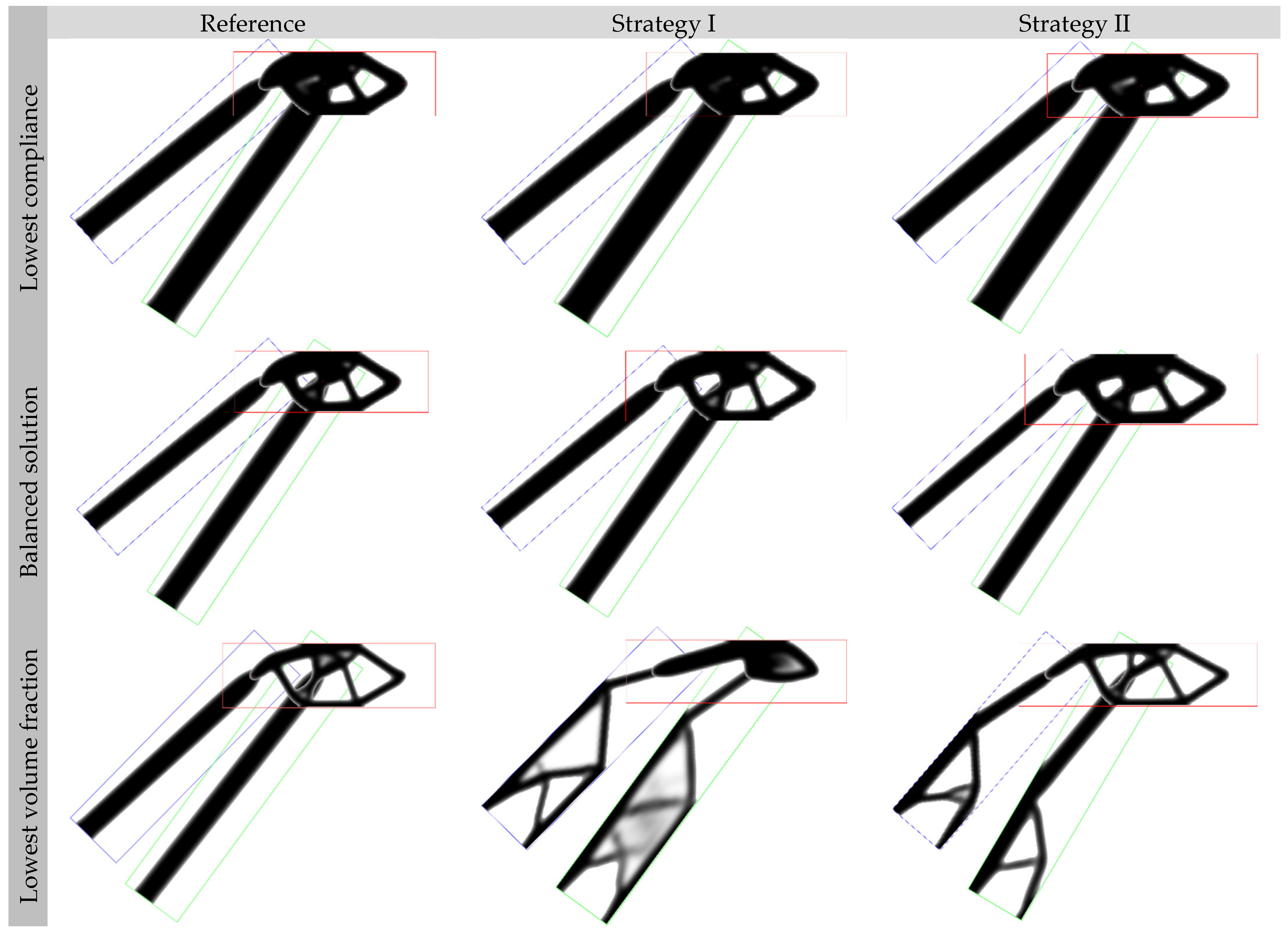
To better illustrate the structures obtained for the example case, a total of nine solutions were selected from Pareto-optimal fronts—three for each of the strategies. Among the three, solutions with the lowest compliance, lowest volume fraction, and the balanced solution (50th solution on the Pareto front of the 100 in total) were selected. The selected structures are shown in Figure 7, where Domain 1 has blue borders, Domain 2 has green borders, and Domain 3 has red borders. The solutions with the lowest total compliance were nearly identical, regardless of the applied computational cost reduction strategy. Similar behaviour was observed for balanced solutions (Figure 7, 2nd row). In these, the parts described by Domain 1 and Domain 2 were straight levers; the multi-objective optimization ensured that said parts were positioned to ensure only compressive/tensile loads.

When considering solutions with the lowest volume fraction, the Reference approach followed the same principle, selecting continuous thick beams. On the other hand, a greater variety of solutions was obtained when using Strategy I or Strategy II. The Strategy I low-volume solution comprises a short and thick Domain 3 part, while Domain 1 and Domain 2 had parts with lattice structures. It can also be seen that Domain 2 (green) did not converge, as evidenced by grey areas. The Strategy II solution also included lattice structures for all three domains, with the Domain 3 solution shape being similar to those of higher-volume solutions (rows 1 and 2 of Figure 7).

6. Conclusions

In this study we introduced an optimization approach comprising multi-objective and topology optimization. The approach enables the simultaneous optimization of multi-body structures by refining both support and joint locations and internal material distribution. The sum of compliances and the overall material volume fraction were used as objective functions for an example multi-body system. Further, two strategies were developed to address the computational cost challenges associated with running multiple topology optimizations per unit within the multi-objective optimization algorithm. Strategy I uses coarser mesh in early generations, gradually refining it as the multi-objective algorithm converges. Strategy II decreases the number of topology optimization algorithm iterations in early generations, progressively increasing it in later stages of the optimization process.

In the case study addressed, the results demonstrated that both strategies significantly reduced the computational time compared to the Reference set obtained with no reductions, while achieving similar Pareto-optimal solutions. Strategy I reduced the computational time by 60.2%, while Strategy II achieved a 48.67% reduction. Hypervolume indicator (HI) values were calculated for each of the three strategies, showing that all three ultimately converged to comparable HI values, with Strategy I showing the most improvement in later generations. It should be added that Pareto front values were normalized prior to calculating the HI values to prevent one objective from dominating the hypervolume calculation. Among the two strategies, Strategy I demonstrated the most balanced trade-off between efficiency and solution quality, closely matching the performance of the Reference method. Finally, it should be noted that conclusions were made based on the observed case. Hence, additional research is needed to explore whether these observations hold for a generalized case with diverse multi-body systems, and to provide mathematical validation of their applicability across different scenarios.

The primary limitations of this study include the lack of dynamic optimization, as the proposed method is currently limited to static loading conditions. Additionally, the study is confined to 2D structures, and while theoretically extendable to 3D cases, associated challenges are yet to be addressed. The extension of the proposed methodology to 3D problems involves increased computational complexity due to a higher number of DOFs, more complex meshing requirements, and greater computational load per iteration. Future work should address these challenges by employing advanced computational techniques such as parallel processing or surrogate modelling. Finally, the scalability of the genetic-algorithm-based optimization should be further examined for larger, more complex problems, as alternative methods like surrogate models or hybrid metaheuristics may offer better performance. However, it provides an important first step for addressing the aforementioned problems.

The proposed optimization framework is feasible for integration into standard CAD/CAE workflows, primarily for preliminary design optimization. However, as noted earlier, practical applications for complex 3D scenarios may encounter an exponential growth in computational costs.