Abstract
The accurate estimation of the remaining useful life (RUL) of lithium-ion batteries (LIBs) is essential for ensuring safety and enabling effective battery health management systems. To address this challenge, data-driven solutions leveraging advanced machine learning and deep learning techniques have been developed. This study introduces a novel framework, Deep Neural Networks with Memory Features (DNNwMF), for predicting the RUL of LIBs. The integration of memory features significantly enhances the model’s accuracy, and an autoencoder is incorporated to optimize the feature representation. The focus of this work is on feature engineering and uncovering hidden patterns in the data. The proposed model was trained and tested using lithium-ion battery cycle life datasets from NASA’s Prognostic Centre of Excellence and CALCE Lab. The optimized framework achieved an impressive RMSE of 6.61%, and with suitable modifications, the DNN model demonstrated a prediction accuracy of 92.11% for test data, which was used to estimate the RUL of Nissan Leaf Gen 01 battery modules.
1. Introduction
This an extended version of the “Accurate Prediction of Remaining Useful Life for Lithium-ion Battery Cells Using Deep Neural Networks” conference paper published by IEEE [1]. The commercialization of lithium-ion battery technology by Sony in 1991 was a significant milestone given the increasing demand for sophisticated energy storage systems that primarily depend on technology, mobility, and energy efficiency [2]. Due to their comparatively high energy and power density, remarkable efficiency, low self-discharge rate, and extended lifespan [3,4] compared to other batteries, LIBs have since found extensive applications in a variety of industries, including electric vehicles, household appliances, communication applications, aerospace, cell phones, and other fields [5]. The main energy source for the most recent iterations of the Tesla, Chevrolet Volt, Nissan Leaf, and BYD E6 is lithium-ion batteries.
As lithium-ion batteries continually experience cycles of charge and discharge, their overall capacity gradually reduces—a process known as “health degradation”. This aging process is influenced by various aspects. As the lithium ions migrate between the anode and cathode and induce capacity fading, a solid layer known as the Electrolyte Interface (SEI) layer repeatedly forms on the electrode’s surface. Another factor is lithium plating, which occurs when a battery is overcharged in cold conditions, turning lithium ions into lithium metal. Additionally, capacity degradation is brought on by an increase in internal impedance [3,4,6].
Because LIBs deteriorate, safety and dependability have become increasingly important; battery failures can harm an entire system and potentially result in serious injuries and considerable financial losses. An explosion or fire may result from a lithium-ion battery malfunction in electric vehicles [7]. The RUL is a crucial indicator that supports safety concerns and is used to assess the dependability of electronic systems and optimize LIB performance [3]. Complex degradation mechanisms, noisy operation settings, and capacity regeneration noise pose challenges to RUL prediction [8].
A lithium-ion battery’s remaining usable life (RUL) is expressed as the number of cycles left before the capacity decreases to less than 70% of its initial capacity [9].
In recent years, significant advancements have been made in the field of RUL prediction, particularly through the application of deep learning (DL) techniques. Models such as Convolutional Neural Networks (CNNs), Recurrent Neural Networks (RNNs), Long Short-Term Memory (LSTM), Gated Recurrent Units (GRUs), and Transformer architectures have been widely adopted to capture complex degradation patterns and temporal dependencies in lithium-ion batteries [10,11,12]. Attention mechanisms and hybrid models combining physics-based and data-driven approaches have also emerged to enhance prediction robustness and accuracy. In parallel, research on battery safety has focused on identifying failure modes such as thermal runaway, overcharging, and internal short circuits, and integrating early warning systems into battery management systems (BMSs). DL-based anomaly detection and safety-aware RUL prediction models are being explored to address these concerns. Despite these advancements, challenges remain in practical implementation, including model interpretability, generalization across different battery chemistries and usage patterns, data scarcity for extreme conditions, and computational constraints for real-time deployment. Addressing these issues is critical for the development of reliable and safe DL-based RUL prediction systems suitable for real-world applications [13].
Because of this, estimating RUL is still crucial, and there is currently no totally accurate way to anticipate RUL. The goal of this study is to combine an autoencoder with Deep Neural Networks (DNNs) that use memory features in order to create an accurate prediction model that addresses these problems. Using previous data on battery health, operating conditions, and degradation patterns—which offer practical insights for optimizing battery usage and maintenance strategies—the model will learn to estimate the RUL effectively. The project advances the creation of sophisticated battery management systems that facilitate more effective use and increase the longevity of lithium-ion batteries across a range of applications.
Model-based and data-driven methods are the two categories into which the approaches to RUL prediction can be divided [10]. Model-based methods rely on comparable circuit models, dynamic models, and electrochemical concepts. Despite the great accuracy of model-based strategies, data-driven approaches have garnered significant attention [10] because of their limited applications and complexity [3]. Nevertheless, the accuracy of these machine learning models is rather moderate [3].
- (A)
- Related work
- (1)
- Model-Based Approach
The models are computationally sophisticated and follow a stringent structure tailored to a particular framework. Xu and Chen estimated the RUL of LIBs by developing a state–space model, also referred to as a dynamic model [14]. The model parameters and states are refined through the integration of expectation maximization (EM) and the Extended Kalman Filter algorithm. Heng et al. propose an enhanced approach for forecasting the remaining useful life of LIBs by leveraging an improved unscented particle filter (UPF) algorithm combined with linear-optimizing combination resampling [11].
- (2)
- Data-Driven Approach
The data-driven method, in comparison to the model-based approach, is faster, less complex, and more convenient. Zhang et al. introduced a technique for estimating the remaining useful life (RUL) based on the Box–Cox transformation (BCT), a statistical method typically applied in Linear Regression and Time Series Analysis to stabilize variance and normalize the data distribution [15]. They leveraged this technique in predicting the RUL of lithium-ion batteries (LIBs). Similarly, Nuhic et al. employed Support Vector Machines (SVMs) to diagnose and predict system health, particularly focusing on estimating the state of health and RUL of LIBs [16]. However, due to the inherent limitations of SVM models, such as the requirement for the Kernel Function to satisfy Mercer Conditions, calculating the loss function can be challenging.
Currently, researchers are exploring Neural Network (NN)-based models, including Deep Neural Networks (DNNs) and Recurrent Neural Networks (RNNs) with Long Short-Term Memory (LSTM) [10,12]. Zhang et al. utilized LSTM to predict the RUL of LIBs [11]. Although RNN and LSTM models demonstrate superior accuracy compared to other machine learning models, they present certain challenges, including high computational requirements, significant memory consumption, and extended training times [17]. Additionally, implementing dropouts in LSTM models is complex.
To mitigate these challenges, we introduced a deep learning approach that integrates memory-based features, which have been rarely explored in the literature. Given the degradation patterns observed in LIBs, these patterns can be harnessed for Time Series Analysis, allowing memory-based features to be incorporated into the model. In this study, we prioritized feature engineering and proposed an optimized model architecture to enhance accuracy. The proposed method was benchmarked against SVM and Linear Regression models.
The novelty of this paper lies in utilizing auto-encoded memory features integrated with a Deep Neural Network (DNN) for the accurate prediction of remaining useful life (RUL). This approach is applied to real-world field data collected from Nissan Leaf batteries, demonstrating the model’s practical effectiveness. Additionally, the novelty of this project lies in its ability to predict the RUL of a Nissan Leaf Gen 1 battery module, which shares similar charge–discharge characteristic graphs with the model’s trained dataset. This is achieved by performing the charge–discharge process while maintaining key factors consistent with the training dataset. Furthermore, we introduce a novel data normalization method, enabling comparisons to be made between lithium-ion batteries with different capacities. Notably, this method has been applied to real-world data, showcasing its utility in practical applications, such as predicting the RUL of Nissan Leaf car batteries, even in the absence of structured or consistent charge patterns.
2. Materials and Methods
2.1. Proposed RUL Prediction Approach
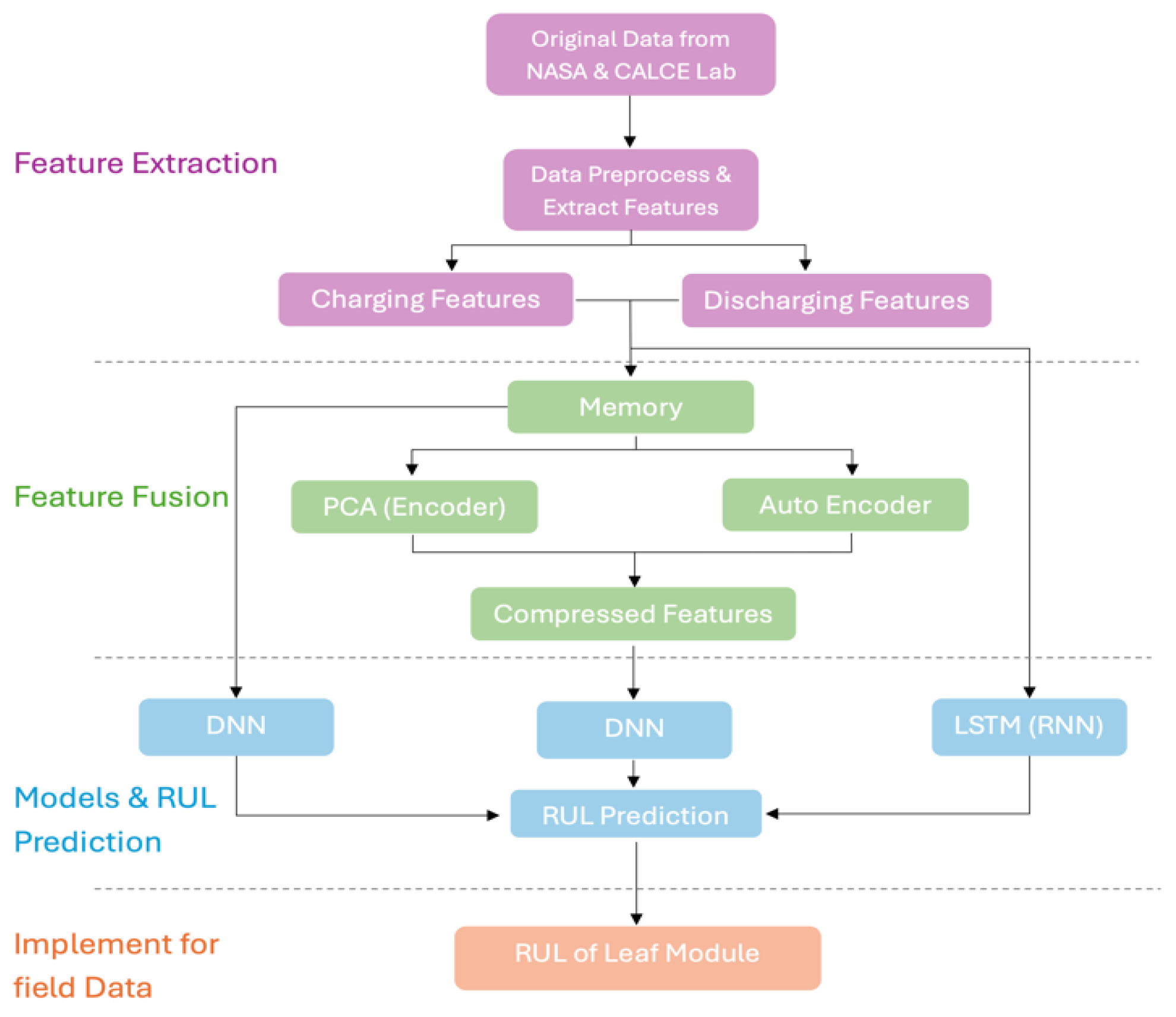
The suggested model framework for predicting the RUL is shown in Figure 1. Initially, the original data’s insightful properties were retrieved, exposing important trends and patterns that might be used to predict the batteries’ RUL.
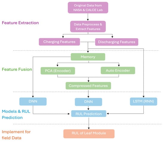
Figure 1.
Proposed Methodology.
After that, a PCA with memory feature integration was used to complete feature fusion. In order to forecast the RUL as the output, the encoded features were finally given into the DNN model.
- Dataset (Original Signal)
A set of four lithium-ion batteries (B0005, B0006, B0007, and B0018) from the NASA dataset were subjected to three distinct operational profiles: charge, discharge, and impedance, all conducted at room temperature. These batteries were selected for predicting the remaining useful life (RUL). The NASA dataset provides time series data for each charge and discharge cycle, including measurements of voltage, current, temperature, and impedance. Each cycle follows the widely adopted constant current–constant voltage (CC-CV) pattern for both charging and discharging.
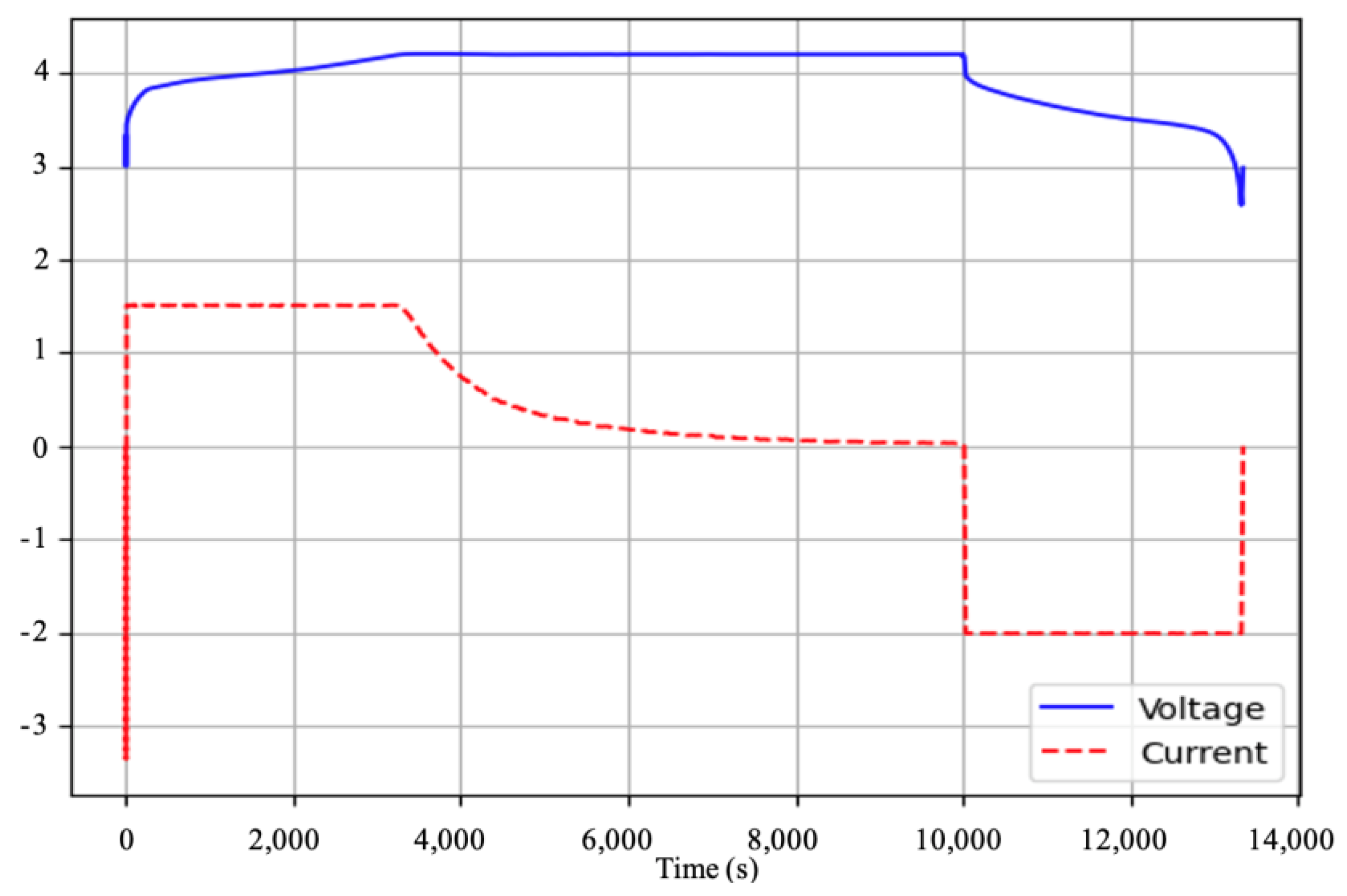
The testing process was repeated until the battery capacity degraded to 70% of its initial value. A complete cycle comprises both a charge and a discharge sequence. Figure 2 illustrates a typical charge–discharge cycle of a lithium-ion battery. All charge–discharge cycles were compared against this reference pattern and those that deviated significantly were excluded from the dataset, as such anomalies could negatively impact the performance of the neural network.
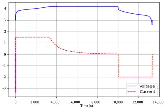
Figure 2.
Typical complete cycle of a lithium-ion battery.
- Charging process: Initially, the battery is charged with a constant current (CC) until the voltage is raised to a maximum upper limit. Then, the voltage is kept constant (CV) while the current drops to a certain lower limit.
- Discharging process: The entire discharge process is at a constant current (CC) of a specific value until the voltage drops to a certain lower limit.
- B.
- Feature Extraction
In Deep Neural Networks, feature engineering plays a pivotal role in the success of prediction models, especially in complex scenarios like battery life prediction. The dataset gathered from charging and discharging cycles of batteries presents a significant challenge: the number of data points varies across cycles, with some having as few as 800 data points and others as many as 5000. This disparity makes it impractical to directly feed raw data into the neural network, necessitating data preprocessing and feature extraction to ensure consistent and meaningful input.
Feature extraction is crucial because, in theory, incorporating a broader set of features enhances the model’s accuracy. A well-structured representation of the data is essential for identifying trends and key features that contribute to better predictions.
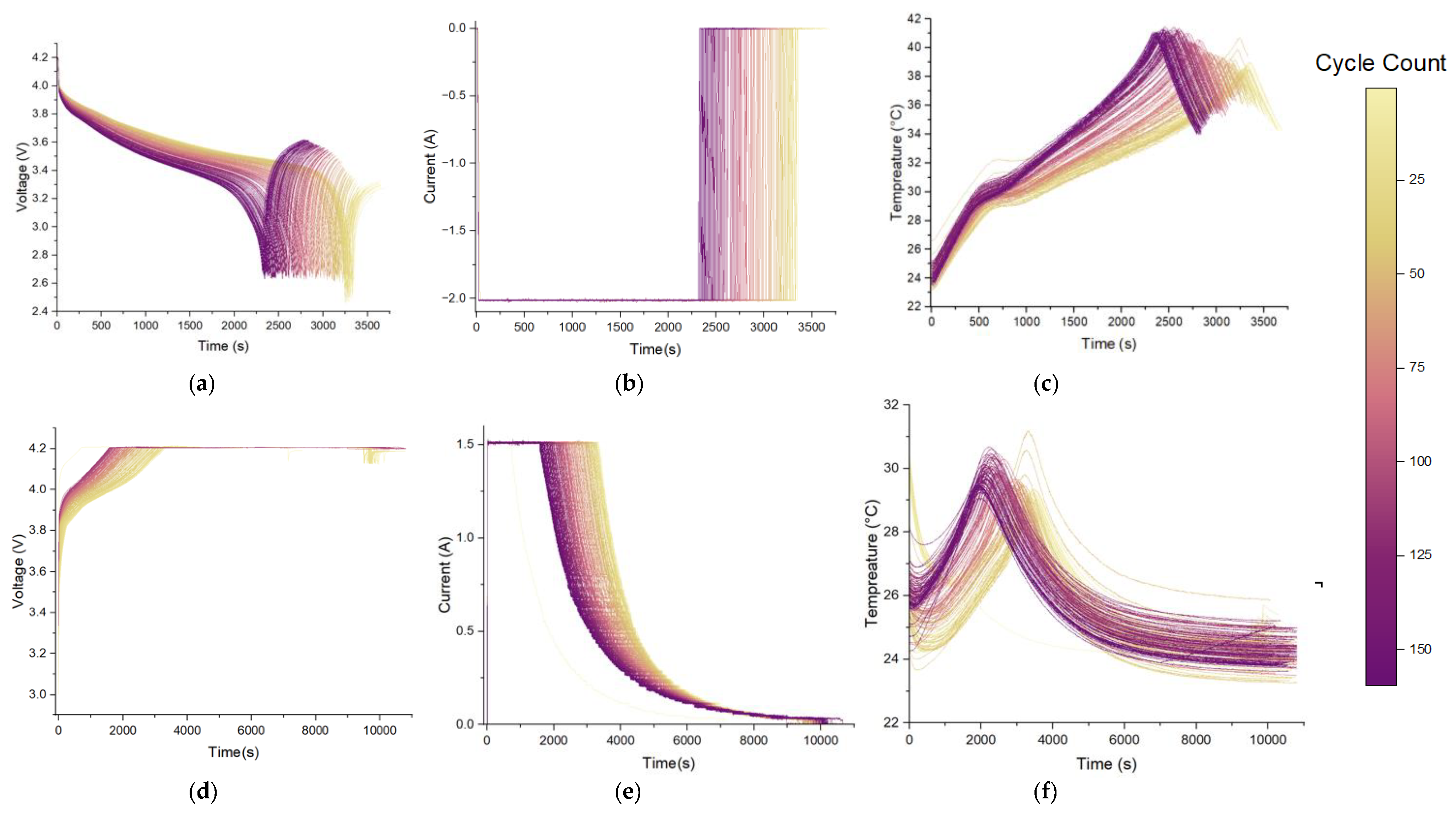
As batteries undergo repeated charge and discharge cycles, they degrade due to several mechanisms, including the loss of active lithium ions, lithium plating, electrode degradation, metal dissolution, and an increase in internal impedance [18]. These factors lead to a reduction in the battery’s capacity over time. Consequently, time series data of current, voltage, and temperature during charging and discharging cycles reveal distinct patterns when analyzed against the cycle count.
For instance, the figures for a B0005 battery, depicted in Figure 3, illustrate the variation in voltage, current, and temperature of the battery cell B0005 over time during the charging and discharging processes across multiple cycles. Figure 3a–c corresponds to the discharge cycles while Figure 3d–f corresponds to the charge cycles. By analyzing these curves, it is evident that certain parameters of lithium-ion batteries are highly sensitive to the cycle count and exhibit clear trends. For instance, Figure 3a highlights whether all discharging cycles follow a typical pattern, as shown in Figure 2, and highlights how the time taken to reach the minimum terminal voltage decreases as the cycle count increases. Similarly, Figure 3e highlights how the constant current (CC) charging time shortens with each successive cycle.

Figure 3.
B0005. (a) Discharging voltage vs. time; (b) discharging current vs. time; (c) discharging temperature vs. time; (d) charging voltage vs. time; (e) charging current vs. time; (f) charging temperature vs. time.
These characteristic features, extracted from the original data for each cycle, serve as critical inputs for predicting the battery’s remaining useful life (RUL). Identifying and leveraging these features enables the neural network to make more accurate and reliable predictions.
These distinguishing characteristics were taken from the original data for every battery cycle in order to forecast the RUL. While plotting each cycle for each battery, we observed errors in some battery cycles, such as missing data points and graphs showing abnormalities compared to others. These cycles were skipped during model training to prevent potential errors in the model. However, some of these cycles were retained to evaluate the model’s accuracy. The following features are extracted from the charging and discharging operation.
Charging Features:
Upper Cut-off Voltage Time
(tmin(i), Vi), Vi ≥ Upper Cut off Voltage, i = 1, 2, 3, … where tmin(i) represents the time when the battery terminal voltage reaches the maximum value first and Vi represents the value of output voltage in the ith cycle.
Constant Current Charging Time (CCCT)
(tmin(i), Ai), Ai ≤ Constant Current Value, i = 1, 2, 3, … Ai represents the value of the current value in the ith cycle.
Constant Voltage Charging Time (CVCT)
(tmin(i), Vi), Vi £ Constant Voltage Value, i = 1, 2, 3, … where Vi represents the value of the output voltage in the ith cycle.
Maximum Charging Voltage Time
The time required to reach the maximum battery-measured voltage. (tmax, Vmax) = {(ti, Vi| max(Vi))}, i = 1, 2, 3, …, m, where tmax is the time stamp for which the maximum voltage Vmax is measured in the ith cycle.
Maximum Temperature Time
Time when the battery reaches its maximum temperature. (tmax, Tmax) = {(ti, Ti| max(Ti))}, i = 1, 2, 3, …, m, where tmax is the time stamp for which the maximum temperature Tmax is measured at the ith cycle
Area Under Voltage Curve
Area covered by the voltage vs. time curve.
Area Under Current Curve
Area covered by the current curve vs. time.
Maximum Power Time
(tmax, (V*I)max) = {(ti, V*I| max(V*I))}, i = 1, 2,…, m, where the tmax is the time stamp for which the maximum current and voltage product is measured at the ith cycle.
Discharging Features:
Discharging Time
During the discharging process, the time for which the battery terminal voltage reaches its minimum voltage.
Maximum Temperature Time
Time which gives the maximum temperature at the discharging process for each cycle.
Area Under Voltage Curve
Area covered by the voltage measured vs. time plot.
Area Under Current Curve
Area covered by the current vs. time plot.
Discharging Capacity
The remaining capacity at each discharging cycle.
When combining the charge cycle and discharge cycle, there are 13 features for one cycle.
- C.
- Generating Labels and Data Normalization
For the training phase of the RUL prediction model, correct labels are necessary after the features have been extracted from the raw data. To obtain the supervised data (xi,yi), the appropriate RUL (yi) for the ith cycle characteristics (xi) must be calculated. The ith cycle’s RUL was determined as
where L is the total count of charge and discharge cycles.
To mitigate any adverse effects resulting from varying value ranges, data normalization is an essential component of Neural Network models [19]. We used the minimum–maximum normalization technique to rescale all of the dataset’s features inside the interval [0–1]. The following is the min–max normalization formula [19].
where xmax denotes the greatest value of feature x and xmin denotes its minimum value.
By ensuring that all features have the same scale, this normalization strategy can help the neural network model perform better and coverage more quickly.
- D.
- Memory Features
Time Series Analysis can be used to characterize the patterns in the data; therefore, memory-based characteristics spanning numerous cycles—which have not been used much—can be applied here. Utilizing a window that spans many cycles, extracted features are used with memory to capture the properties seen in the preceding n cycles. By increasing the number of preceding cycles (n), testing loss was decreased.
For instance, in order to predict the RUL for the ith cycle, yi, all of the features from the previous n cycles, {xi, xi−1, xi−2, xi−3, …, xi−n}, were used in addition to the features of the current cycle, xi. Several window sizes were used to test the proposed DNN in order to increase the number of cycles (n).
- E.
- Feature Fusion
Adding memory features to the DNN model increases the number of input features, leading to potential redundancy, higher computational complexity, and inefficiency. To address this, we reduced the dimensionality of the input data using two proven techniques: Principal Component Analysis (PCA), Nonlinear PCA, and an autoencoder.
- (1)
- Principal Component Analysis (PCA)
In this project, to handle the high-dimensional dataset and reduce the risk of errors such as overfitting, we used Principal Component Analysis (PCA) as the first encoding technique. PCA simplifies the dataset by identifying new variables, known as principal components (PCs), which are linear combinations of the original features. These components retain the most significant information from the original data while reducing dimensionality. The process of applying PCA involves the following steps [20]:
Standardization: The data is standardized to ensure all features have a mean of zero and a standard deviation of one, preventing any feature from dominating the analysis.
Covariance matrix calculation: A covariance matrix is computed to measure how different features vary together, identifying relationships between them.
Eigen decomposition: The eigenvalues and eigenvectors of the covariance matrix are calculated to determine the directions (eigenvectors) with the highest variance (eigenvalues).
Selection of principal components: The principal components with the largest eigenvalues are selected, capturing the most variance and ensuring that only the most meaningful information is retained.
Projection: The original dataset is projected onto the space defined by the selected principal components, resulting in a reduced-dimensional representation of the data for further analysis. Figure 4 illustrates the original data compared with the decoded data for the case of n = 3 in PCA.
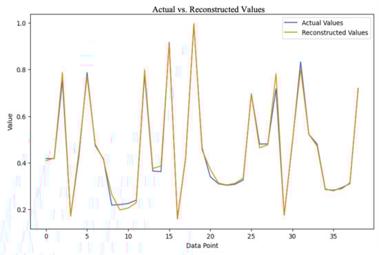
Figure 4.
Original Data vs. Decoded Data from PCA.
- (2)
- Nonlinear PCA
In this study, Nonlinear PCA was not used due to the large size of the dataset, making it computationally impractical to handle. Instead, we employed an autoencoder, which provides a scalable and efficient solution for dimensionality reduction by learning nonlinear representations of the data.
- (3)
- Autoencoder
An autoencoder is a type of neural network used for unsupervised learning, primarily for dimensionality reduction and feature extraction [21]. It aims to learn an efficient, compressed representation of input data by encoding it into a lower-dimensional space and then reconstructing it back to the original form. The autoencoder consists of two main parts:
- Encoder: Compresses the input data into a lower-dimensional latent space, capturing the most essential features.
- Decoder: Reconstructs the original data from the compressed representation, ensuring that the important information is retained.
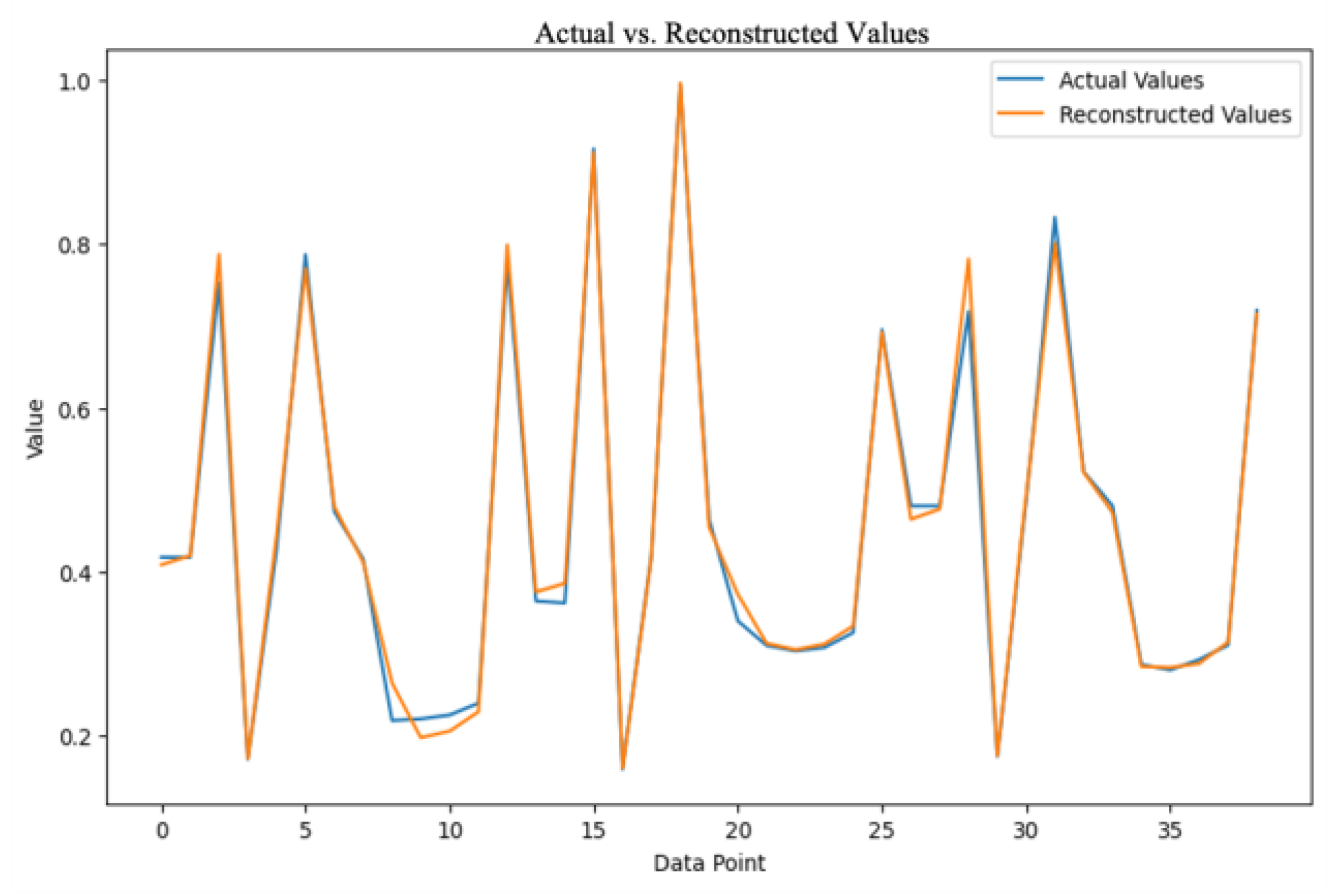
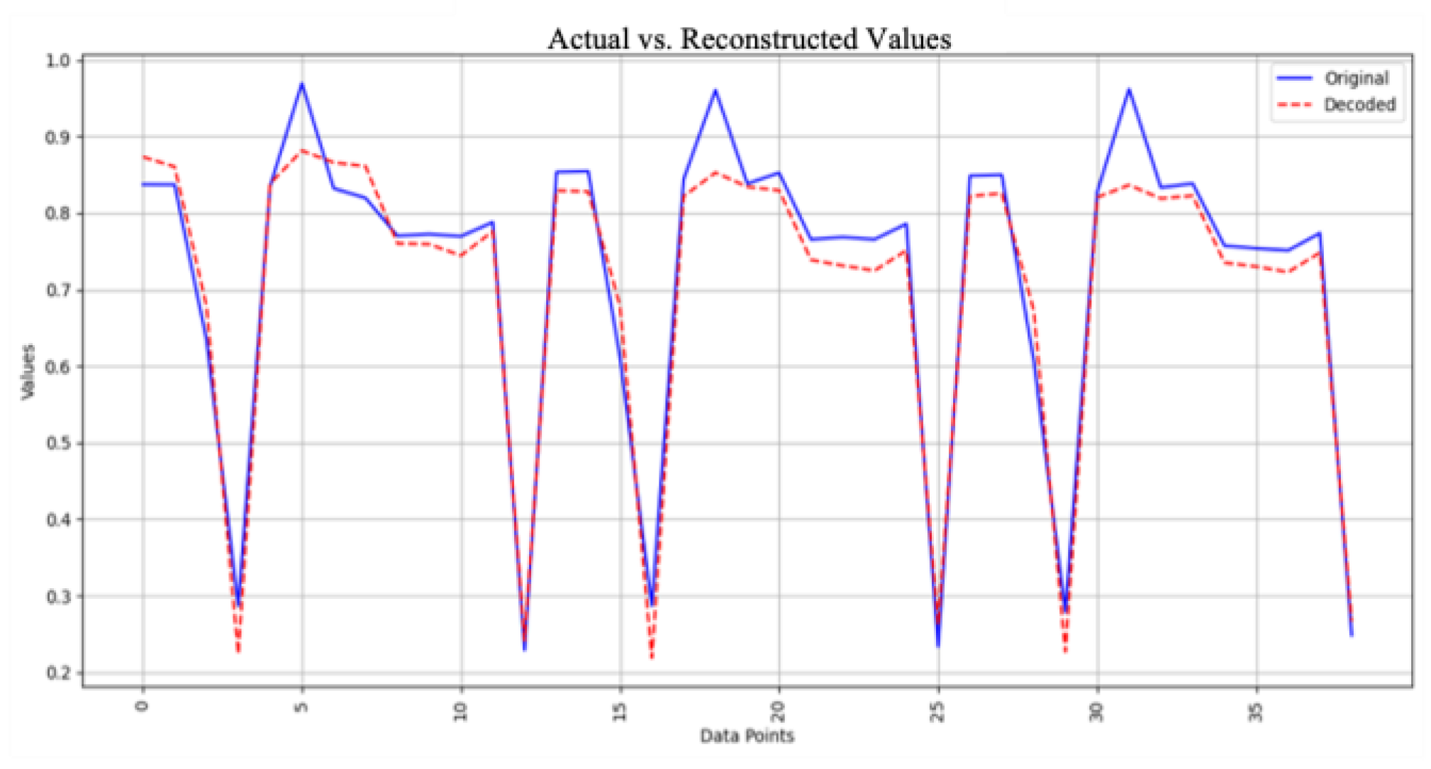
In this project, we only consider the encoder, as the encoded representation is used as input to the DNN model. The decoder is only employed to verify the accuracy of the autoencoder model by evaluating how well it reconstructs the original input. Figure 5 illustrates the original data compared with the decoded data for the case of n = 3 in the autoencoder.
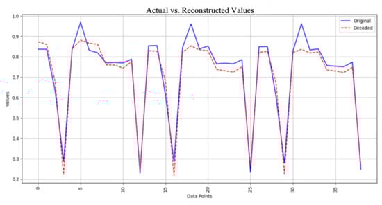
Figure 5.
Original data vs. decoded data from autoencoder.
- F.
- Training Neural Network Models with and without encoded Features
Table 1 represents the number of input features for PCA and autoencoder along with their outputs, categorized by different number of previous cycles.

Table 1.
Encoded features.
The proposed model for remaining useful life prediction is a Deep Neural Network (DNN) that leverages both current and previous cycle features. The output from the encoder serves as input to the DNN, along with the target output, as the DNN operates under a supervised learning framework. In Deep Neural Networks, each input passes through a nonlinear activation function to generate the input for the subsequent layer. The mapping in the ith layer can be expressed as follows:
where represents the nonlinear activation function, W denotes the weight matrix, and b corresponds to the bias of the ith layer.
During the training phase, the weights and bias parameters of the layers are optimized interactively to minimize the loss function, which is defined by comparing model output with the target output. After tuning the hyperparameters, the selected DNN model consists of four fully connected layers. Each layer has 10, 7, 4, and 1 neurons, respectively. The ReLU activation function is used for the hidden layers, while the sigmoid function is applied to the output layer. The model’s performance during the testing is evaluated using the Root Mean Squared Error (RMSE%) value.
2.2. Nissan Leaf Gen 01 Battery Module
- Introduction
The adoption of electric vehicles (EVs) has surged rapidly in recent years. In 2022 alone, 10.5 million new EVs and plug-in hybrid vehicles were introduced to the market. This represents a significant growth in market share, with EVs accounting for 14% of global vehicle sales in 2022, up from 9% in 2021. Projections suggest that by 2030, EVs could capture up to 35% of the market. Most EVs are powered by lithium-ion battery packs, which are composed of multiple battery modules. These batteries typically reach the end of their automotive service life after approximately 10 years. However, even after this, many still retain 60–67% of their original capacity, making them suitable for secondary applications such as energy storage systems (ESSs), particularly for solar power plants [22].
- B.
- Why Use This Model when BMSs Already Exist?
EVs are equipped with a sophisticated battery management system (BMS), which continuously monitors and estimates the remaining useful life (RUL) of the battery during operation. However, once the battery pack is removed from the vehicle and disconnected from the BMS, the system’s memory is reset and the ability to predict the RUL is lost. This presents a significant challenge when repurposing retired EV batteries for second-life applications.
Therefore, this study aims to develop a predictive model for estimating the remaining useful life (RUL) of Nissan Leaf Gen 01 battery modules after their removal from the BMS. The proposed method focuses on utilizing simple tests to predict the battery’s remaining life, ensuring the feasibility of second-life applications in energy storage systems.
- C.
- About the Battery Module
The Nissan Leaf Generation 01 battery pack consists of 48 modules connected in series, with each module comprising four lithium-ion cells. The anode material is a combination of LiMn2O4 and LiNiO2, while the cathode is composed of graphite. The configuration of each battery module is 2P2S, meaning two parallel sets are connected in series, resulting in an overall pack configuration of 2P-96S. The nominal capacity of the battery pack is 66.2 Ah (24 kWh) at a 0.3C rate, where the C-rate defines the rate of charge or discharge relative to the total capacity. For instance, a 1C rate would fully charge or discharge the battery in one hour, while a 2C rate would complete the process in 30 min. Due to high current requirements managed by the battery management system (BMS), the usable capacity is set to 65.6 Ah. Each module has an internal resistance of 1 mΩ, and the series resistance across the pack is 2 mΩ. The operating voltage range for a single cell is 2.8 V to 4.2 V, with a mean cell voltage of 3.8 V, yielding a typical module voltage of 7.6 V and a maximum module voltage of 8.4 V. Each module weighs approximately 3.8 kg, with an energy density of 213 Wh/L and a specific energy of 132 Wh/kg. Table 2 summarizes the battery module parameters.
Table 2.
Nissan Leaf Gen 01 battery specifications.
- D.
- Data Collection
- Charging Process
Due to the difference in capacity between the Nissan Leaf Gen 01 battery module and the training set, it was necessary to ensure that 1.5 A was driven through each cell. Given the 2P-2S configuration of the module, a total current of 3 A was applied during the charging process.
Charging was carried out using a RIGOL DP 932U DC power supply in constant current mode until the battery voltage reached 8.4 V. Once this voltage reached that value, the current gradually decreased while the voltage kept constant. The charging process was stopped when the current was reduced up to 40 mA.
- 2.
- Discharging Process
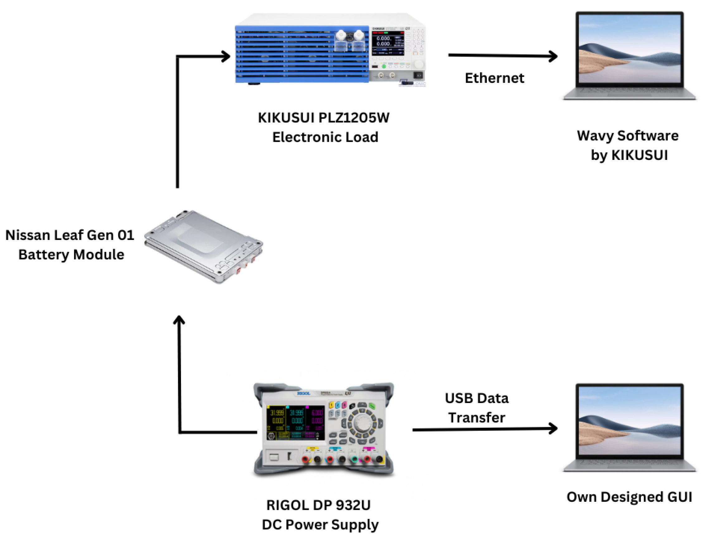
Discharging was conducted using a constant current method at 4 A, with the assumption that each cell in the module drains 2 A, consistent with the training dataset. This process was carried out using a KIKUSUI PLZ1205W electronic load. Data collection was performed using version 5.1.0 of the SD023-PLZ-5W (Wavy for PLZ-5W) software, provided by KIKUSUI.
Figure 6 illustrates the complete charging and discharging setups used in the laboratory for the data collation process for Nissan Leaf Gen 01 battery modules.

Figure 6.
Charging and discharging procedure for Nissan Leaf module.
- E.
- Data Normalization
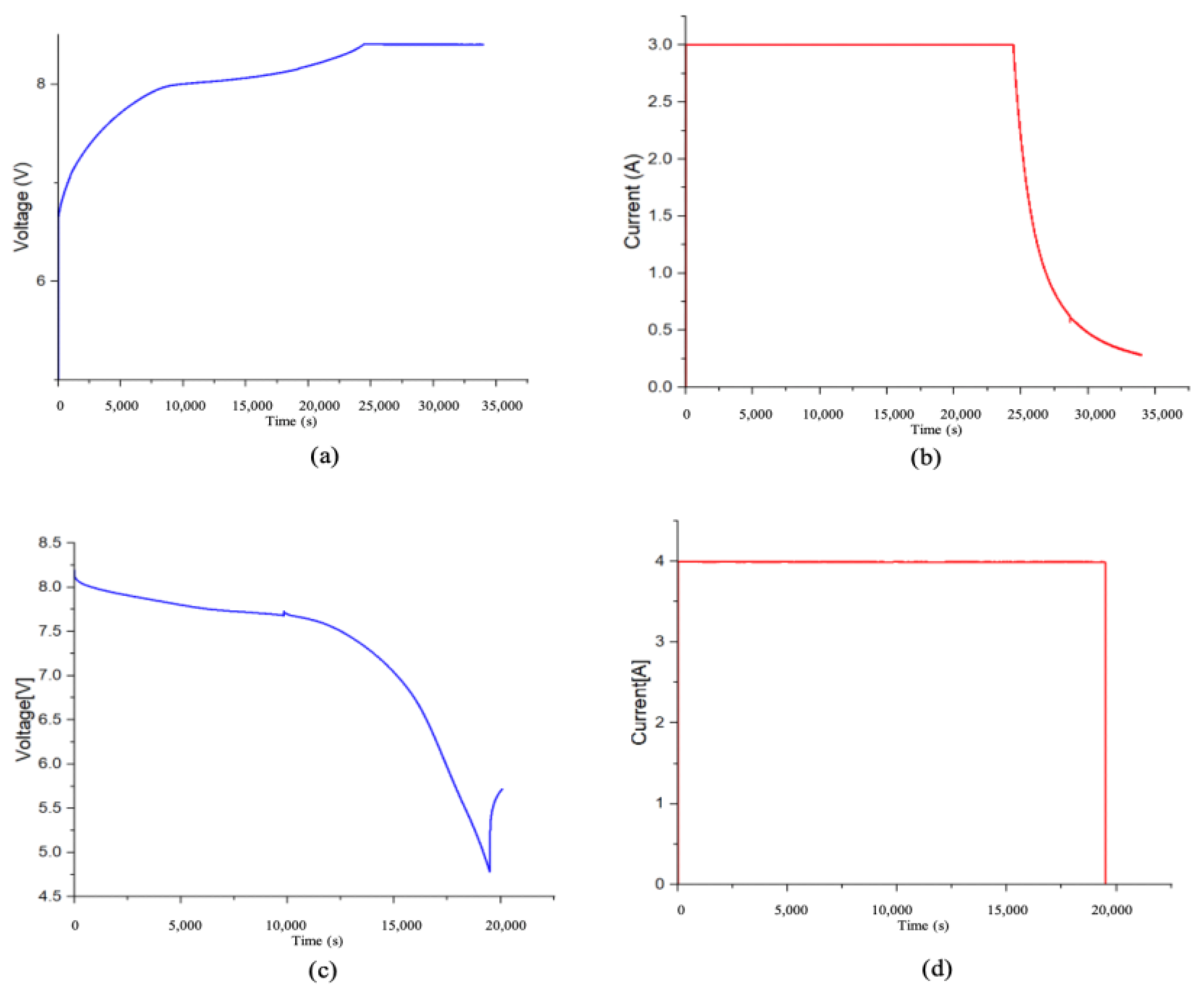
The charging and discharging current and voltage curves over time of the Nissan Leaf module exhibit the same pattern as those of the 18650 battery datasets. The only difference between the training dataset and the Nissan Leaf Gen 01 battery module lies in the capacity when comparing their performance. Therefore, normalization was performed using standard data for each battery type. This process brings both battery values to a scale between 0 and 1, making the model well-suited for predicting the remaining useful life (RUL) of Nissan Leaf battery modules. These methods ensure that predictions remain robust despite the constraints encountered during data collection. It is important to note that this approach does not consider the battery’s chemistry or physical structure. Figure 7 illustrates the charge and discharge curves plotted using the gathered data. The standard times can be calculated as follows:
where 2 Ah is the capacity and 1.5 A is the charging current for the 18650 battery.
where 24 kW is the capacity, 48 is the number of modules in a pack, 3 A is the charging current, and 8.4 V is the max voltage of a Nissan Leaf battery module.
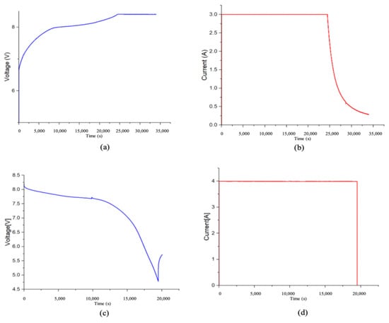
Figure 7.
Leaf Gen 01. (a) Charge voltage vs. time; (b) charge current vs. time; (c) discharge voltage vs. time; (d) discharge current vs. time.
2.3. Experiment
- Model Selection
We obtained the lithium-ion battery data from NASA’s Prognostic Center of Excellence (PCoE). For our model, we selected four battery cells designated as B0005, B0006, B0007, and B0018. These batteries underwent various operational profiles, including charging, discharging, and impedance testing, all conducted at room temperature. Charging was performed in constant current (CC) mode at 1.5 A until the battery voltage reached 4.2 V, followed by constant voltage (CV) mode until the charge current decreased to 20 mA. Discharging occurred at a constant current (CC) of 2 A until the battery voltages dropped to 2.7 V, 2.5 V, 2.2 V, and 2.5 V for batteries B0005, B0006, B0007, and B0018, respectively.
The experiments were terminated when the batteries met the end-of-life (EOL) criteria, defined as a 30% reduction in rated capacity (from 2 Ah to 1.4 Ah).
We used batteries B0005, B0006, and B0007, which had 167 cycles, to train the model, while battery B0018, with 132 cycles, was utilized for testing. Although the dataset from NASA includes several hundred cycles, the proposed model is capable of functioning effectively with cells that have a higher cycle count, especially since we normalized the target output using min–max normalization.
The DNN model was then trained using the encoded features from batteries B0005, B0006, and B0007, and tested with the encoded features of battery B0018 and CALCE lab data. The predicted results were compared among the DNN, Neural Network with memory features (NNwMF), Support Vector Machine (SVM), and Linear Regression (LR) models using RMSE% values. Under the NNwMF framework, we considered the DNN with PCA encoded memory features, DNN with memory features without encoding, DNN with memory features encoded using an autoencoder, and an LSTM model.
- B.
- Model Retraining
As the above-mentioned model is used to predict the remaining useful life (RUL) of Nissan Leaf batteries, maintaining the same test conditions as those in the training dataset can be challenging. Consequently, measuring certain parameters, such as temperature variation during the charging and discharging processes, becomes difficult. During the data collection phase, we focused solely on charging and discharging currents, voltage, and power over time, while neglecting temperature features. As a result, we had to retrain the most effective model obtained during our initial training phase using the new set of 12 input features, making it suitable for predicting the remaining useful life (RUL) of the Nissan Leaf Gen 01 battery modules.
3. Results and Discussion
- Results of Encoding Techniques
When implementing memory features, it is essential to compress the input features into lower dimensions without compromising the integrity of the original data, as this could negatively impact the model’s accuracy.
- PCA
PCA is one of the encoding techniques utilized in this study. The accuracy is evaluated by comparing the plot of the original data with the plot generated from the encoded and decoded data. The R-squared method was employed to assess the accuracy of the PCA, with an R-squared value of 100% indicating a perfect match between the graphs. Table 3 presents the accuracy of the PCA for different n values.
Table 3.
Accuracy of PCA.
- ii.
- Autoencoder
An autoencoder is a neural network model used as an encoding technique. Accuracy is measured using the RMSE (%) value. Table 4 displays the accuracy of the autoencoder for various values of n.
Table 4.
Accuracy of autoencoder.
- B.
- Results for Different ML Models
Initially, we developed three machine learning models: Linear Regression, Support Vector Machine (SVM), and a Deep Neural Network (DNN).
These models were trained using data from the B0005, B0006, and B0007 batteries, and predictions were made for the B0018 battery. The RMSE values were calculated to compare the models and identify the one with the highest accuracy.
Table 5 illustrates the accuracies of the three models. The DNN model was chosen due to its lowest validation loss, leading to further optimization of the model. Figure 8 shows the result for the selected DNN model before implementing memory features (MFs).
Table 5.
Accuracy of different ML models.
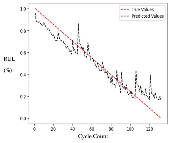
Figure 8.
Output of DNN without memory features.
- C.
- Performance Analysis of Neural Network Models with Memory Features
Multiple experiments were conducted with the incorporation of memory features, yielding promising results. The process was repeated for different n values, where n represents the number of previous cycles considered for predicting the RUL. Table 6 presents how the RMSE value varies across the DNN model with an autoencoder, the DNN model with PCA, the DNN model without PCA, and the LSTM model as the number of previous cycles increases.
Table 6.
Accuracy of different neural network models.
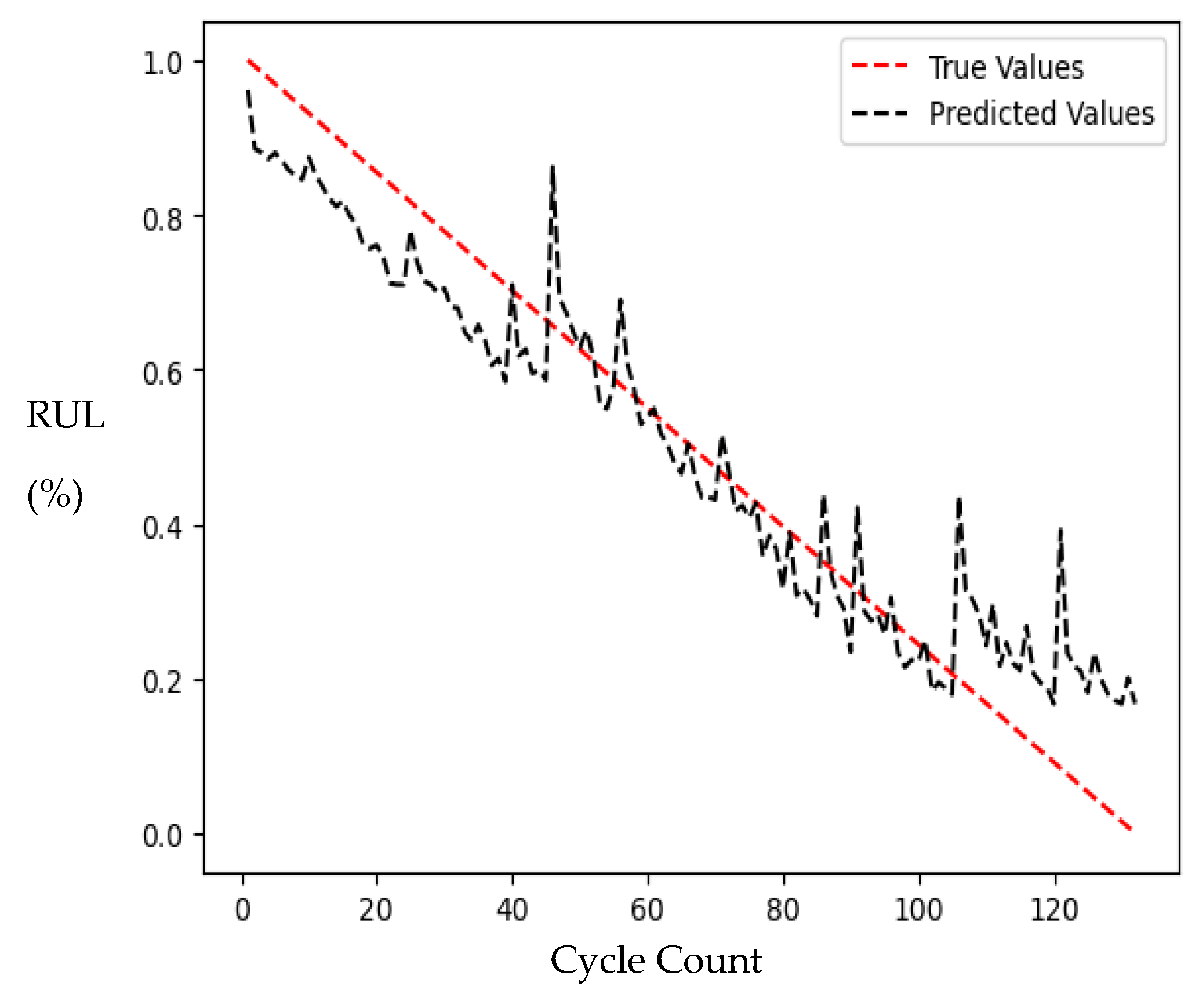
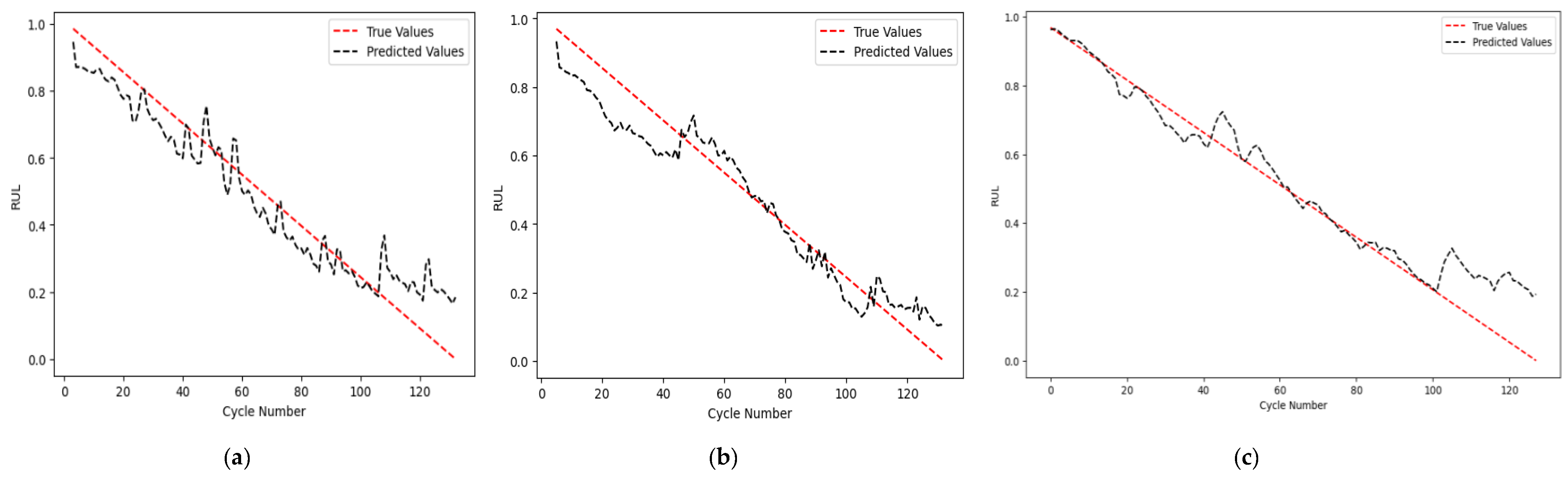
Figure 9 presents the optimal Predicted RUL compared to the True RUL for each NN model, where subfigure (a) shows the performance of the DNN with autoencoder for n = 2 with an RMSE value of 6. 21%, (b) illustrates the DNN with PCA for n = 4 with an RMSE value of 7.72%, and (c) shows the LSTM for n = 4 with an RMSE of 7.81%. Each model demonstrates its best accuracy at the corresponding n values.
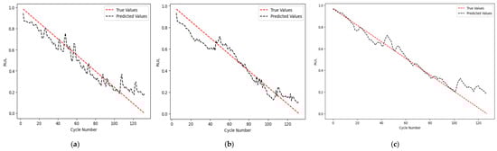
Figure 9.
Model outputs. (a) DNN with autoencoder for n = 2; (b) DNN with PCA for n = 4; (c) LSTM for n = 4.
- D.
- Nissan Leaf Battery Predictions compared to BMS reading
Since the DNN with an autoencoder demonstrated the highest accuracy, achieving the lowest RMSE value of 6.61% at n = 2, it was utilized for predicting the RUL of the recently retired Nissan Leaf battery module after retraining the model. The RMSE of the retrained model was 7.89%. The predicted values were compared against the BMS readings of the battery pack, assuming that the battery modules share the same RUL as the packs. Three battery modules (B1, B2, B3) were selected from different state of health (SOH) ranges. Each Nissan Leaf battery underwent complete charging and discharging processes several times: B1 completed five full cycles, while B2 and B3 completed four cycles each. As we incorporated memory features for n = 2, data from three consecutive cycles were required (including two prior cycles). For example, with B1, if the cycles are named C1, C2, C3, C4, and C5:
Set 1 considers the state of C3, using C2 and C1 as memory features.
Set 2 considers the state of C4, using C3 and C2 as memory features.
Set 3 considers the state of C5, using C4 and C3 as memory features.
Similarly, for B2 and B3, two tests were performed for each battery module, following the same logic.
Altogether, for B1, we performed three predictions, and for B2 and B3, we performed two predictions each. The results for each prediction using Deep Neural Network are presented in Table 7.
Table 7.
Nissan Leaf battery module prediction.
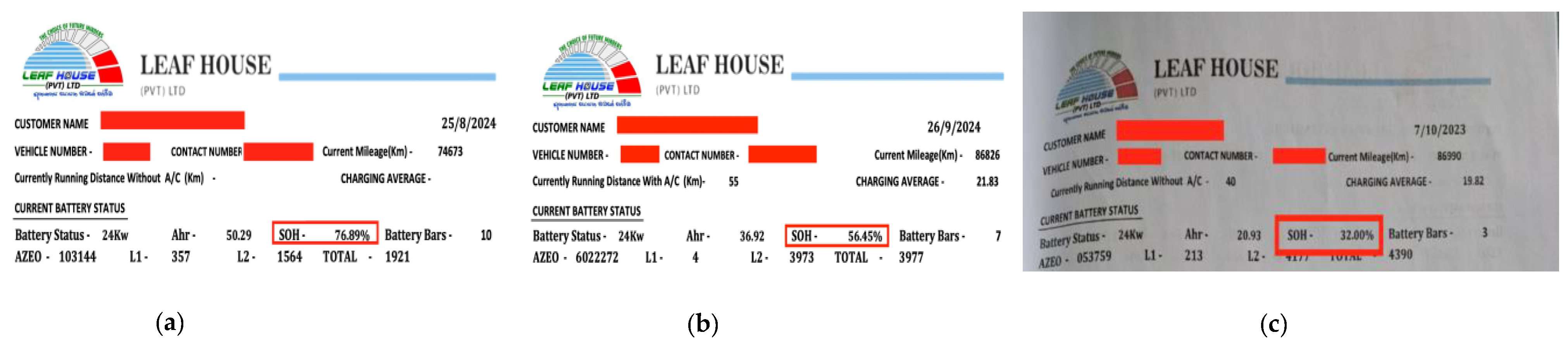
Figure 10 shows the remaining useful life (RUL) displayed by the integrated battery management system (BMS) of Nissan Leaf cars at the time of battery removal. This BMS estimates the RUL by tracking the history of the charging and discharging cycles. Sub figures (a), (b), and (c) show the readings for the B1, B2, and B3 batteries, respectively.
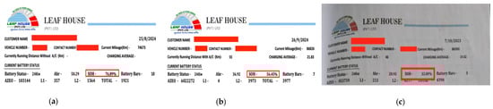
Figure 10.
BMS readings for battery. (a) B1; (b) B2; (c) B3. Red box indicates State of Health at removal.
4. Conclusions
This study presents a novel deep learning approach for predicting the remaining useful life (RUL) of lithium-ion battery (LIB) cells. The methodology involves a feature extraction process that reveals meaningful patterns from time series data, demonstrating the effectiveness of the model in improving RUL prediction accuracy in a normalized manner. Through experimentation, it was found that the Deep Neural Network (DNN) model with memory features (DNNwMF) combined with an autoencoder is optimal for this task, outperforming various machine learning techniques, including RNN (LSTM), SVM, and Linear Regression.
The optimized model achieved a Root Mean Squared Error (RMSE) of 6.61% during testing with the training dataset and demonstrated a prediction accuracy of 92.11% for the retrained model used to predict the RUL of Nissan Leaf battery modules. This predictive capability highlights its suitability for practical applications, including second-life uses for retired batteries. The proposed method’s robust performance over traditional models and its practical applicability make it a promising tool for enhancing battery management systems and extending the lifespan of lithium-ion batteries across diverse applications.
However, the current methodology has certain limitations. The time required to complete a full charge–discharge cycle is approximately two days, which poses a constraint for large-scale or real-time implementations. Additionally, the model has only been validated on Nissan Leaf Gen 1 battery modules, limiting its generalizability across different battery models and chemistries.
In real-world scenarios, this model can be integrated into advanced battery management systems (BMSs) to enable predictive maintenance, reduce unexpected battery failures, and support the design of energy-efficient charging and discharging strategies. It can also inform decisions in electric vehicle fleet management, grid storage optimization, and circular economy initiatives by accurately identifying end-of-life batteries suitable for secondary use. Furthermore, the methodological framework of combining memory features with autoencoders opens up avenues for future research in developing generalizable models across different battery chemistries and operational conditions.
Future work will focus on optimizing the model to function effectively with a reduced number of previous cycle data points (e.g., memory features with n = 1 or n = 2), which can significantly lower the data acquisition time and make the model more feasible for real-time applications. Additionally, efforts will be made to generalize the model across various Nissan Leaf battery modules and explore lightweight architectures suitable for edge deployment. Uncertainty quantification and safety-driven RUL models under extreme conditions will also be considered to ensure more reliable and interpretable outcomes.
Author Contributions
Conceptualization, S.M.W., D.M.P.A., S.A.D.S. and V.L.; methodology, S.M.W.; validation, D.M.P.A.; formal analysis, S.A.D.S.; resources, C.W.; data curation, S.M.W.; writing—original draft preparation, S.M.W.; writing—review and editing, S.A.D.S.; visualization, D.M.P.A.; supervision, V.L. and C.W.; funding acquisition, C.W. All authors have read and agreed to the published version of the manuscript.
Funding
This research received no external funding.
Data Availability Statement
The CALCE laboratory data used in this study are publicly available on the official CALCE Lab website at https://calce.umd.edu. The NASA dataset is accessible through the NASA open data portal at https://data.nasa.gov/organization/nasa. The Leaf battery datasets used and/or analyzed during the current study are available from the corresponding author upon reasonable request.
Acknowledgments
We thank NASA labs for providing the data used in this project. We also express our gratitude to Michael Pecht, founder and director of CALCE labs at the University of Maryland, for his valuable advice and for providing lab data. Additionally, we appreciate LEAF HOUSE (PVT) LTD for supplying the Nissan Leaf batteries essential for this work.
Conflicts of Interest
The authors declare no conflicts of interest.
Abbreviations
The following abbreviations are used in this manuscript:
| CALCE | Center for Advanced Life Cycle Engineering |
References
- Wickramaarachchi, S.M.; Suraweera, S.A.D.; Akalanka, D.M.P.; Logeeshan, V.; Wanigasekara, C. Accurate Prediction of Remaining Useful Life for Lithium-ion Battery Cells Using Deep Neural Networks. In Proceedings of the 2024 IEEE World AI IoT Congress (AIIoT), Seattle, WA, USA, 29–31 May 2024; pp. 562–568. [Google Scholar]
- Ellis, B.L.; Lee, K.-T.; Nazar, L.F. Positive electrode materials for Li-Ion and Li-Batteries. Chem. Mater. 2010, 22, 691–714. [Google Scholar] [CrossRef]
- Vermeer, W.; Mouli, G.R.C.; Bauer, P. A comprehensive review on the characteristics and modeling of Lithium-Ion battery aging. IEEE Trans. Transp. Electrification 2022, 8, 2205–2232. [Google Scholar] [CrossRef]
- Han, X.; Lu, L.; Zheng, Y.; Feng, X.; Li, Z.; Li, J.; Ouyang, M. A review on the key issues of the lithium ion battery degradation among the whole life cycle. eTransportation 2019, 1, 100005. [Google Scholar] [CrossRef]
- Tsiropoulos, I.; Tarvydas, D.; Natalia, L. Li-ion Batteries for Mobility and Stationary Storage Applications; EU Publications: Luxembourg, 2018. [Google Scholar]
- Wang, Z.; Liu, Y.; Wang, F.; Wang, H.; Su, M. Capacity and remaining useful life prediction for lithium-ion batteries based on sequence decomposition and a deep-learning network. J. Energy Storage 2023, 72, 108085. [Google Scholar] [CrossRef]
- Hasib, S.A.; Islam, S.; Chakrabortty, R.K.; Ryan, M.J.; Saha, D.K.; Ahamed, M.H.; Moyeen, S.I.; Das, S.K.; Ali, F.; Islam, R.; et al. A comprehensive review of available battery datasets, RUL prediction approaches, and advanced battery management. IEEE Access 2021, 9, 86166–86193. [Google Scholar] [CrossRef]
- Pang, X.; Huang, R.; Wen, J.; Shi, Y.; Jia, J.; Zeng, J. A lithium-ion battery RUL prediction method considering the capacity regeneration phenomenon. Energies 2019, 12, 2247. [Google Scholar] [CrossRef]
- Pan, C.; Huang, A.; He, Z.; Chang, L.; Sun, Y.; Zhao, S.; Wang, L. Prediction of remaining useful life for lithium-ion battery based on particle filter with residual resampling. Energy Sci. Eng. 2021, 9, 1115–1133. [Google Scholar] [CrossRef]
- Ren, L.; Li, Z.; Hong, S.; Zhao, S.; Wang, H.; Zhang, L. Remaining useful life prediction for Lithium-Ion Battery: A deep learning approach. IEEE Access 2018, 6, 50587–50598. [Google Scholar] [CrossRef]
- Zhang, Y.; Xiong, R.; He, H.; Pecht, M.G. Long Short-Term Memory Recurrent Neural Network for Remaining Useful Life Prediction of Lithium-Ion Batteries. IEEE Trans. Veh. Technol. 2018, 67, 5695–5705. [Google Scholar] [CrossRef]
- Liu, J.; Saxena, A.; Goebel, K.; Saha, B.; Wang, W. An Adaptive Recurrent Neural Network for Remaining Useful Life Prediction of Lithium-ion Batteries. In Proceedings of the Annual Conference of the PHM Society, Portland, OR, USA, 10–16 October 2010; Volume 2. [Google Scholar]
- Wen, J.; Yu, Y.; Chen, C. A Review on Lithium-Ion Batteries Safety Issues: Existing Problems and Possible Solutions. Mater. Express 2012, 2, 197–212. [Google Scholar] [CrossRef]
- Xu, X.; Chen, N. A state-space-based prognostics model for lithium-ion battery degradation. Reliab. Eng. Syst. Saf. 2017, 159, 47–57. [Google Scholar] [CrossRef]
- Zhang, Y.; Xiong, R.; He, H.; Pecht, M.G. Lithium-Ion Battery Remaining Useful Life Prediction With Box–Cox Transformation and Monte Carlo Simulation. IEEE Trans. Ind. Electron. 2019, 66, 1585–1597. [Google Scholar] [CrossRef]
- Nuhic, A.; Terzimehic, T.; Soczka-Guth, T.; Buchholz, M.; Dietmayer, K. Health diagnosis and remaining useful life prognostics of lithium-ion batteries using data-driven methods. J. Power Sources 2013, 239, 680–688. [Google Scholar] [CrossRef]
- Kandadi, T.; Shankarlingam, G. Drawbacks of LSTM Algorithm: A Case Study. 2025. Available online: https://ssrn.com/abstract=5080605 (accessed on 6 June 2025).
- Yeh, C.-N.; Rose, J.; Thaman, H.; Narasimhan, S.; Huang, W.-Y.; Sun, W.; Huang, W.; Zhang, Z.; Chueh, W.C. Lithium Plating on Graphite Electrodes in Lithium-Ion Batteries. In ECS Meeting Abstracts; The Electrochemical Society, Inc.: Pennington, NJ, USA, 2024; Volume MA2024-02, p. 532. [Google Scholar]
- Pranolo, A.; Setyaputri, F.U.; Paramarta, A.K.I.; Triono, A.P.P.; Fadhilla, A.F.; Akbari, A.K.G.; Utama, A.B.P.; Wibawa, A.P.; Uriu, W. Enhanced Multivariate Time Series Analysis Using LSTM: A Comparative Study of Min-Max and Z-Score Normalization Techniques. Ilk. J. Ilm. 2024, 16, 210–220. [Google Scholar] [CrossRef]
- Thorstensen, N.; Segonne, F.; Keriven, R. Normalization and preimage problem in gaussian kernel PCA. In Proceedings of the 2008 15th IEEE International Conference on Image Processing, San Diego, CA, USA, 12–15 October 2008; pp. 741–744. [Google Scholar]
- Guan, P.; Zhang, T.; Zhou, L. RUL Prediction of Rolling Bearings Based on Multi-Information Fusion and Autoencoder Modeling. Processes 2024, 12, 1831. [Google Scholar] [CrossRef]
- Gao, W.; Cao, Z.; Kurdkandi, N.V.; Fu, Y.; Mi, C. Evaluation of the second-life potential of the first-generation Nissan Leaf battery packs in energy storage systems. eTransportation 2024, 20, 100313. [Google Scholar] [CrossRef]
Disclaimer/Publisher’s Note: The statements, opinions and data contained in all publications are solely those of the individual author(s) and contributor(s) and not of MDPI and/or the editor(s). MDPI and/or the editor(s) disclaim responsibility for any injury to people or property resulting from any ideas, methods, instructions or products referred to in the content. |
© 2025 by the authors. Licensee MDPI, Basel, Switzerland. This article is an open access article distributed under the terms and conditions of the Creative Commons Attribution (CC BY) license (https://creativecommons.org/licenses/by/4.0/).