Second-Order Modified Nonstandard Explicit Euler and Explicit Runge–Kutta Methods for n-Dimensional Autonomous Differential Equations

Abstract

Nonstandard finite-difference (NSFD) methods, pioneered by R. E. Mickens, offer accurate and efficient solutions to various differential equation models in science and engineering. NSFD methods avoid numerical instabilities for large time steps, while numerically preserving important properties of exact solutions. However, most NSFD methods are only first-order accurate. This paper introduces two new classes of explicit second-order modified NSFD methods for solving n-dimensional autonomous dynamical systems. These explicit methods extend previous work by incorporating novel denominator functions to ensure both elementary stability and second-order accuracy. This paper also provides a detailed mathematical analysis and validates the methods through numerical simulations on various biological systems.

1. Introduction

Dynamical systems are important in many disciplines, including biology, economics, engineering, and chemistry. Because the majority of dynamical systems cannot be solved analytically, numerical methods are typically used to approximate their solutions. However, the stability properties of the corresponding numerical solutions are typically strongly dependent on the computational step size, particularly when standard numerical methods such as the explicit Euler and Runge–Kutta methods are used. R.E. Mickens [1] pioneered the use of nonstandard finite-difference (NSFD) methods to overcome this dependency while numerically preserving important properties of exact solutions. Since then, NSFD methods have been developed and applied to a wide range of scientific and engineering problems. Notably, NSFD methods have been constructed for numerically solving problems in ecology [2,3,4,5,6,7,8] and epidemiology [9,10,11,12,13,14,15,16,17,18,19,20,21,22], for solving biochemical systems [23,24], and general productive-destructive systems [25,26], to name a few. For a detailed review of various NSFD methods, we refer the reader to [27,28,29]. In particular, several classes of NSFD methods have been developed based on standard theta methods and standard two-stage explicit Runge–Kutta (ERK2) methods [18,30,31,32]. However, these methods, while preserving the local dynamical properties of solutions near equilibrium points, are only first-order accurate. There exist some higher-order nonstandard numerical methods, such as those presented in [23,25]; however, their elementary stability property has not yet been established analytically. In [14], the proposed class of NSFD methods is elementary stable but is second-order accurate only for a very specific choice of parameters. In [33], a second-order nonstandard method based on the Runge–Kutta methods is presented, but the proposed elementary stable nonstandard explicit Euler’s method is only of first-order accuracy. Recently, modified nonstandard theta and Runge–Kutta methods [34,35] that are not only elementary stable but also second-order accurate have been presented. But, those methods were only developed for one-dimensional autonomous dynamical systems.

This paper contributes to the field of NSFD methods by presenting two novel generalized versions of the NSFD explict Euler and NSFD explicit Runge–Kutta methods, which are not only elementary stable but also second-order accurate, with the order of accuracy of the underlying numerical method being improved in the case of the explicit Euler method. Here, previous theoretical results are extended, and new explicit second-order modified NSFD methods for solving n-dimensional autonomous dynamical systems are designed. The extensions are based on the use of novel denominator functions that account for both the elementary stability and the increased accuracy of the numerical methods. The modified NSFD methods are applied for solving a forest biomass model, an epidemiological model, and a predator–prey model. The numerical simulation results demonstrate the superior performance of the proposed new NSFD methods.

This paper is structured as follows. The new explicit second-order modified NSFD methods are constructed and analyzed in Section 2. Applications to two classical mathematical biology models are presented in Section 3 to numerically validate the theoretical results. In Section 4, some concluding remarks are made and future research directions are outlined.

2. Main Results

An n-dimensional autonomous differential equation can be written as

$${\overrightarrow{x}}^{\prime }(t)=\overrightarrow{f}(\overrightarrow{x});\overrightarrow{x}(t_0)={\overrightarrow{x}}_0,$$

(1)

where $\overrightarrow{x}$ represents the vector function ${[x_1(t),\dots ,x_n(t)]}^T$, $x_i:[t_0,T)\to \mathbb{R}$, $\overrightarrow{f}={[f_1,\dots ,f_n]}^T$$\in C^2({\mathbb{R}}^n;{\mathbb{R}}^n)$ is differentiable, ${\overrightarrow{x}}_0\in {\mathbb{R}}^n$. It is assumed that System (1) has a finite number of only hyperbolic equilibria. For NSFD methods in the case of systems with non-hyperbolic equilibria, see [36,37,38].

Definition 1.

Let ${\overrightarrow{x}}^{\ast }$ be an equilibrium of System (1), $J({\overrightarrow{x}}^{\ast })={\left({\displaystyle \frac{\partial f_i}{\partial x_j}}({\overrightarrow{x}}^{\ast })\right)}_{1\le i,j\le n}$ be the Jacobian of System (1) at ${\overrightarrow{x}}^{\ast }$, with $\sigma (J({\overrightarrow{x}}^{\ast }))$ denoting the spectrum of $J({\overrightarrow{x}}^{\ast })$. An equilibrium ${\overrightarrow{x}}^{\ast }$ of System (1) is called linearly stable if $Re(\lambda )<0$ for $\lambda \in \sigma (J({\overrightarrow{x}}^{\ast }))$, and linearly unstable if $Re(\lambda )>0$ for some $\lambda \in \sigma (J({\overrightarrow{x}}^{\ast }))$.

A general finite-difference method which approximates the solution of System (1) on the interval $[t_0,T]$ can be written as

$$D_{i,h}({\overrightarrow{x}}^k)=F_{i,h}(f_i;{\overrightarrow{x}}^k),k=0,\dots ,N_t,$$

(2)

where ${\left.D_{i,h}({\overrightarrow{x}}^k)\approx x_i^{\prime }\right|}_{t=t_k}$, $F_{i,h}(f_i;{\overrightarrow{x}}^k)\approx f_i(\overrightarrow{x})$, ${\overrightarrow{x}}^k\approx \overrightarrow{x}(t_k)$, $t_k=t_0+kh$, $k=0,\dots ,N_t$, $i=1,\dots ,n$, with mesh size $h>0$.

The modified NSFD numerical methods discussed in this paper satisfy the two main properties of NSFD methods, as formalized by Anguelov and Lubuma in [30] (see [32,39]), which are that the denominator function ${\phi }_i(h)$, $i=1,2,\dots ,n$, from the discretization of the derivative, i.e., $D_{i,h}({\overrightarrow{x}}^k)={\displaystyle \frac{x_i^{k+1}-x_i^k}{{\phi }_i(h)}}$, is a non-negative function of the form ${\phi }_i(h)=h+\mathcal{O}(h^2)$, and the right-hand side function is discretized using multiple steps, i.e., $F_{i,h}(\overrightarrow{f};{\overrightarrow{x}}^k)=g_i({\overrightarrow{x}}^k,{\overrightarrow{x}}^{k+1},h)$, where $g_i({\overrightarrow{x}}^k,{\overrightarrow{x}}^{k+1},h)$ is a multi-step approximation of the i component of the right-hand side of System (1).

Definition 2

([30,32,39]). A finite-difference method is elementary stable if, for any value of the step size h, its only fixed points ${\overrightarrow{x}}^{\ast }$ are the same as the equilibria of Equation (1) and the local stability properties of each ${\overrightarrow{x}}^{\ast }$ are the same for both the differential equation and the discrete method.

2.1. General Second-Order Modified Nonstandard Explicit Euler Method

The new second-order modified nonstandard explicit Euler method is given in the following theorem:

Theorem 1. 

Let $\overrightarrow{f}\in C^2({\mathbb{R}}^n;{\mathbb{R}}^n)$ and let ${\phi }_i:{\mathbb{R}}^{+}\times {\mathbb{R}}^n\to {\mathbb{R}}^{+}$, for $i=1,\dots ,n$, which satisfies the following conditions:

 (I)

$${\displaystyle {\phi }_i(h,\overrightarrow{x})=\left\{\begin{array}{cc}{\displaystyle h+\frac{⟨{\nabla }_x{f}_i(\overrightarrow{x}),\overrightarrow{f}(\overrightarrow{x})⟩}{f_i(\overrightarrow{x})}\frac{h^2}{2}+\mathcal{O}(h^3),}\hfill & f_i(\overrightarrow{x})\ne 0\hfill \\ {\displaystyle h,}\hfill & f_i(\overrightarrow{x})=0\hfill \end{array}\right.,}$$

for all $1\le i\le n$.

 (II)

${\displaystyle 0<{\phi }_i(h,\overrightarrow{x})<\frac{2|Re({\lambda }_i)|}{|{\lambda }_i{|}^2}}$, for all hyperbolic equilibria ${\overrightarrow{x}}^{\ast }$ of Equation (1) with $h>0$ and for all $\overrightarrow{x}\in {\mathbb{R}}^n$.

• Then, the modified nonstandard explicit Euler method

$${\displaystyle \frac{x_i^{k+1}-x_i^k}{{\phi }_i(h,{\overrightarrow{x}}^k)}}=f_i\left({\overrightarrow{x}}^k\right)$$

(3)

$i=1,\dots ,n$, for approximating the solution of Equation (1), is both second-order accurate and elementary stable.

Proof. 

The second-order accuracy of the modified nonstandard explicit Euler method (3) is proven using the Taylor series expansion about $t_k$, which yields

• If $f_i({\overrightarrow{x}}^k)\ne 0$, then

  $$\begin{array}{cc}\hfill & x_i(t_{k+1})-\left[x_i(t_k)+{\phi }_i(h,\overrightarrow{x}(t_k))f_i\left(\overrightarrow{x}(t_k)\right)\right]\hfill \\ \hfill & =\left[x_i(t_k)+h{x}_i^{\prime }(t_k)+{\displaystyle \frac{h^2}{2}}{x}^{″}(t_k)+\mathcal{O}(h^3)\right]-\left[x_i(t_k)+{\phi }_i(h,\overrightarrow{x}(t_k))f_i(\overrightarrow{x}(t_k))\right]\hfill \\ \hfill & =h{x}_i^{\prime }(t_k)+{\displaystyle \frac{h^2}{2}}{x}_i^{″}(t_k)-{\phi }_i(h,\overrightarrow{x}(t_k))f_i(\overrightarrow{x}(t_k))+\mathcal{O}(h^3)\hfill \\ \hfill & =h{f}_i(\overrightarrow{x}(t_k))+{\displaystyle \frac{h^2}{2}}⟨{\nabla }_x{f}_i(\overrightarrow{x}(t_k)),\overrightarrow{f}(\overrightarrow{x}(t_k))⟩-h{f}_i(\overrightarrow{x}(t_k))-{\displaystyle \frac{h^2}{2}}⟨{\nabla }_x{f}_i(\overrightarrow{x}(t_k)),\overrightarrow{f}(\overrightarrow{x}(t_k))⟩+\mathcal{O}(h^3)\hfill \\ \hfill & =\mathcal{O}(h^3).\hfill \end{array}$$
• If $f_i({\overrightarrow{x}}^k)=0$, then the numerical method (3) reduces to $x_i^{k+1}=x_i^k$, which represents an exact scheme for solving Equation (1) at $t=t_k$.

Therefore, the numerical method (3) is of second-order accuracy.

To prove the elementary stability of the NSFD method (3), we assume that System (1) has a finite number of only hyperbolic equilibria.

First, we need to show that the fixed points of Scheme (3) are equilbrium points to System (1) and vise versa. Suppose that ${\overrightarrow{x}}^{\ast }$ is a fixed point of Scheme (3). Then,

$$x_i^{\ast }=x_i^{\ast }+{\phi }_i(h,{\overrightarrow{x}}^{\ast })f_i\left({\overrightarrow{x}}^{\ast }\right),$$

for all $i=1,\dots ,n$, this clearly implies $f_i({\overrightarrow{x}}^{\ast })=0$, i.e., ${\overrightarrow{x}}^{\ast }$ is an equilibrium point to System (1). If ${\overrightarrow{x}}^{\ast }$ is an equilibrium point to System (1), then $f_i({\overrightarrow{x}}^{\ast })=0$, and we need to show that

$$x_i^{\ast }=x_i^{\ast }+{\phi }_i(h,{\overrightarrow{x}}^{\ast })f_i\left({\overrightarrow{x}}^{\ast }\right),$$

(4)

and Equation (4) clearly holds.

Next, let ${\overrightarrow{x}}^{\ast }$ be a hyperbolic equilibrium of System (1) and $J=J(x^{\ast })$ be the Jacobian matrix evaluated at ${\overrightarrow{x}}^{\ast }$ with eigenvalues ${\lambda }_1,{\lambda }_2,\dots ,{\lambda }_n$. The corresponding linear system can then be given as follows:

$${\overrightarrow{x}}^{\prime }=J\overrightarrow{x}.$$

(5)

If $\mathsf{\Lambda }$ is a Jordan form of J, then $J=S^{-1}\mathsf{\Lambda }S$, where S is a non-singular complex $n\times n$ matrix. In general, $\mathsf{\Lambda }$ has the following bi-diagonal form:

$$\left(\begin{array}{cc}{\lambda }_1& {\alpha }_1\\ & {\lambda }_2& {\alpha }_2\\ & & \ddots & \ddots \\ & & & {\lambda }_{n-1}& {\alpha }_{n-1}\\ & & & & {\lambda }_n\end{array}\right),$$

where ${\lambda }_i\in \sigma (J)$, $i=1,2,\dots n$, and ${\alpha }_i=\{0,1\}$. Therefore, the linear system can be written as ${\overrightarrow{x}}^{\prime }=S^{-1}\mathsf{\Lambda }S\overrightarrow{x}$, and the change of variables $\overrightarrow{y}=S\overrightarrow{x}$ yields the following new system:

$${\overrightarrow{y}}^{\prime }=\mathsf{\Lambda }\overrightarrow{y}.$$

(6)

Applying the numerical method (3) on the above system results in the following:

$$\left[\begin{array}{c}{\displaystyle \frac{y_1^{k+1}-y_1^k}{{\phi }_1(h,{\overrightarrow{y}}^k)}}\\ {\displaystyle \frac{y_2^{k+1}-y_2^k}{{\phi }_2(h,{\overrightarrow{y}}^k)}}\\ ⋮\\ {\displaystyle \frac{y_n^{k+1}-y_n^k}{{\phi }_n(h,{\overrightarrow{y}}^k)}}\end{array}\right]=\mathsf{\Lambda }\left[\begin{array}{c}{\displaystyle y_1^k}\\ {\displaystyle y_2^k}\\ ⋮\\ {\displaystyle y_n^k}\end{array}\right]$$

(7)

and, equivalently, the following vector formulation:

$${\overrightarrow{y}}^{k+1}=(I+V\mathsf{\Lambda }){\overrightarrow{y}}^k,$$

(8)

where V is the diagonal matrix:

$$V=\left(\begin{array}{cc}{\phi }_1(h,{\overrightarrow{y}}^k)& \\ & {\phi }_2(h,{\overrightarrow{y}}^k)& & \\ & & \ddots & \\ & & & {\phi }_{n-1}(h,{\overrightarrow{y}}^k)& \\ & & & & {\phi }_n(h,{\overrightarrow{y}}^k)\end{array}\right).$$

Note that the matrix $(I+V\mathsf{\Lambda })$ is upper triangular and its eigenvalues are given by ${\mu }_i(h,{\overrightarrow{y}}^k)=1+{\lambda }_i{\phi }_i(h,{\overrightarrow{y}}^k)$, where ${\lambda }_i\in \sigma (J)$, $i=1,2,\dots ,n$. Observe that ${\overrightarrow{x}}^{\ast }$ being a stable fixed point of System (8) is equivalent to

$$\left|1+{\lambda }_i{\phi }_i(h,{\overrightarrow{y}}^k)\right|<1,$$

(9)

and therefore

$${|1+{\phi }_i(h,{\overrightarrow{y}}^k)Re({\lambda }_i)+{\phi }_i(h,{\overrightarrow{y}}^k)Im({\lambda }_i)|}^2<1.$$

From here, since ${\phi }_i(h,{\overrightarrow{y}}^k)>0$, a straightforward algebraic manipulation shows that Inequality (9) is equivalent to

$${\phi }_i(h,{\overrightarrow{y}}^k)<{\displaystyle \frac{-2Re({\lambda }_i)}{{\left|{\lambda }_i\right|}^2}}.$$

(10)

Note that Condition (II) implies

$$0<{\phi }_i(h,{\overrightarrow{y}}^k)<{\displaystyle \frac{2|Re({\lambda }_i)|}{{\left|{\lambda }_i\right|}^2}}.$$

If ${\overrightarrow{x}}^{\ast }$ is a locally stable equilibrium, then $|Re({\lambda }_i)|=-Re({\lambda }_i)$. Thus, from the above inequality, it can be seen that Inequality (10) holds. Hence, ${\overrightarrow{x}}^{\ast }$ is a stable fixed point. On the other hand, if ${\overrightarrow{x}}^{\ast }$ is an unstable equilibrium, then there is $j_0\in \left\{1,\dots ,n\right\}$, such that $Re({\lambda }_{j_0})>0$. This implies

$${\phi }_{j_0}(h,{\overrightarrow{y}}^k)>0>{\displaystyle \frac{-2Re({\lambda }_{j_0})}{{\left|{\lambda }_{j_0}\right|}^2}},$$

since ${\phi }_{j_0}(h,{\overrightarrow{y}}^k)>0$. Therefore, Inequality (10) is strictly not satisfied when ${\overrightarrow{x}}^{\ast }$ is an unstable equilibrium. As a result, ${\overrightarrow{x}}^{\ast }$ is an unstable fixed point. Therefore, the numerical scheme (3) is elementary stable. □

Lemma 1. 

If $f_i(\overrightarrow{x})\ne 0$, ${\varphi }_{i_1}:{\mathbb{R}}_{+}\to {\mathbb{R}}_{+}$ and ${\varphi }_{i_2}:\mathbb{R}\to {\mathbb{R}}_{+}$ satisfy the following conditions:

 (a)

$0<{\varphi }_{i_1}(h)<1$, for all $h>0$, and ${\varphi }_{i_1}(h)=h-{\displaystyle \frac{h^2}{2}}+\mathcal{O}(h^3).$

 (b)

$0<{\varphi }_{i_2}(h)<M$, for all $h\in \mathbb{R}$ and some $M>0$, and ${\varphi }_{i_2}(h)=1+h+\mathcal{O}(h^3).$

• Then, the functions

$${\phi }_i(h,\overrightarrow{x})={\displaystyle \frac{{\varphi }_{i_1}(\alpha h)}{\alpha }}{\varphi }_{i_2}\left({\displaystyle \frac{\alpha -q_i(\overrightarrow{x})}{2}}h\right),i=1,\dots ,n,$$

with $\alpha >{\displaystyle \frac{M}{2}}{max}_{\mathsf{\Omega }}{\displaystyle \frac{{\left|\lambda \right|}^2}{|Re(\lambda )|}}$, where $\mathsf{\Omega }={\bigcup }_{{\overrightarrow{x}}^{\ast }\in \mathsf{\Gamma }}\sigma (J({\overrightarrow{x}}^{\ast }))$ and Γ denotes the set of all equilibria of System (1) and $q_i(\overrightarrow{x})=-{\displaystyle \frac{⟨{\nabla }_x{f}_i(\overrightarrow{x}),\overrightarrow{f}(\overrightarrow{x})⟩}{f_i(\overrightarrow{x})}}$, satisfy the conditions $(I)$ and $(II)$ of Theorem (1).

Proof. 

Notice that

$$\begin{array}{cc}\hfill {\displaystyle \frac{{\varphi }_{i_1}(\alpha h)}{\alpha }}& =h-{\displaystyle \frac{\alpha h^2}{2}}+\mathcal{O}(h^3),\mathrm{and}\hfill \\ \hfill {\varphi }_{i_2}\left({\displaystyle \frac{\alpha -q_i(\overrightarrow{x})}{2}}h\right)& =1+{\displaystyle \frac{\alpha -q_i(\overrightarrow{x})}{2}}h+\mathcal{O}(h^3).\hfill \end{array}$$

Therefore,

$${\phi }_i(h,\overrightarrow{x})=h+{\displaystyle \frac{⟨{\nabla }_x{f}_i(\overrightarrow{x}),\overrightarrow{f}(\overrightarrow{x})⟩}{f_i(\overrightarrow{x})}}{\displaystyle \frac{h^2}{2}}+\mathcal{O}(h^3),$$

which proves Condition (I). Next, since $0<{\varphi }_{i_1}(h)<1$ and $0<{\varphi }_{i_2}(h)<M$, then one can easily see that

$$0<{\displaystyle \frac{{\varphi }_{i_1}(\alpha h)}{\alpha }}{\varphi }_{i_2}\left({\displaystyle \frac{\alpha -q_i(\overrightarrow{x})}{2}}h\right)<{\displaystyle \frac{M}{\alpha }}<{\displaystyle \frac{2\left|Re({\lambda }_i)\right|}{{\left|{\lambda }_i\right|}^2}},$$

Therefore, Condition (II) is also satisfied. □

Remark 1. 

There exists a variety of functions ${\varphi }_{i_1}$ and ${\varphi }_{i_2}$ that satisfy the conditions of Lemma 1. One such set of functions is ${\varphi }_{i_1}(h)=1-e^{-h}$ and ${\varphi }_{i_2}(h)=1+tanh(h)$, which can be used to construct the denominator functions ${\phi }_i(h,\overrightarrow{x})$ in Theorem 1.

Remark 2. 

The modified nonstandard implicit one-stage theta method

$${\displaystyle \frac{x_i^{k+1}-x_i^k}{{\phi }_i(h,{\overrightarrow{x}}^k)}}=f_i\left(\theta {\overrightarrow{x}}^{k+1}+(1-\theta ){\overrightarrow{x}}^k\right)$$

(11)

and the modified nonstandard implicit two-stage theta method

$${\displaystyle \frac{x_i^{k+1}-x_i^k}{{\phi }_i(h,{\overrightarrow{x}}^k)}}=\theta f_i({\overrightarrow{x}}^{k+1})+(1-\theta )f_i({\overrightarrow{x}}^k),$$

(12)

$i=1,\dots ,n$, where $\theta \in (0,1]$, for approximating the solution of Equation (1), are also both second-order accurate and elementary stable. Here, $\overrightarrow{f}\in C^2({\mathbb{R}}^n;{\mathbb{R}}^n)$ and ${\phi }_i:{\mathbb{R}}^{+}\times {\mathbb{R}}^n\to {\mathbb{R}}^{+}$, for $i=1,\dots ,n$, satisfies the following conditions:

 (I)

$${\displaystyle {\phi }_i(h,\overrightarrow{x})=\left\{\begin{array}{cc}{\displaystyle h+(1-2\theta )\frac{⟨{\nabla }_x{f}_i(\overrightarrow{x}),\overrightarrow{f}(\overrightarrow{x})⟩}{f_i(\overrightarrow{x})}\frac{h^2}{2}+\mathcal{O}(h^3),}\hfill & f_i(\overrightarrow{x})\ne 0\hfill \\ {\displaystyle h,}\hfill & f_i(\overrightarrow{x})=0\hfill \end{array}\right.,}$$

for all $1\le i\le n$.

 (II)

${\displaystyle 0<{\phi }_i(h,\overrightarrow{x})<\frac{2|Re({\lambda }_i)|}{|2\theta -1|{\left|{\lambda }_i\right|}^2}}$, $0<\theta \le 1$, $\theta \ne {\displaystyle \frac{1}{2}}$, for all hyperbolic equilibria ${\overrightarrow{x}}^{\ast }$ of Equation (1) with $h>0$ and for all $\overrightarrow{x}\in {\mathbb{R}}^n$,

2.2. General Second-Order Modified Nonstandard ERK2 Method

The following result holds for the new modified nonstandard two-stage ERK2 method:

Theorem 2. 

Let $\overrightarrow{f}=[f_1,\dots ,f_n]\in C^2({\mathbb{R}}^n;{\mathbb{R}}^n)$ and let $\phi :{\mathbb{R}}^{+}\to {\mathbb{R}}^{+}$ satisfy the following conditions:

 (I)

${\displaystyle \phi (h)=h+\mathcal{O}(h^3)}$,

 (II)

${\displaystyle 0<\phi (h)<\frac{1}{q}}$, for all $\lambda \in \mathsf{\Omega }$, where $q>{max}_{\mathsf{\Omega }}{\displaystyle \frac{{\left|\lambda \right|}^2}{2|Re(\lambda )|}}$, $\mathsf{\Omega }={\bigcup }_{{\overrightarrow{x}}^{\ast }\in \mathsf{\Gamma }}\sigma (J({\overrightarrow{x}}^{\ast }))$ and Γ denotes the set of all hyperbolic equilibria ${\overrightarrow{x}}^{\ast }$ of System (1).

• Then, the modified nonstandard two-stage ERK2 method for approximating the solution of Equation (1)

$$x_i^{k+1}=x_i^k+\phi (h)\left\{(1-\omega )f_i({\overrightarrow{x}}^k)+\omega f_i\left({\overrightarrow{x}}^k+{\displaystyle \frac{1}{2\omega }}\overrightarrow{f}({\overrightarrow{x}}^k)\phi (h)\right)\right\},0<\omega \le 1,$$

(13)

$i=1,\dots ,n$, is of second-order accuracy and preserves the local stability property of each ${\overrightarrow{x}}^{\ast }$, provided the method does not introduce additional fixed points other than those of Equation (1). Furthermore, when Equation (1) is conservative, then Method (13) is also conservative.

Proof. 

The second-order accuracy of the modified nonstandard two-stage ERK2 method (13) is proven using the Taylor series expansion about $t_k$, which yields

$$\begin{array}{cc}\hfill & x_i(t_{k+1})-\left[x_i(t_k)+\phi (h)\left\{(1-\omega )f_i(\overrightarrow{x}(t_k))+ \omega f_i\left(\overrightarrow{x}(t_k)+{\displaystyle \frac{1}{2\omega }}\overrightarrow{f}(\overrightarrow{x}(t_k))\phi (h)\right)\right\}\right]\hfill \\ \hfill & =\left[x_i(t_k)+h{x}_i^{\prime }(t_k)+{\displaystyle \frac{h^2}{2}}{x}_i^{″}(t_k)+\mathcal{O}(h^3)\right]-[x_i(t_k)+\phi (h)\{(1-\omega )f_i(\overrightarrow{x}(t_k))\hfill \\ \hfill & +\omega \left(f_i(\overrightarrow{x}(t_k))+{\displaystyle \frac{1}{2\omega }}\sum _{j=1}^n\phi (h)f_i(\overrightarrow{x}(t_k)){\displaystyle \frac{\partial f_i}{\partial x_j}}(\overrightarrow{x}(t_k))+\mathcal{O}(h^2)\right)\left\}\right]\hfill \\ \hfill & =x_i(t_k)+h{f}_i({\overrightarrow{x}}_{t_k})+{\displaystyle \frac{h^2}{2}}\sum _{j=1}^n{\displaystyle \frac{\partial f_i}{\partial x_j}}(\overrightarrow{x}(t_k))f_i(\overrightarrow{x}(t_k))-[x_i(t_k)+\phi (h)\{(1-\omega )f_i(\overrightarrow{x}(t_k))\hfill \\ \hfill & +\omega \left(f_i(\overrightarrow{x}(t_k))+{\displaystyle \frac{1}{2\omega }}\phi (h)\sum _{j=1}^n{f}_i(\overrightarrow{x}(t_k)){\displaystyle \frac{\partial f_i}{\partial x_j}}(\overrightarrow{x}(t_k))+\mathcal{O}(h^3)\right)\left\}\right]\hfill \\ \hfill & =(h-\phi (h))f_i(\overrightarrow{x}(t_k))+\left({\displaystyle \frac{h^2}{2}}-{\displaystyle \frac{{\phi }^2(h)}{2}}\right)\sum _{j=1}^n{\displaystyle \frac{\partial f_i}{\partial x_j}}(\overrightarrow{x}(t_k))f_i(\overrightarrow{x}(t_k))+\mathcal{O}(h^3)=\mathcal{O}(h^3),\hfill \end{array}$$

which implies the second-order accuracy of the numerical method (13).

To prove the elementary stability of the NSFD method (13), we assume that System (1) has a finite number of only hyperbolic equilibria. Let ${\overrightarrow{x}}^{\ast }$ be an hyperbolic equilibrium of System (1) and J be the Jacobian matrix evaluated at ${\overrightarrow{x}}^{\ast }$ with eigenvalues ${\lambda }_1,{\lambda }_2,\dots ,{\lambda }_n$. Let $\mathsf{\Lambda }$ be a Jordan form of J, given as follows:

$$\left(\begin{array}{cc}{\lambda }_1& {\alpha }_1\\ & {\lambda }_2& {\alpha }_2\\ & & \ddots & \ddots \\ & & & {\lambda }_{n-1}& {\alpha }_{n-1}\\ & & & & {\lambda }_n\end{array}\right)$$

where ${\lambda }_i\in \sigma (J)$, $i=1,2,\dots n$, and ${\alpha }_i=\{0,1\}$. Then, we have $J=S^{-1}\mathsf{\Lambda }S$. Using a similar argument as in the proof of Theorem 1, the numerical method (13) can be applied to

$${\overrightarrow{y}}^{\prime }=\mathsf{\Lambda }\overrightarrow{y},$$

(14)

where $\overrightarrow{y}=S\overrightarrow{x}$. This yields

$${\overrightarrow{y}}^{k+1}={\overrightarrow{y}}^k+\phi (h)\left\{(1-\omega )\mathsf{\Lambda }{\overrightarrow{y}}^k+\omega \mathsf{\Lambda }\left({\overrightarrow{y}}^k+{\displaystyle \frac{1}{2\omega }}\mathsf{\Lambda }{\overrightarrow{y}}^k\phi (h)\right)\right\},$$

which results in

$$\begin{array}{cc}\hfill {\overrightarrow{y}}^{k+1}& =\left[I+\phi (h)(1-\omega )\mathsf{\Lambda }+\omega \phi (h)\mathsf{\Lambda }\left(1+{\displaystyle \frac{1}{2\omega }}\phi (h)\mathsf{\Lambda }\right)\right]{\overrightarrow{y}}^k\hfill \\ \hfill & =\left[I+\phi (h)(1-\omega )\mathsf{\Lambda }+\omega \phi (h)\mathsf{\Lambda }+{\displaystyle \frac{1}{2}}{\phi }^2(h){\mathsf{\Lambda }}^2\right]{\overrightarrow{y}}^k\hfill \\ \hfill & =\left[I+\phi (h)\mathsf{\Lambda }+{\displaystyle \frac{1}{2}}{\phi }^2(h){\mathsf{\Lambda }}^2\right]{\overrightarrow{y}}^k.\hfill \end{array}$$

The eigenvalues of $I+\phi (h)\mathsf{\Lambda }+{\displaystyle \frac{1}{2}}{\phi }^2(h){\mathsf{\Lambda }}^2$ are given as

$${\mu }_i(h)=1+\phi (h){\lambda }_i+{\displaystyle \frac{1}{2}}{\lambda }_i^2{\phi }^2(h).$$

Therefore, showing that ${\overrightarrow{x}}^{\ast }$ is a stable equilibrium is equivalent to showing that $|{\mu }_i(h)|<1$ for all $i=1,\dots ,n$, i.e.,

$$|1+\phi (h){\lambda }_i+{\displaystyle \frac{1}{2}}{\lambda }_i^2{\phi }^2(h)|<1.$$

(15)

Inequality (15) corresponds to

$$\begin{array}{cc}& {\left(1+\phi (h)\mathrm{Re}({\lambda }_i)+{\displaystyle \frac{{\phi }^2(h)}{2}}\left\{{\left[\mathrm{Re}({\lambda }_i)\right]}^2-{\left[\mathrm{Im}({\lambda }_i)\right]}^2\right\}\right)}^2\hfill \\ \hfill +& {\phi }^2(h){(\mathrm{Im}({\lambda }_i))}^2{\left(1+\mathrm{Re}({\lambda }_i)\phi (h)\right)}^2<1,\hfill \end{array}$$

which is equivalent to

$${\displaystyle \frac{1}{4}}{\left|{\lambda }_i\right|}^4{\phi }^3(h)+Re({\lambda }_i){\left|{\lambda }_i\right|}^2{\phi }^2(h)+2{\left|{\lambda }_i\right|}^2\phi (h)+2Re({\lambda }_i)<0.$$

Denote $r_i(t)={\displaystyle \frac{1}{4}}{\left|{\lambda }_i\right|}^4{t}^3+Re({\lambda }_i){\left|{\lambda }_i\right|}^2{t}^2+2{\left|{\lambda }_i\right|}^{2}t+2Re({\lambda }_i)$. Thus, Inequality (15) is equivalent to $r_i(\phi (h))<0$ for each ${\lambda }_i$, where $i=1,2,\dots ,n$. Similarly, to show that ${\overrightarrow{x}}^{\ast }$ is an unstable equilibrium point is equivalent to showing that there exists an i, such that $r_i(\phi (h))>0$. The rest of the proof follows from [32].

Finally, the conservative property of the modified nonstandard two-stage ERK2 method (13) is proven. For this purpose, we assume that Equation (1) is conservative. First, observe that the denominator function $\phi (h)$ is independent of x and is thus the same for each component $i=1,\dots ,n$, of the numerical method. Next, summing over all $i=1,\dots ,n$ yields the following:

$$\begin{array}{cc}\hfill \sum _{i=1}^n{x}_i^{k+1}& =\sum _{i=1}^n{x}_i^k+\phi (h)\left\{(1-\omega )\sum _{i=1}^n{f}_i({\overrightarrow{x}}^k)+\omega \sum _{i=1}^n{f}_i\left({\overrightarrow{x}}^k+{\displaystyle \frac{1}{2\omega }}\overrightarrow{f}({\overrightarrow{x}}^k)\phi (h)\right)\right\}\hfill \end{array}$$

and, therefore,

$$\sum _{i=1}^n{x}_i^{k+1}=\sum _{i=1}^n{x}_i^k,$$

since ${\sum }_{i=1}^n{f}_i({\overrightarrow{x}}^k)={\sum }_{i=1}^n{f}_i\left({\overrightarrow{x}}^k+{\displaystyle \frac{1}{2\omega }}\overrightarrow{f}({\overrightarrow{x}}^k)\overrightarrow{\phi }(h)\right)=0$. □

Remark 3. 

All equilibria of System (1) are also fixed points of Method (13), since $f_i({\overrightarrow{x}}^{\ast })=0$ implies that

$$(1-\omega )f_i({\overrightarrow{x}}^{\ast })+\omega f_i\left({\overrightarrow{x}}^{\ast }+{\displaystyle \frac{1}{2\omega }}\overrightarrow{f}({\overrightarrow{x}}^{\ast })\phi (h)\right)=(1-\omega )f_i({\overrightarrow{x}}^{\ast })+\omega f_i({\overrightarrow{x}}^{\ast })=f_i({\overrightarrow{x}}^{\ast })=0$$

for $i=1,\dots ,n$ and ${\overrightarrow{x}}^{\ast }\in {\mathbb{R}}^n$; however, the vice versa is not necessarily always true. When all fixed points of Method (13) are also the equilibria of System (1), then Method (13) is elementary stable.

Remark 4. 

There exists a variety of functions $\phi (h)$ which satisfy the conditions of above Theorem 2, ensuring a second-order accurate and elementary stable method (13). One such denominator function is $\phi (h)={\displaystyle \frac{tanh(qh)}{q}}$, where $q>{max}_{\mathsf{\Omega }}{\displaystyle \frac{{\left|\lambda \right|}^2}{2|Re(\lambda )|}}$.

Remark 5. 

When analytical computations of the steady states and spectra of the Jacobian matrix for System (1) are difficult, numerical computations can be performed using any standard root-finding algorithms and power methods. Because those computations need to be carried out only once, at the beginning of the numerical implementation, they do not considerably increase the overall computational cost of the NSFD methods.

3. Numerical Simulations

In this section, the performance of the proposed new explicit second-order modified NSFD methods is illustrated. The modified NSFD explicit Euler (modified NSFD EE) method (12) and the modified nonstandard two-stage ERK2 method (13), with $\omega =1/2$, are chosen. Furthermore, the two-stage modified nonstandard ERK2 method (13) with $\omega =1/2$ is henceforth referred to as the modified NSFD ERK2 method. The modified NSFD methods are compared to other standard and nonstandard finite-difference methods for solving three specific biological systems.

For the numerical test cases, we consider a class of linear and nonlinear autonomous ODE systems. The linear system has an exact solution that enables us to compare the accuracy and performance of our proposed methods with other NSFD and non-NSFD methods. The nonlinear systems are used to demonstrate the performance of our proposed methods on general classes of autonomous ODEs.

In Test Case 1, we consider the following forest biomass model, presented in [40]:

$$\begin{array}{cc}\hfill x^{\prime }(t)& =-x(t)+3y(t)\hfill \\ \hfill y^{\prime }(t)& =-3y(t)+5z(t)\hfill \\ \hfill z^{\prime }(t)& =-5z(t),\hfill \end{array}$$

(16)

where $x(t)$ represents the biomass decayed into humus, $y(t)$ the biomass of dead trees, and $z(t)$ the biomass of living trees. The initial data are $x(0)=0$, $y(0)=0$, and $z(0)=z_0$, which assumes that there are no dead trees and no humus at $t=0$. The exact solution of the above system is given by

$$\begin{array}{cc}\hfill x(t)& ={\displaystyle \frac{15}{8}}(e^{-t}-2e^{-3t}+e^{-5t})z_0\hfill \\ \hfill y(t)& ={\displaystyle \frac{5}{2}}(e^{-3t}-e^{-5t})z_0\hfill \\ \hfill z(t)& =e^{-5t}{z}_0\hfill \end{array}$$

(17)

We compare our modified NSFD EE and modified NSFD ERK2 methods with the NSFD EE and NSFD ERK2 methods [32], the NSFD $\theta =\widehat{\theta }={\displaystyle \frac{1}{2}}$ and NSFD $\theta =0,\widehat{\theta }=1$ methods [10,14], the NSFD separate method ([40], Equation (23)), and the explicit Runge–Kutta methods of order four (RK4) [41], applied to Model (16). Figure 1a shows that all methods are working quite well for small values of the time step, particularly for $h=0.1$. It is also evident from Figure 1b, which shows the absolute error of all the methods, that the first-order methods have larger errors as compared to the second- and fourth-order methods. Figure 1c shows a comparison of the numerical methods for solving Model (16) using a large step size $h=0.569$, where we see that RK4 becomes unstable while the other nonstandard methods are converging to the solution even for large values of h. Finally, Figure 1d shows the order plots of all the numerical methods. A comparison of the $l^{\infty }$ errors at the final time $T=10$ and convergence rates for the numerical solution obtained with various NSFD methods is presented in Table 1. We define the $l^{\infty }$ error as

$$E(h)=\parallel x^h{-x\parallel }_{\infty },$$

where

$${\parallel y\parallel }_{\infty }=\underset{k=0,\dots ,N_t}{max}\left|y_k\right|$$

represents the discrete $l^{\infty }$ norm of the vector y, and x represents the exact solution of Equation (1). The errors are calculated by using the exact solution given in Equation (17). We observe from Table 1 that the solutions obtained using the modified NSFD EE and modified NSFD ERK2 methods converge to the exact solution with rate 2, which also validates our theoretical results and the observations made in Figure 1.

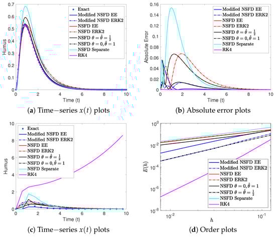
Figure 1. Test Case 1: Comparison of the modified NSFD EE and modified NSFD ERK2 methods to the NSFD EE, NSFD ERK2, NSFD $\theta =\widehat{\theta }={\displaystyle \frac{1}{2}}$, NSFD $\theta =0,\widehat{\theta }=1$, NSFD separate, and RK4 methods, applied to Model (16), using step size $h=0.1$ (a,b) and stepsize $h=0.569$ (c). The order plots for all eight methods are shown in (d). For illustration purposes, only plots of the biomass that has decayed into humus are shown.

Table 1. Test Case 1: Discrete $l^{\infty }$ error (top) and the rates of convergence (bottom) of the new modified NSFD EE and NSFD ERK2 methods, and the NSFD EE, NSFD ERK2, NSFD $\theta =\widehat{\theta }={\displaystyle \frac{1}{2}}$, NSFD $\theta =0,\widehat{\theta }=1$, NSFD separate, and RK4 methods for solving System (16).

h	Modified NSFD EE	Modified NSFD ERK2	NSFD EE	NSFD ERK2	NSFD $\mathit{\theta }=\widehat{\mathit{\theta }}=\frac{1}{2}$	NSFD $\mathit{\theta }=0,\widehat{\mathit{\theta }}=1$	NSFD Separate	RK4
$5.00\times {10}^{-1}$	$5.16\times {10}^{-1}$	$8.38\times {10}^{-1}$	$6.39\times {10}^{-1}$	$5.06\times {10}^{-1}$	$4.54\times {10}^{-1}$	$1.26\times {10}^0$	$2.76\times {10}^0$	$4.39\times {10}^{11}$
$2.50\times {10}^{-1}$	$4.54\times {10}^{-1}$	$3.81\times {10}^{-1}$	$4.60\times {10}^{-1}$	$3.89\times {10}^{-1}$	$2.36\times {10}^{-1}$	$4.90\times {10}^{-1}$	$1.02\times {10}^0$	$8.74\times {10}^{-1}$
$1.25\times {10}^{-1}$	$2.26\times {10}^{-1}$	$1.10\times {10}^{-1}$	$2.60\times {10}^{-1}$	$2.43\times {10}^{-1}$	$8.01\times {10}^{-2}$	$2.26\times {10}^{-1}$	$4.40\times {10}^{-1}$	$3.27\times {10}^{-2}$
$6.25\times {10}^{-2}$	$8.09\times {10}^{-2}$	$2.61\times {10}^{-2}$	$1.33\times {10}^{-1}$	$1.35\times {10}^{-1}$	$2.18\times {10}^{-2}$	$8.40\times {10}^{-2}$	$1.97\times {10}^{-1}$	$1.14\times {10}^{-3}$
$3.12\times {10}^{-2}$	$2.43\times {10}^{-2}$	$5.27\times {10}^{-3}$	$6.71\times {10}^{-2}$	$7.08\times {10}^{-2}$	$5.58\times {10}^{-3}$	$4.13\times {10}^{-2}$	$9.24\times {10}^{-2}$	$5.66\times {10}^{-5}$
$1.56\times {10}^{-2}$	$6.83\times {10}^{-3}$	$1.33\times {10}^{-3}$	$3.35\times {10}^{-2}$	$3.61\times {10}^{-2}$	$1.40\times {10}^{-3}$	$2.05\times {10}^{-2}$	$4.48\times {10}^{-2}$	$3.06\times {10}^{-6}$
$7.81\times {10}^{-3}$	$1.83\times {10}^{-3}$	$3.35\times {10}^{-4}$	$1.67\times {10}^{-2}$	$1.82\times {10}^{-2}$	$3.51\times {10}^{-4}$	$1.02\times {10}^{-2}$	$2.20\times {10}^{-2}$	$1.78\times {10}^{-7}$
$3.90\times {10}^{-3}$	$4.78\times {10}^{-4}$	$8.38\times {10}^{-5}$	$8.35\times {10}^{-3}$	$9.13\times {10}^{-3}$	$8.79\times {10}^{-5}$	$5.09\times {10}^{-3}$	$1.09\times {10}^{-2}$	$1.07\times {10}^{-8}$
Rate	1.93	1.99	0.99	1.00	1.99	1.00	1.01	4.05

In Test Case 2, the conservative MSEIR epidemiological model in [10,14] is considered, with the notation $\overrightarrow{x}=(x_1,x_2,x_3,x_4,x_5)=(m,s,e,i,r)$:

$$\begin{array}{cc}\hfill {\displaystyle \frac{d{x}_1}{dt}}& =d(x_3+x_4+x_5)-\delta x_1,\hfill \\ \hfill {\displaystyle \frac{d{x}_2}{dt}}& =-\beta x_2{x}_4+\delta x_1,\hfill \\ \hfill {\displaystyle \frac{d{x}_3}{dt}}& =\beta x_2{x}_4-(ϵ+d)x_3,\hfill \\ \hfill {\displaystyle \frac{d{x}_4}{dt}}& =ϵx_3-(\gamma +d)x_4,\hfill \\ \hfill {\displaystyle \frac{d{x}_5}{dt}}& =\gamma x_4-d{x}_5.\hfill \end{array}$$

(18)

The following initial conditions $x_1(0)=0.1,x_2(0)=0.05,x_3(0)=0.05,x_4(0)=0.1,x_5(0)=0.7$ and parameter values $d=1/(40\times 365),\beta =0.14,\gamma =1/7,\delta =1/180,ϵ=1/14$ are used in numerical simulations.

The novel nonstandard denominator functions ${\phi }_i$ for the modified NSFD EE method are selected using Remark 1, as follows:

$$\begin{array}{c}\hfill {\phi }_i(h,\overrightarrow{x})=\left({\displaystyle \frac{1-exp(-\alpha h)}{\alpha }}\right)\left(1+tanh\left({\displaystyle \frac{\alpha -q_i(\overrightarrow{x})}{2}}h\right)\right),\end{array}$$

for $i=1,\dots ,5$. Here, the parameters $q_i$ are given according to Lemma 1:

$$q_i=-{\displaystyle \frac{\left(f_1\frac{\partial f_i}{x_1}+f_2\frac{\partial f_i}{\partial x_2}+f_3\frac{\partial f_i}{\partial x_3}+f_4\frac{\partial f_i}{\partial x_4}+f_5\frac{\partial f_i}{\partial x_5}\right)}{f_i}},$$

$i=1,\dots ,5$, where

$$\begin{array}{cc}\hfill f_1(\overrightarrow{x})& =d(x_3+x_4+x_5)-\delta x_1\hfill \\ \hfill f_2(\overrightarrow{x})& =-\beta x_2{x}_4+\delta x_1\hfill \\ \hfill f_3(\overrightarrow{x})& =\beta x_2{x}_4-(ϵ+d)x_3\hfill \\ \hfill f_4(\overrightarrow{x})& =ϵx_3-(\gamma +d)x_4\hfill \\ \hfill f_5(\overrightarrow{x})& =\gamma x_4-d{x}_5.\hfill \end{array}$$

The Jacobian matrix has the following form:

$$\left(\begin{array}{ccccc}-\delta & 0& d& d& d\\ \delta & -\beta x_4& 0& -\beta x_2& 0\\ 0& \beta x_4& -(ϵ+d)& \beta x_2& 0\\ 0& 0& ϵ& -(\gamma +d)& 0\\ 0& 0& 0& \gamma & -d\end{array}\right).$$

and the eigenvalues evaluated at the epidemic equilibrium are ${\lambda }_1=-0.214422$, ${\lambda }_2=-0.00555541$, ${\lambda }_3=-0.000300252$, ${\lambda }_4=0.000232743$ and ${\lambda }_5=1.95907\times {10}^{-18}$. Accordingly, the value $\alpha =0.3>0.214422=max\left\{{\displaystyle \frac{{\left|{\lambda }_i\right|}^2}{\left|Re({\lambda }_i)\right|}}:i=1,\dots ,5\right\}$ was used in the denominator function of the modified NSFD EE method. For the modified NSFD ERK2 method, the denominator function is chosen as $\phi (h)={\displaystyle \frac{tanh(qh)}{q}}$, with $q=0.25>0.107211=max\left\{{\displaystyle \frac{{\left|{\lambda }_i\right|}^2}{2\left|Re({\lambda }_i)\right|}}:i=1,\dots ,5\right\}$.

In Figure 2a, the two new modified nonstandard methods are compared with two of the nonstandard numerical methods presented in [14]. Note that the method in [14] for $\theta =0,\widehat{\theta }=1$ is an explicit NSFD method, but with a different approximation of the nonlinear right-hand side terms and a denominator function $\phi (h)=(1-exp(-Qh))/Q$, where $Q=max\{\delta ,ϵ+d,\gamma +d,\beta \}$. Also, the method in [14] for $\theta =\widehat{\theta }={\displaystyle \frac{1}{2}}$ is a second-order NSFD method with a denominator function $\phi (h)={\displaystyle \frac{tanh(Qh)}{Q}}$, where $Q={\displaystyle \frac{1}{2}}max\{\delta ,ϵ+d,\gamma +d,\beta \}$. In Figure 2a, these two numerical methods are denoted by NSFD $\theta =0,\widehat{\theta }=1$ and NSFD $\theta =\widehat{\theta }={\displaystyle \frac{1}{2}}$, respectively. In the figure, it can be seen that the behavior of the numerical solutions from the modified NSFD EE and the modified NSFD ERK2 methods is superior to those produced by the NSFD methods in [14]. In addition, the absolute error plots of the modified NSFD EE and the modified NSFD ERK2 methods are presented for $h=1$ in Figure 2b. The absolute errors are calculated by using the numerical solution obtained on the finest grid as a benchmark. As can be seen in Figure 2b, the error in the numerical solution from the modified NSFD ERK2 method is less than the error from the modified NSFD EE method.

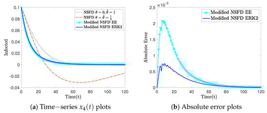
Figure 2. Test Case 2: Comparison of the modified NSFD EE and the modified NSFD ERK2 methods to other numerical methods, applied to Model (18), using step size $h=0.5$. For illustration purposes, only the infected population plots are shown.

Next, a comparison of the $l^{\infty }$ errors at the final time $T=120$ and convergence rates for the numerical solution obtained with various NSFD methods is presented in Table 2. The errors are calculated by using the numerical solution obtained on the finest grid as a benchmark. We observe from Table 2 that the solutions obtained using the modified NSFD EE and modified NSFD ERK2 methods again converge to the exact solution with rate 2, even for a nonlinear system, which also validates our theoretical results and the observations made in Figure 2.

Table 2. Test Case 2: Discrete $l^{\infty }$ error (top) and the rates of convergence (bottom) of the new modified NSFD EE and NSFD ERK2 methods for solving System (18).

h	Modified NSFD EE	Modified NSFD ERK2
$1.00\times {10}^0$	$1.73\times {10}^{-1}$	$5.32\times {10}^{-2}$
$5.00\times {10}^{-1}$	$1.61\times {10}^{-1}$	$3.13\times {10}^{-2}$
$2.50\times {10}^{-1}$	$1.36\times {10}^{-1}$	$1.22\times {10}^{-2}$
$1.25\times {10}^{-1}$	$9.09\times {10}^{-2}$	$3.56\times {10}^{-3}$
$6.25\times {10}^{-2}$	$4.02\times {10}^{-2}$	$9.34\times {10}^{-4}$
$3.12\times {10}^{-2}$	$1.26\times {10}^{-2}$	$2.39\times {10}^{-4}$
$1.56\times {10}^{-2}$	$3.41\times {10}^{-3}$	$6.14\times {10}^{-5}$
$7.81\times {10}^{-3}$	$8.96\times {10}^{-4}$	$1.61\times {10}^{-5}$
Rate	1.93	1.93

In Test Case 3, the predator–prey system with a Beddington–DeAngelis functional response in [32] is considered, with the notation $\overrightarrow{x}=(x_1,x_2)=(x,y)$:

$$\begin{array}{cc}\hfill {\displaystyle \frac{d{x}_1}{dt}}& =x_1-{\displaystyle \frac{A{x}_1{x}_2}{1+x_1+x_2}},\hfill \\ \hfill {\displaystyle \frac{d{x}_2}{dt}}& ={\displaystyle \frac{E{x}_1{x}_2}{1+x_1+x_2}}-D{x}_2,\hfill \end{array}$$

(19)

where $x_1$ and $x_2$ represent the prey and predator population sizes, respectively. Parameter values $A=6.0,D=5.0$, and $E=7.5$ are used in the numerical simulations. Stability analysis of System (19) reveals that there exist two equilibria [32]: $(0,0)$ and $\left({\displaystyle \frac{AD}{AE-E-AD}},{\displaystyle \frac{E}{AE-E-AD}}\right)=(4,1)$. The eigenvalues of the Jacobian matrix evaluated at $(0,0)$ are ${\lambda }_1=1$ and ${\lambda }_2=-5$, while the eigenvalues evaluated at $(4,1)$ are ${\lambda }_{3,4}=-{\displaystyle \frac{1}{12}}\pm i{\displaystyle \frac{\sqrt{119}}{12}}$, with $\left|{\lambda }_{3,4}\right|=0.9129$. Therefore, the coexistence equilibrium $(4,1)$ is globally asymptotically stable in the interior of the first quadrant, while $(0,0)$ is unstable.

The novel nonstandard denominator functions ${\phi }_i$ for the modified NSFD EE method are selected using Remark 1, as follows:

$${\phi }_i(h,\overrightarrow{x})=\left({\displaystyle \frac{1-exp(-\alpha h)}{\alpha }}\right)\left(1+tanh\left({\displaystyle \frac{\alpha -q_i(\overrightarrow{x})}{2}}h\right)\right),$$

for $i=1,2$, using

$$q_i(\overrightarrow{x})=-{\displaystyle \frac{\left(f_1(x_1,x_2)\frac{\partial f_i}{\partial x_1}+f_2(x_1,x_2)\frac{\partial f_i}{\partial x_2}\right)}{f_i(x_1,x_2)}},$$

where $f_1(x_1,x_2)=x_1-{\displaystyle \frac{A{x}_1{x}_2}{1+x_1+x_2}}$ and $f_2(x_1,x_2)={\displaystyle \frac{E{x}_1{x}_2}{1+x_1+x_2}}-D{x}_2$, and $\alpha =10.1>{max}_{\mathsf{\Omega }}{\displaystyle \frac{{\left|\lambda \right|}^2}{|Re(\lambda )|}}$. For the modified NSFD ERK2 method, the denominator function is chosen as $\phi (h)={\displaystyle \frac{tanh(qh)}{q}}$, with $q=5.1>{max}_{\mathsf{\Omega }}{\displaystyle \frac{{\left|\lambda \right|}^2}{2|Re(\lambda )|}}$, where $\mathsf{\Omega }={\bigcup }_{{\overrightarrow{x}}^{\ast }\in \mathsf{\Gamma }}\sigma (J({\overrightarrow{x}}^{\ast }))$, and $\mathsf{\Gamma }$ denotes the set of all hyperbolic equilibria ${\overrightarrow{x}}^{\ast }$ of System (1).

Figure 3 compares the modified NSFD EE method with the NSFD EE method for $h=0.02$. As can be seen in Figure 3a–c, there is a slight horizontal shift in both components of the numerical solution from the first-order NSFD EE method, while the numerical solution from the modified NSFD EE method converges much more accurately to the exact solution. In addition, absolute error plots, using the numerical solution on the finest grid as a benchmark, are presented in Figure 3d, where the new modified NSFD EE method clearly outperforms the NSFD EE method. A similar comparison of the numerical methods is presented in Figure 4, where the second-order modified NSFD ERK2 method outperforms the first-order NSFD ERK2 method for $h=0.05$.

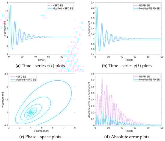
Figure 3. Test Case 3: Comparison of the modified NSFD EE method to the NSFD EE method, applied to Model (19), using $h=0.02$.

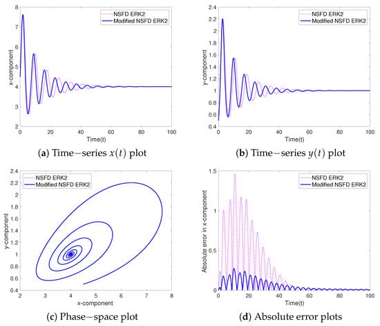
Figure 4. Test Case 3: Comparison of the modified NSFD ERK2 method to the NSFD ERK2 method, applied to Model (19), using $h=0.05$.

Next, we compare the execution time and the computational cost for the presented explicit second-order modified NSFD methods, modified NSFD explicit Euler and modified NSFD ERK2 methods, with the implicit Rosenbrock23 method or order 2 [42], the Magnus exponential integrator of order 2 [43], and the MATLAB^® built-in adaptive time-stepping solvers ode23s (based on the modified Rosenbrock formula of order 2), ode23, ode15s, and ode23t, with MATLAB’s default absolute tolerance of $1.00\times {10}^{-6}$ and relative tolerance of $1.00\times {10}^{-3}$ [44]. The simulations were performed using MATLAB R2022a on a MacBook Pro (13-inch Apple M1, Apple, Tokyo, Japan) with MacOS 14.4.1(23E224), 8 cores, and 16 Gb RAM; the results are displayed in Table 3. The execution time for each numerical method was calculated using MATLAB’s tic and toc functions to measure the elapsed time in seconds, while the computational cost coefficient was calculated as the ratio of the elapsed times for the numerical method to our corresponding explicit second-order modified NSFD method. There are alternative approaches of estimating the computational cost of the various methods used; nevertheless, our approach accurately reflects the relative performance of these methods. As can be seen in the table, our second-order modified NSFD ERK2 method is the most efficient integrator within this group of numerical methods, followed closely by our second-order modified NSFD explicit Euler method and MATLAB’s ode23 solver. This is in contrast with the other numerical integrators, particularly the Magnus exponential integrator and MATLAB’s ode23s solver, whose computational cost is the highest of all the methods considered. It is also important to note that the modified NSFD ERK2 method is more computationally efficient than the modified NSFD EE method. This is because the denominator function $\phi (h)$ in the modified NSFD ERK2 method is the same for all solution components and does not change over time (Theorem 2), whereas the denominator function ${\phi }_i(h,{\overrightarrow{x}}^k)$ in the modified NSFD EE method (Theorem 1) must be re-calculated for each solution component i and at every time step, making it the preferred modified NSFD method in Test Case 3.

Table 3. Comparison of the execution times, which was calculated using MATLAB’s tic and toc functions to measure the elapsed time in seconds, as well as the computational cost coefficients, which were calculated as the ratio of the elapsed times for the numerical method to our corresponding explicit second-order modified NSFD method, for each of the considered numerical methods.

		Modified NSFD EE	Modified NSFD ERK2	MATLAB® ode23s	MATLAB® ode23	MATLAB® ode15s	MATLAB® ode23t	Rosenbrock	Magnus
Execution time		$2.32\times {10}^{-2}$	$6.53\times {10}^{-3}$	$7.22\times {10}^{-2}$	$1.77\times {10}^{-2}$	$4.58\times {10}^{-2}$	$4.93\times {10}^{-2}$	$9.85\times {10}^{-2}$	$4.20\times {10}^{-1}$
Computational cost coefficient	Modified NSFD EE	1.00	0.28	3.11	0.76	1.97	2.13	4.24	18.1
	Modified NSFD ERK2	3.55	1.00	11.05	2.71	7.01	7.54	15.08	64.31

4. Conclusions

In this paper, two new classes of second-order modified nonstandard explicit Euler and explicit Runge–Kutta methods for multi-dimensional autonomous dynamical systems were presented and analyzed. The fundamental idea underlying the numerical methods’ development is the use of a novel modified nonstandard denominator function in the discretization of the derivative. In the case of the modified NSFD explicit Euler method, the denominator function is a product of two special functions. One of the functions satisfies the methods’ second-order accuracy property, while the other function satisfies the stability criteria of Theorem 1. For the modified nonstandard explicit Runge–Kutta method, a single denominator function suffices to satisfy both the elementary stability and second-order accuracy properties. Examples of denominator functions were presented that also serve as instructions for choosing generic ones. Next, the proposed modified nonstandard methods were applied to solve a biomass system, an MSEIR system, and a predator–prey system with a Beddington–DeAngelis functional response. The results obtained using the new numerical methods were compared to existing standard and nonstandard finite-difference methods, and it was observed that the new explicit modified NSFD methods demonstrate high accuracy and desirable stability properties, while still being computationally efficient and easy to implement.

References

- Mickens, R. Nonstandard Finite Difference Models of Differential Equations; World Scientific: Singapore, 1994. [Google Scholar]
- Dimitrov, D.; Kojouharov, H. Positive and elementary stable nonstandard numerical methods with applications to predator-prey models. J. Comput. Appl. Math. 2006, 189, 98–108. [Google Scholar] [CrossRef]
- Mickens, R.E. Numerical integration of population models satisfying conservation laws: NSFD methods. J. Biol. Dyn. 2007, 1, 427–436. [Google Scholar] [CrossRef] [PubMed]
- González-Parra, G.; Arenas, A.J.; Chen-Charpentier, B.M. Combination of nonstandard schemes and Richardson’s extrapolation to improve the numerical solution of population models. Math. Comput. Model. 2010, 52, 1030–1036. [Google Scholar] [CrossRef]
- Patidar, K.C.; Ramanantoanina, A. A non-standard finite difference scheme for a class of predator–prey systems with non-monotonic functional response. J. Differ. Equ. Appl. 2021, 27, 1310–1328. [Google Scholar] [CrossRef]
- Calatayud, J.; Jornet, M. An improvement of two nonstandard finite difference schemes for two population mathematical models. J. Differ. Equ. Appl. 2021, 27, 422–430. [Google Scholar] [CrossRef]
- Anguelov, R.; Lubuma, J.M.S. Forward invariant set preservation in discrete dynamical systems and numerical schemes for ODEs: Application in biosciences. Adv. Contin. Discret. Model. 2023, 2023. [Google Scholar] [CrossRef]
- Alalhareth, F.K.; Mendez, A.C.; Kojouharov, H.V. A simple model of nutrient recycling and dormancy in a chemostat: Mathematical analysis and a second-order nonstandard finite difference method. Commun. Nonlinear Sci. Numer. Simul. 2024, 132, 107940. [Google Scholar] [CrossRef]
- Arenas, A.J.; Moraño, J.A.; Cortés, J.C. Non-standard numerical method for a mathematical model of RSV epidemiological transmission. Comput. Math. Appl. 2008, 56, 670–678. [Google Scholar] [CrossRef]
- Anguelov, R.; Dumont, Y.; Lubuma, J.S.; Shillor, M. Comparison of Some Standard and Nonstandard Numerical Methods for the MSEIR Epidemiological Model. AIP Conf. Proc. 2009, 1168, 1209–1212. [Google Scholar]
- Arenas, A.J.; González-Parra, G.; Chen-Charpentier, B.M. A nonstandard numerical scheme of predictor–corrector type for epidemic models. Comput. Math. Appl. 2010, 59, 3740–3749. [Google Scholar] [CrossRef]
- Garba, S.; Gumel, A.; Lubuma, J.S. Dynamically-consistent non-standard finite difference method for an epidemic model. Math. Comput. Model. 2011, 53, 131–150. [Google Scholar] [CrossRef]
- Obaid, H.A.; Ouifki, R.; Patidar, K.C. An unconditionally stable nonstandard finite difference method applied to a mathematical model of HIV infection. Int. J. Appl. Math. Comput. Sci. 2013, 23, 357–372. [Google Scholar] [CrossRef]
- Anguelov, R.; Dumont, Y.; Lubuma, J.; Shillor, M. Dynamically consistent nonstandard finite difference schemes for epidemiological models. J. Comput. Appl. Math. 2014, 255, 161–182. [Google Scholar] [CrossRef]
- Berge, T.; Lubuma, J.S.; Moremedi, G.; Morris, N.; Kondera-Shava, R. A simple mathematical model for Ebola in Africa. J. Biol. Dyn. 2017, 11, 42–74. [Google Scholar] [CrossRef]
- Obaid, H.A.; Ouifki, R.; Patidar, K.C. A nonstandard finite difference method for solving a mathematical model of HIV-TB co-infection. J. Differ. Equ. Appl. 2017, 23, 1105–1132. [Google Scholar] [CrossRef]
- Anguelov, R.; Dukuza, K.; Lubuma, J.M.S. Backward bifurcation analysis for two continuous and discrete epidemiological models. Math. Methods Appl. Sci. 2018, 41, 8784–8798. [Google Scholar] [CrossRef]
- Anguelov, R.; Berge, T.; Chapwanya, M.; Djoko, J.; Kama, P.; Lubuma, J.M.S.; Terefe, Y. Nonstandard finite difference method revisited and application to the Ebola virus disease transmission dynamics. J. Differ. Equ. Appl. 2020, 26, 818–854. [Google Scholar] [CrossRef]
- Vaz, S.; Torres, D.F.M. A dynamically-consistent nonstandard finite difference scheme for the SICA model. Math. Biosci. Eng. 2021, 18, 4552–4571. [Google Scholar] [CrossRef]
- Adamu, E.M.; Patidar, K.C.; Ramanantoanina, A. An unconditionally stable nonstandard finite difference method to solve a mathematical model describing Visceral Leishmaniasis. Math. Comput. Simul. 2021, 187, 171–190. [Google Scholar] [CrossRef]
- Chapwanya, M.; Lubuma, J.; Terefe, Y.; Tsanou, B. Analysis of War and Conflict Effect on the Transmission Dynamics of the Tenth Ebola Outbreak in the Democratic Republic of Congo. Bull. Math. Biol. 2022, 84, 136. [Google Scholar] [CrossRef]
- Ouemba Tassé, A.J.; Kubalasa, V.B.; Tsanou, B.; Jean, M.-S.L. Nonstandard finite difference schemes for some epidemic optimal control problems. Math. Comput. Simul. 2024, 228, 1–22. [Google Scholar] [CrossRef]
- Bruggeman, J.; Burchard, H.; Kooi, B.W.; Sommeijer, B. A second-order, unconditionally positive, mass-conserving integration scheme for biochemical systems. Appl. Numer. Math. 2007, 57, 36–58. [Google Scholar] [CrossRef]
- Benz, J.; Meister, A.; Zardo, P. A conservative, positivity preserving scheme for advection-diffusion-reaction equations in biochemical applications. In Hyperbolic Problems: Theory, Numerics and Applications, Proceedings of the Twelfth International Conference on Hyperbolic Problems, Center for Scientific Computation and Mathematical Modeling, University of Maryland, College Park, MD, USA, 9–13 June 2008; Tadmor, E., Liu, J.G., Tzavaras, A., Eds.; American Mathematical Society: Providence, RI, USA, 2009; Volume 67, pp. 399–408. [Google Scholar]
- Burchard, H.; Deleersnijder, E.; Meister, A. A high-order conservative Patankar-type discretisation for stiff systems of production–destruction equations. Appl. Numer. Math. 2003, 47, 1–30. [Google Scholar] [CrossRef]
- Wood, D.; Dimitrov, D.; Kojouharov, H. A nonstandard finite difference method for n-dimensional productive-destructive systems. J. Differ. Equ. Appl. 2015, 21, 240–254. [Google Scholar] [CrossRef]
- Patidar, K.C. On the use of nonstandard finite difference methods. J. Differ. Equ. Appl. 2005, 11, 735–758. [Google Scholar] [CrossRef]
- Patidar, K.C. Nonstandard finite difference methods: Recent trends and further developments. J. Differ. Equ. Appl. 2016, 22, 817–849. [Google Scholar] [CrossRef]
- Mickens, R.E. Nonstandard Finite Difference Schemes; World Scientific: Singapore, 2020. [Google Scholar]
- Anguelov, R.; Lubuma, J. Contributions to the mathematics of the nonstandard finite difference method and applications. Numer. Methods Partial. Differ. Equ. 2001, 17, 518–543. [Google Scholar] [CrossRef]
- Lubuma, J.M.S.; Roux, A. An Improved Theta-method for Systems of Ordinary Differential Equations. J. Differ. Equ. Appl. 2003, 9, 1023–1035. [Google Scholar] [CrossRef]
- Dimitrov, D.; Kojouharov, H. Nonstandard finite-difference schemes for general two-dimensional autonomous dynamical systems. Appl. Math. Lett. 2005, 18, 769–774. [Google Scholar] [CrossRef]
- Dang, Q.A.; Hoang, M.T. Positive and elementary stable explicit nonstandard Runge-Kutta methods for a class of autonomous dynamical systems. Int. J. Comput. Math. 2020, 97, 2036–2054. [Google Scholar] [CrossRef]
- Gupta, M.; Slezak, J.; Alalhareth, F.; Roy, S.; Kojouharov, H.V. Second-order Modified Nonstandard Explicit Runge-Kutta And Theta Methods for One-dimensional Autonomous Differential Equations. Appl. Appl. Math. Int. J. (AAM) 2021, 16, 788–803. [Google Scholar]
- Hoang, M.T. A novel second-order nonstandard finite difference method for solving one-dimensional autonomous dynamical systems. Commun. Nonlinear Sci. Numer. Simul. 2022, 114, 106654. [Google Scholar] [CrossRef]
- Roeger, L.I.W. Nonstandard finite-difference schemes for the Lotka–Volterra systems: Generalization of Mickens’s method. J. Differ. Equ. Appl. 2006, 12, 937–948. [Google Scholar] [CrossRef]
- Izgin, T.; Kopecz, S.; Meister, A. On the stability of unconditionally positive and linear invariants preserving time integration schemes. SIAM J. Numer. Anal. 2022, 60, 3029–3051. [Google Scholar] [CrossRef]
- Izgin, T.; Kopecz, S.; Meister, A. On Lyapunov stability of positive and conservative time integrators and application to second order modified Patankar–Runge–Kutta schemes. ESAIM Math. Model. Numer. Anal. 2022, 56, 1053–1080. [Google Scholar] [CrossRef]
- Wood, D.T.; Kojouharov, H.V.; Dimitrov, D.T. Universal approaches to approximate biological systems with nonstandard finite difference methods. Math. Comput. Simul. 2017, 133, 337–350. [Google Scholar] [CrossRef]
- Songolo, M.E.; Bidégaray-Fesquet, B. Extending nonstandard finite difference scheme rules to systems of nonlinear ODEs with constant coefficients. J. Differ. Equ. Appl. 2024, 30, 577–602. [Google Scholar] [CrossRef]
- Quarteroni, A.; Sacco, R.; Saleri, F. Numerical Mathematics; Springer: Berlin/Heidelberg, Germany, 2007; 657p. [Google Scholar]
- Dear, J.; Shi, Z.; Lin, J. An efficient numerical integration system for stiff unified constitutive equations for metal forming applications. IOP Conf. Ser. Mater. Sci. Eng. 2022, 1270, 012008. [Google Scholar] [CrossRef]
- Hajiketabi, M.; Casas, F. Numerical integrators based on the Magnus expansion for nonlinear dynamical systems. Appl. Math. Comput. 2020, 369, 124844. [Google Scholar] [CrossRef]
- Shampine, L.F.; Reichelt, M.W. The MATLAB ODE Suite. SIAM J. Sci. Comput. 1997, 18, 1–22. [Google Scholar] [CrossRef]
Disclaimer/Publisher’s Note: The statements, opinions and data contained in all publications are solely those of the individual author(s) and contributor(s) and not of MDPI and/or the editor(s). MDPI and/or the editor(s) disclaim responsibility for any injury to people or property resulting from any ideas, methods, instructions or products referred to in the content. |
© 2024 by the authors. Licensee MDPI, Basel, Switzerland. This article is an open access article distributed under the terms and conditions of the Creative Commons Attribution (CC BY) license (https://creativecommons.org/licenses/by/4.0/).